A Model of Competing Gangs in Networks

Abstract

Two groups produce a network good perceived by a third party, such as a police or military institution, as a ‘public bad’, referred to as ‘crime’ for simplicity. These two groups, considered mafias, are assumed to be antagonists, whether they are enemies or competitors in the same market, causing harm to each other’s activities. This paper provides guidelines for the policymaker, typically the police, seeking to minimize overall crime levels by internalizing these negative externalities. One specific question is investigated: the allocation of resources for the police. In general, we recommend a balanced crackdown on both antagonists, but an imbalance in group sizes may lead the police to focus on the more criminal group.

1. Introduction

The impact of networks on agents’ decisions has been a topic of ongoing interest across various fields, ranging from sociology to economics and game theory. The pioneering work by Ballester et al. [1], presenting a model incorporating positive and negative externalities, has sparked considerable attention regarding the role of network influences in amplifying or inhibiting agents’ efforts. Along with the properties of the utility functions chosen by the authors, which make the model particularly relevant for crime settings, this combination of externalities of both types invites us to consider groups of criminals. Other noteworthy contributions, including perspectives on delinquent behavior or social norms, are found in works by Calvó-Armengol and Zenou [2], Cao et al. [3], Calvó-Armengol et al. [4], Ballester et al. [5], Ushchev and Zenou [6]. The current paper explores a specific issue related to the coexistence of positive and negative externalities within a network, specifically when society is polarized. We apply the classical structure of Harary [7] to capture society’s separation into two rival mafias, with externality being positive within groups and negative across groups.

1.1. Motivation

The initial model of Ballester et al. [1] allowed for perfectly heterogeneous network influences. In the context of a balanced network (the directed graphs version of Harary [7]), this heterogeneity collapses into two groups, within which externalities are positive, and across which externalities are negative.

In the context of delinquent networks, the issue indeed revolves around competition between gangs. While both gangs contribute to crime within their groups, they may also engage in inter-gang conflicts, such as competing for the control of the drug market and impeding on each other’s activities, thereby diminishing their overall criminal activities. From society’s perspective, only aggregate crime level matters, and one may wonder how civil society, as proxied by the police, could instrumentalize the conflict, possibly by brokering deals with gangs for social peace.

Throughout the paper, we use the term ‘crime’ for simplicity and because the setting is relevant enough to deserve particular interest. However, our results could accommodate a broader range of similar strategic interactions: a military opposition between two republics within a federation, cyberattacks between rival hackers, or any strategic interaction that hampers the rivals’ activities. We may consider the collaboration between two countries in military, scientific, energy, or diplomatic ventures perceived as a threat to a third country. This third country might contemplate opposing both countries to thwart their activities—whether on a diplomatic or military basis, adopting a ‘realpolitik’ stance, reaching an agreement with one to oppose the other, or sparking a conflict against only one.

Returning to criminal activity, and by investigating the allocation of resources in the government’s fight against gangs, our goal is to elucidate the contradicting effects at play to reach a society’s crime level as low as possible. The particular setting of a three-player game—two mafias and the police—establishes the context at a high level of aggregation and allows us to address, in place of the police, the problem of internalizing negative externalities, thereby reducing the overall level of crime. This question will be examined from the perspective of resource allocations, with the police choosing which group to direct its action against.

As compared with Ballester et al. [1], whose main contribution is to identify and remove the ‘key player’, i.e., the one with the highest inter-centrality (which is not necessarily the one exerting the highest effort), our approach differs and operates at a lower level of granularity. More specifically, in Ballester et al. [1], there is no cost analysis for the police intervention, even though targeting the key player may prove costly since, for example, reconstituting a delinquent network is a real possibility, especially in prisons. Our approach aggregates the activities of agents to encompass a group decision-making aspect and proposing guidelines based on the group’s autarkic activities for a third party with the power to impact the game. When gangs are of equal size, we demonstrate that the optimal strategy for the third party is to equally share the resources invested in cracking down on crime against the two groups. However, under the hypothesis of our model, we also show that these results are sensitive to the inequality in the activity/size of the groups and that unequal sizes may turn into exclusive attention against the group of the highest activity, referred to as “the strongest group” (or the “most criminal”), as measured by its autarkic activity (the strongest group is therefore not necessarily the one with the highest cardinality).

Finding the most adequate intervention will surely depend on the type of network and the groups under investigation, but our aggregate approach provides more flexibility by favoring a more diffuse intervention. Even though the removal of the key player could be extended to key groups, as done in Temurshoev [8], and even when computational issues can be successfully addressed in practice, mistakes could have severe implications in terms of resource utilization. Also, bounded information and rationality issues exert severe limitations on the key player approach. On the contrary, since our analysis only needs to know the aggregate crime levels of gangs, it is situated at a coarser granularity: in the presence of limited information about the exact architecture of the network, the police only needs to know the aggregate level of crime, not the exact interactions of criminals.

1.2. Related Work

Generally speaking, the broad notion of network influence designates structured interactions. In some circumstances, the word ‘influence’ may refer to information considerations, as seen in the context of rumors [9], votes [10,11,12,13], diffusion [14,15,16], opinion formation [17,18,19,20,21,22,23], status [24], homophily [25], learning [26], cultural traits [27], epidemiological tensions [28], collective games [29], or information extraction [30,31,32], not forgetting the anthropological studies on mimikry behavior by Girard [33,34,35,36], where imitation departs from rational decisions but now emerges either from the attribution of prestige perceived by the imitator in a model or from contagion in a society under crisis searching for a scapegoat.

In Ballester et al. [1], where effort equates with crime and externalities with influences, positive and negative influences receive different interpretations. A positive influence exacerbates crime, while a negative one, a notion related to but distinct from ‘anti-conformism’ [37,38,39] or anti-coordination [40,41,42], plays down on agents’ level of action. We can think of a ‘first-mover advantage’ over meeting a demand, e.g., in a drug market. This flexible model, which we will rely on to investigate the particular problem of competing gangs, encapsulates various situations under standard assumptions.

The Ballester et al. [1] model belongs to the family of models with continuous actions/opinions and static decisions: there is no ‘repeated game’ dimension, as we could find, e.g., in opinion formation models [17,22,43,44,45], mainly focusing their interest on opinion reversal and diffusion [25,46,47], including in development economics [16]. Its main technical difficulty is the nonnegativity of actions, raising the delicate question of the interiority of equilibrium and the actual network of active players (see, for example, Bramoullé and Kranton [48] for a standard model on a similar framework).

Among the other workhorse models of this literature, the key paper of Bramoullé et al. [49] also investigates public goods in networks in the vein of Ballester et al. [1] and Ballester and Zenou [50], where the network good is actually a kind of ‘public bad’. The problem had already been investigated in the context of groups by Buchholz et al. [51]. In an economy, one group perceives the action as good and the other as bad. Other frameworks have also been proposed, e.g., Cabrales et al. [52], encompassing network formation and the productive side in a single spillover model.

Though the key player does not play a role in our model, the aggregation of individual activities remains dependent on the network’s topology, and this topology is typically a sociological dimension of the problem. Therefore, we have to mention the theory of social power, where the position in the network is central; see, for example, Friedkin [53], de Swart and Rusinowska [54], van den Brink and Steffen [55]. In contrast with models like that of Acemoglu et al. [56], where leaders are specifically designed, leadership may also emerge from centrality, which ties the notion of power to topological considerations [53,57,58,59,60]. In the literature on social and economic networks, the role of an agent’s position in the network in the outcome of a game is a standard field of investigation; we refer to Jackson [61], Bramoullé et al. [62] for two authoritative reviews of theoretical models on social and economic networks.

1.3. Organization of the Paper

The paper is structured as follows. The outlines of the Ballester et al. [1] model and the specific setting we will be studying are exposed in Section 2. Policy recommendations for the police are discussed in Section 3. Section 4 concludes with the limitations of our model and some perspectives.

2. The Model

Our model adapts Ballester et al. [1,5] in a specific setting involving two rival groups. We consider crime networks as a practical application of the model, given that the properties of the utility functions align well with the impact of agents’ actions (not only utilities) based on whether these actions originate from allies or enemies, as we will see below. A notable departure from the concerns addressed by Ballester et al. [1] is that we focus on examining aggregate levels within groups rather than targeting a key player. In particular, the significance of the network’s architecture is only relevant in terms of its consequences on an aggregate scale.

We denote by N the set of n agents (criminals) in a network. Agents are located on an undirected and unweighted network described by the adjacency matrix G. If agent $j\ne i$ is a neighbor of i then $g_{ij}=1$, otherwise $g_{ij}=0$. The set of neighbors of i is denoted by ${\mathcal{N}}_i$, i.e., ${\mathcal{N}}_i:=\{j\mid g_{ij}\ne 0\}$. Each agent i exerts a level of effort $x_i\ge 0$ and obtains utility $u_i(x_i,{\mathbf{x}}_{-i})$, where ${\mathbf{x}}_{-i}$ is the vector of efforts exerted by other agents (we use bold lowercase letters for vectors).

The utility functions are taken quadratic:

$$u_i(x_i,{\mathbf{x}}_{-i})=x_i-\frac{1}{2}{x}_i^2+\sum _{j\in {\mathcal{N}}_i}{\beta }_{ij}{x}_i{x}_j,$$

(1)

where ${\beta }_{ij}$ denotes the nature and intensity of the externality between agents i and j.

In interpretation, when ${\beta }_{ij}>0$ efforts are strategic complements and when ${\beta }_{ij}<0$ efforts are strategic substitutes. This observation, specific to the family of bilinear utility functions, is the one that justifies their use to model delinquent networks. Individual effort is then identified with crime. A positive network influence ${\beta }_{ij}>0$ can be thought of as an incentive to commit crime (commonly known as ‘bad company’) or, e.g., as an exacerbation of violence between criminals. On the contrary, ${\beta }_{ij}<0$ can be thought of as the control of a drug market, where some criminals’ actions impede others’ actions.

An agent i seeks to maximize their payoffs and has a best-response function:

$$x_i=f_i\left({\mathbf{x}}_{-i}\right)\stackrel{\mathrm{def}}{=}max\left(0,1+\sum _{j\in {\mathcal{N}}_i}{\beta }_{ij}{x}_j\right).$$

(2)

At a Nash equilibrium ${\mathbf{x}}^{\ast }=(x_1^{\ast },\dots ,x_n^{\ast })$ of the game, each agent’s action is a best-response to their neighbors’ actions, that is, $x_i^{\ast }=f_i\left({\mathbf{x}}_{-i}^{\ast }\right)$ for each agent $i\in N$.

We now apply the Ballester et al. [1] model to our two competing groups model. The society is partitioned into two groups, A and B, of sizes $n_A$ and $n_B$. To simplify the computations:

• We restrict our analysis to two concurrent groups, i.e., that exert negative externalities on each other (communitarian model with two groups).
• All externalities are of the same intensity within group $\delta \ge 0$ and inter-group $-\mu \le 0$.
• We consider the ’full inter-connection case’, where any two agents of different groups are linked. One interpretation of the full interconnection case is that inter-group confrontations are uniform in the sense that the aggregate crime production of the opposite group hurts each agent. Another interpretation is probabilistic: $\mu$ represents the probability of facing each agent of the opposite group.

From the assumptions above (in particular, since for $i\in A$, $B\cap {\mathcal{N}}_i=B$, by the full inter-connection case), we can rewrite (1) as follows. If $i\in A$, then:

$$u_i(x_i,{\mathbf{x}}_{-i})=\left[x_i-\frac{1}{2}{x}_i^2+\delta x_i\sum _{j\in A\cap {\mathcal{N}}_i}{x}_j-\mu x_i\sum _{j\in B}{x}_j\right].$$

(3)

Similarly, if $i\in B$, then:

$$u_i(x_i,{\mathbf{x}}_{-i})=\left[x_i-\frac{1}{2}{x}_i^2+\delta x_i\sum _{j\in B\cap {\mathcal{N}}_i}{x}_j-\mu x_i\sum _{j\in A}{x}_j\right].$$

(4)

Let ${\mathbf{\Gamma }}_{\left[AA\right]}=\mathbf{I}-\delta {\mathbf{G}}_A$ where ${\mathbf{G}}_A$ denotes the adjacency matrix of the network of interactions within group A and lets ${\mathbf{\Gamma }}_{\left[BB\right]}=\mathbf{I}-\delta {\mathbf{G}}_B$ where ${\mathbf{G}}_B$ denotes the adjacency matrix of the network of interactions within group B. Let us write

$$\mathbf{\Gamma }=\left[\begin{array}{cc}{\mathbf{\Gamma }}_{\left[AA\right]}& {\mathbf{\Gamma }}_{\left[AB\right]}\\ {\mathbf{\Gamma }}_{\left[BA\right]}& {\mathbf{\Gamma }}_{\left[BB\right]}\end{array}\right],$$

where ${\mathbf{\Gamma }}_{\left[AB\right]}$ and ${\mathbf{\Gamma }}_{\left[BA\right]}$ denote the links connecting A to B and B to A. Since we assume the ‘full inter-connection case’, it holds that all the entries of ${\mathbf{\Gamma }}_{\left[AB\right]}$ and ${\mathbf{\Gamma }}_{\left[BA\right]}$ are $\mu$. In our model, a Nash equilibrium is interior when all agents in the network exert a strictly positive level of effort (crime).

Property 1.

When it exists, the interior Nash equilibrium ${\mathbf{x}}^{\ast }$ verifies:

$$\mathbf{\Gamma }{\mathbf{x}}^{\ast }=\mathbf{1},$$

where $\mathbf{1}$ is the vector whose all coordinates are 1.

Proof. 

Indeed, at an interior Nash equilibrium ${\mathbf{x}}^{\ast }$, it follows from the best response functions that for an agent $i\in A$ it holds that:

$$x_i^{\ast }=1+\delta \sum _{j\in A\cap {\mathcal{N}}_i}{x}_j^{\ast }-\mu \sum _{j\in B}{x^{\ast }}_j.$$

(5)

and for an agent $i\in B$, it holds that:

$$x_i^{\ast }=1+\delta \sum _{j\in B\cap {\mathcal{N}}_i}{x}_j^{\ast }-\mu \sum _{j\in A}{x}_j^{\ast }.$$

(6)

By re-arranging (5) and (6) we obtain

$$\mathbf{\Gamma }{\mathbf{x}}^{\ast }=\mathbf{1}.$$

□

Let us define ${\mathbf{x}}_A:={\mathbf{\Gamma }}_{\left[AA\right]}^{-1}\mathbf{1}$ and ${\mathbf{x}}_B:={\mathbf{\Gamma }}_{\left[BB\right]}^{-1}\mathbf{1}$. We also consider $x_A:={\mathbf{1}}^T·{\mathbf{x}}_A$ and $x_B:={\mathbf{1}}^T·{\mathbf{x}}_B$, which represent the autarkic crime levels in groups A and B, respectively (note that the expression ${\mathbf{1}}^T·\mathbf{y}$ denotes the sum of the entries in the vector $\mathbf{y}$). The next result provides a closed-form expression of the production of crime ${\mathbf{x}}^{\ast }$, as a function of the autarkic productions of crime ${\mathbf{x}}_A$ and ${\mathbf{x}}_B$, namely, the crime levels produced if each of the two groups was alone, or if they were not impeding on each other’s actions ($\mu =0$). In the sequel, we will also write $x^{\ast }:={\mathbf{1}}^T·{\mathbf{x}}^{\ast }$ the total quantity of crime, or (total) crime level, defined as the sum of all individual contributions (both groups together). $x^{\ast }$ is arguably the only relevant crime index from the police perspective, aiming to achieve the highest possible level of societal safety.

Theorem 1 is based on two assumptions: first, that negative externalities are not excessively high, and second, the positive-definiteness of the matrix of interactions $\mathbf{\Gamma }$, that ensures a unique Nash equilibrium.

Theorem 1.

Assume that $\mu \le \frac{1}{\max (x_A,x_B)}$ and Γ is positive-definite. Then, there exists a unique Nash equilibrium, which is interior, and which has an expression as follows:

$${\mathbf{x}}^{\ast }=\frac{1}{1-{\mu }^2{x}_A{x}_B}·\left(\begin{array}{c}(1-\mu x_B)·{\mathbf{x}}_A\\ (1-\mu x_A)·{\mathbf{x}}_B\end{array}\right)=:\left(\begin{array}{c}{\mathbf{x}}_A^{\ast }\\ {\mathbf{x}}_B^{\ast }\end{array}\right).$$

Proof. 

The proof of Theorem 1, together with all the subsequent proofs, appears in the Appendix A. □

We will now provide a sufficient condition on the interaction network that ensures that $\mathbf{\Gamma }$ is positive definite, as stipulated in Theorem 1. Given a matrix $\mathbf{G}$, let ${\lambda }_{\max }\left(\mathbf{G}\right)$ denote its largest eigenvalue and ${\lambda }_{\min }\left(\mathbf{G}\right)$ denote its lowest eigenvalue.

Proposition 1.

Assume that $1-\delta \max ({\lambda }_{\max }\left({\mathbf{G}}_A\right),{\lambda }_{\max }\left({\mathbf{G}}_B\right))-\mu \sqrt{n_A{n}_B}>0.$ Then, $\mathbf{\Gamma }$ is positive definite.

It follows from Theorem 1 that when, for example, $x_A<x_B$, Group A (the group with the smaller autarkic crime level) is impacted by a higher reduction factor than Group B.

We are now in a position to express, in Proposition 2, the crime level $x^{\ast }$ as a function of each group’s autarkic activities, along with a few of its properties.

Proposition 2.

Under the assumptions and with the notations of Theorem 1:

(i) 

The crime level $x^{\ast }$ is:

$$x^{\ast }=\frac{(1-\mu x_B)x_A+(1-\mu x_A)x_B}{1-{\mu }^2{x}_A{x}_B}=\frac{x_A+x_B-\frac{2}{\mu }}{1-{\mu }^2{x}_A{x}_B}+\frac{2}{\mu }.$$

(For $\mu \ne 0$ in the second equality.)

(ii) 

$x^{\ast }\le x_A+x_B$.

(iii) 

Suppose that $x_A+x_B$ is fixed. Then, $x^{\ast }-(x_A+x_B)$ attains its maximum when $x_A=x_B$.

Proposition 2 shows how much the links between the two groups reduces the total crime level. We also proved that, given a fixed sum of the autarkic levels of crime, the maximum total crime reduction is achieved when the two groups have identical autarkic crime levels (Proposition 2iii).

Example 1.

Let us investigate the case of regular networks within each group to push the computations forward. We assume that internal networks for the groups are regular of degrees $r_A$ and $r_B$, respectively. Then, ${\mathbf{x}}_A$ and ${\mathbf{x}}_B$ can be expressed in terms of the degree of the regular network and the discount factor (see Allouch [63], Proposition 7): ${\mathbf{x}}_A=\frac{1}{1-\delta r_A}\mathbf{1}$, ${\mathbf{x}}_B=\frac{1}{1-\delta r_B}\mathbf{1}$, and therefore $x_A=\frac{n_A}{1-\delta r_A}$ and $x_B=\frac{n_B}{1-\delta r_B}$. We obtain:

$$x^{\ast }=\frac{(1-\delta r_A-\mu n_A)n_B+(1-\delta r_B-\mu n_B)n_A}{(1-\delta r_A)(1-\delta r_B)-{\mu }^2{n}_A{n}_B}.$$

If, for example, we have $n_A=n_B=4$ and $r_A=r_B=2$, then we obtain:

$$x_A=x_B=\frac{4}{1-2\delta }\mathit{and}{x}^{\ast }=\frac{8}{1-2\delta +4\mu }.$$

(7)

From (7), we see that policies decreasing the emulation factor δ (we can think, for example, of an “education approach” aimed at increasing the opportunity cost of engaging in terrorist activities1) unambiguously decreases the crime level. However, very interestingly, if the police had a choice between decreasing the emulation factor δ by ϵ or increasing the inter-group fight intensity μ by ϵ, the latter policy will outperform the former policy.

Let us end this example with one question: What is the effect of degrees of unbalance on the aggregate level of crime? Let us redo the computations with $n_A=n_B=n$ but with potentially different degrees $r_A$ and $r_B$, such that $r_A+r_B=K$, where K is a constant (also even):

$$x^{\ast }=\frac{2n-\delta K-2\mu n^2}{(1-\delta r_A)(1-\delta K+\delta r_A)-{\mu }^2{n}^2}.$$

$$\frac{d{x}^{\ast }}{d{r}_A}=\frac{-(2n-\delta K-2\mu n^2)({\delta }^{2}K-2{\delta }^2{r}_A)}{{((1-\delta r_A)(1-\delta K+\delta r_A)-{\mu }^2{n}^2)}^2},$$

which is null if and only if $r_A=\frac{K}{2}$, that is, $r_A=r_B$. This extremum represents a minimum. The total quantity of crime is minimized when groups possess identical internal degrees. In interpretation, the equality of internal degrees results in similar crime levels for the two groups, exacerbating losses on both sides and ultimately leading to a reduced total quantity of crime.

Scenario 1.

Given our focus on the internalization of negative externalities, there is a compelling case for concern regarding the unification of the groups. It is crucial to assess whether these groups may share common interests and, specifically, to gauge the strength of the threat that they might abruptly merge into a single mafia. The more similar the groups, the more pronounced the threat becomes. From the perspective of law enforcement, what would be the consequences if, instead of opposing each other, the two groups were to unite? (In a sense, what is the incentive for ‘making mischief’?) We calculate the total quantity of crime by replacing μ with $-\mu$. Consequently, the total quantity of crime in the unified case is as follows:

$$y^{\ast }=\frac{(1+\mu x_B)x_A+(1+\mu x_A)x_B}{1-{\mu }^2{x}_A{x}_B}=\frac{x_A+x_B+\frac{2}{\mu }}{1-{\mu }^2{x}_A{x}_B}-\frac{2}{\mu }.$$

As a consequence, the premium of causing mischief is given by:

$$y^{\ast }-x^{\ast }=\frac{4\mu x_A{x}_B}{1-{\mu }^2{x}_A{x}_B}.$$

It is noteworthy that, at a given total autarkic production of crime (for a given $x_A+x_B$), the more equal the groups are ($x_A\approx x_B$), the higher the fighting premium is from the perspective of the police. This observation aligns with the findings of Example 1.

3. Consequence for the Police: Focusing or Splitting the Resources?

In this section, our goal is to answer the question: Where should the police allocate its resources to minimize the quantity of crime?

We will explore two extreme cases. In Scenario 2, the effect on crime in both groups is assumed to be proportional to the effort of the police. This assumption reflects a situation where the police conducts random controls against drugs, implements reinforced patrols, or takes any action characterized by the absence of scale. In Scenario 3, the effect depends on the mafia size. This multiplicative assumption involves attributing an effect on crime proportional to the group’s size being fought against. This aims to represent a situation where there are ‘economies of scale’ concerning the effort of the police, such as in scenarios involving infiltration or cybersecurity measures against a specific threat type, where the difficulty of dismantling a network does not depend much on its size. In reality, the impact of spending is likely to be a combination of these two extreme scenarios.

In both scenarios, the police is assumed to have a budget that it divides into two parts. Specifically, an amount $ϵ\in [0,1]$ is allocated to combat Group A, and an amount $1-ϵ\in [0,1]$ is allocated to combat Group B. It is essential to note that the quantitative effect, i.e., how efficient this crackdown on crime actually is, is not considered at a higher level of policy-making. No parliament responsible for budget approval contemplates the expected impact of cracking down on crime, which would need to be balanced with other types of spending for the public sector. Nevertheless, we present, in our simulations, the actual impact on crime levels of an optimal policy.

Scenario 2

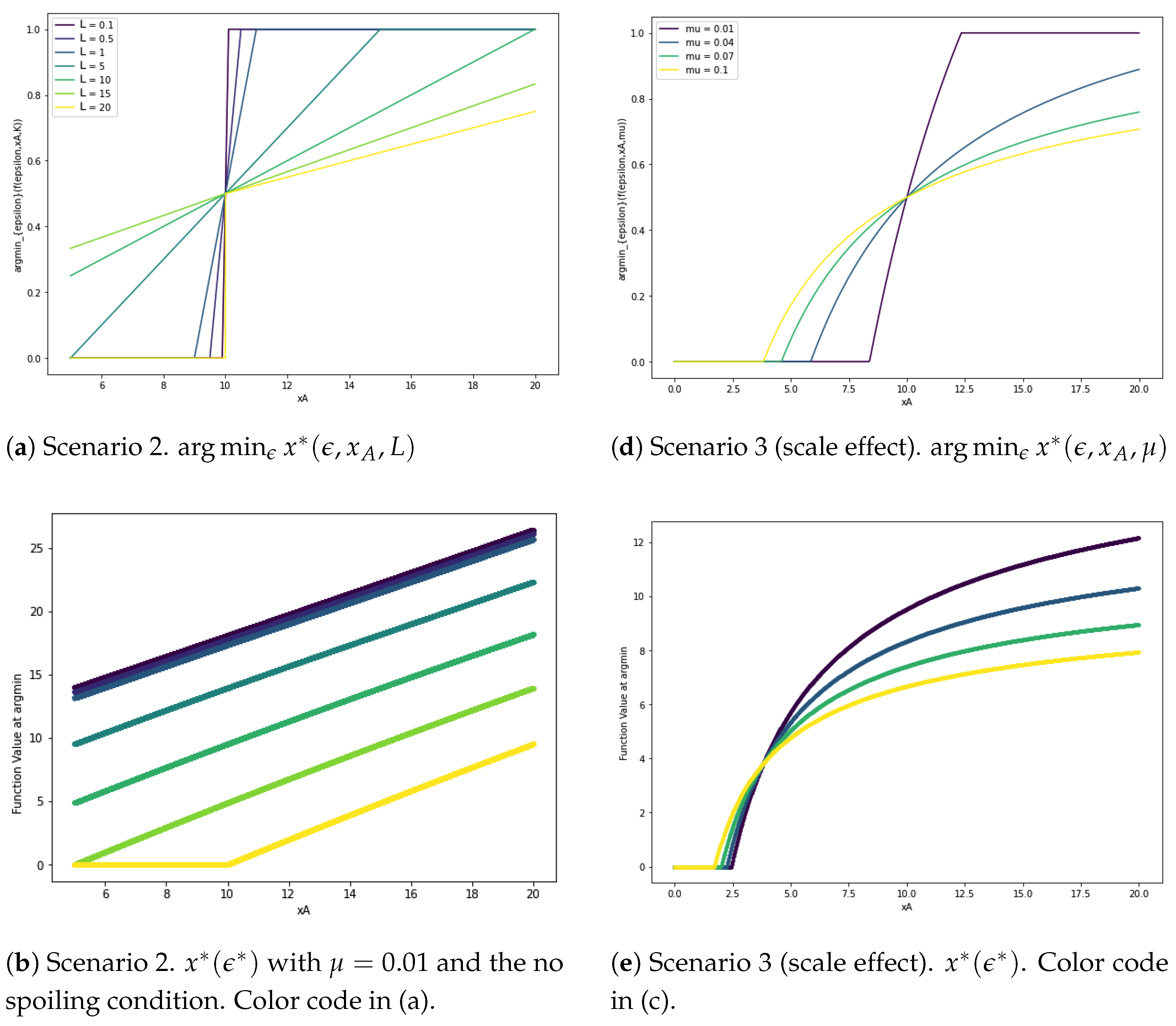
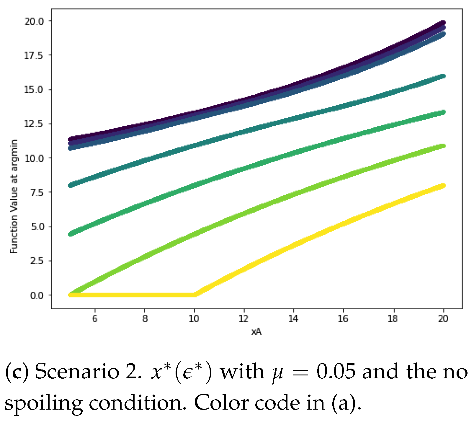
(An impact on crime with proportional effects). As a first extreme assumption, the present scenario assumes the decrease in crime to be directly proportional to the resources, meaning that spending ϵ results in a decrease in crime of $L·ϵ$, for some constant L. For $x_A\ne x_B$, let us first treat the case $\mu =0$. In the absence of police, the crime level is simply the sum of autarkic levels: $x^{\ast }=x_A+x_B$. Under police action, we have $x^{\ast }=(x_A-Lϵ)+(x_B-L(1-ϵ))=x_A+x_B-L$, which does not depend on ϵ: all repartitions of resources are equivalent for the police in terms of decision making. However, the crime level depends linearly on L; as we will see in Figure 1b,c, the effect is more sophisticated when $\mu \ne 0$, which is the case we examine now. Applying the first equality of Proposition 2, if $x^{\ast }$ is interior, then:

$$x^{\ast }=\frac{(1-\mu (x_B-L(1-ϵ)))(x_A-Lϵ)+(1-\mu (x_A-Lϵ))(x_B-L(1-ϵ))}{1-{\mu }^2(x_A-Lϵ)(x_B-L(1-ϵ))}.$$

The derivative with respect to ϵ of the total amount of crime is:

$$\frac{d{x}^{\ast }}{dϵ}=\frac{L\mu ((L-x_B-x_B)\mu +2)(2Lϵ-L+x_B-x_A)}{{(1-{\mu }^2(x_A-Lϵ)(x_B-L(1-ϵ)))}^2},$$

whose only root is:

$${ϵ}^{\ast }=\frac{1}{2}-\frac{\Delta }{2L},\mathrm{where}\Delta =x_B-x_A.$$

When Δ is sufficiently small, we obtain ${ϵ}^{\ast }\in ]0,1[$ (sharing the resources, i.e., interior solution). More precisely, the optimum is interior if and only if $\Delta \le L$, that is, when group imbalance is not too high, or the police is sufficiently efficient. Otherwise, we obtain a corner solution: all resources are directed towards the fight against the strongest group, e.g., when $x_B>x_A$, against Group B (${ϵ}^{\ast }=0$). The second-order conditions can be easily checked, as the numerator of the derivative is linear in ϵ. This result implies for the police that, as the groups’ unbalance is growing, in order to reach a minimal level of total crime, it should direct relatively more resources against the strongest group. Remarkably, the parameter μ plays no role in the decision making (though it obviously impacts the crime level $x^{\ast }$). The $argmin$ of $x^{\ast }\left(ϵ\right)$ for different parameters of μ is displayed in Figure 1b,c. The requirement for the crime level to be positive translates into $x_A+x_B\ge L$, otherwise, the police should not spend all the available resources to bring the total level of crime to zero. This remark, as we will see, also holds in the next scenario (with the scale effects of spending on crime).

Scenario 3

(An impact on crime with economies of scale). The other extreme assumption is to set the decrease in crime as multiplicative, i.e., to be proportional to the resources spent against crime. We assume that by spending a proportion ϵ of its resources on Group A, the police brings the autarkic crime level $x_A$ to $x_A-ϵx_A=(1-ϵ)x_A$. Similarly, the autarkic level $x_B$ becomes $ϵx_B$. The idea is to endow the police with a lump sum that exactly suffices to suppress each group separately, independently of their size, allocating the full resources. In a first approach, we may assume that $x_A=x_B$, a special case which has the advantage of being tractable. We consequently denote $x_A=x_B=x$. Applying Proposition 2(i):

$$x^{\ast }=\frac{[1-\mu ϵx_B](1-ϵ)x_A+[1-\mu (1-ϵ)x_A]ϵx_B}{1-{\mu }^2ϵ(1-ϵ)x_A{x}_B}=\frac{x-\frac{2}{\mu }}{1-{\mu }^2ϵ(1-ϵ)x^2}+\frac{2}{\mu }.$$

(With $\mu \ne 0$ for the second equality.)

The minimum total level of crime $x^{\ast }$ is obtained at $ϵ=\frac{1}{2}$. The police should spread its resources equally between the two groups when they are of similar size, implying that there is no reason for the police to break the symmetry of the problem by favoring one group over the other (which would have been the case with a concave symmetrical function).

For $x_A\ne x_B$, let us first treat the case $\mu =0$. In the absence of police, the total level of crime is the sum of the autarkic levels: $x^{\ast }=x_A+x_B$. Let us now investigate the case $x_A\ne x_B$. Also assume that $\mu \le \frac{1}{\max (x_A,x_B)}$ (hypothesis of Theorem 1). One first remark is that, whatever the allocation that the police is choosing, even if not optimal, it should not reach a total level of crime higher than the autarkic level of the largest group. Indeed, assuming $x_A>x_B$:

$$\begin{array}{ccc}\hfill x_A-x^{\ast }& =& x_A-\frac{[1-\mu ϵx_B](1-ϵ)x_A+[1-\mu (1-ϵ)x_A]ϵx_B}{1-{\mu }^2ϵ(1-ϵ)x_A{x}_B}\hfill \\ & =& \frac{x_A(1-{\mu }^2ϵ(1-ϵ)x_A{x}_B)-[1-\mu ϵx_B](1-ϵ)x_A-[1-\mu (1-ϵ)x_A]ϵx_B}{1-{\mu }^2ϵ(1-ϵ)x_A{x}_B}\hfill \\ & =& \frac{ϵ(x_A-x_B)-{\mu }^2ϵ(1-ϵ)x_A^2{x}_B+2\mu ϵ(1-ϵ)x_A{x}_B}{1-{\mu }^2ϵ(1-ϵ)x_A{x}_B}\hfill \\ & =& \frac{ϵ[(x_A-x_B)+\mu ϵx_A{x}_B(2-\mu x_A)]}{1-{\mu }^2ϵ(1-ϵ)x_A{x}_B}\hfill \\ & \ge 0.\end{array}$$

A fortiori, this inequality must hold at optimum. We can check this fact in Figure 1e (all curves below $x_B=10$ for $x_A\le 10$, and below the 45° line for $x_A\ge 10$). Clearly, this inequality did not hold in the last scenario, where the total level of crime, even at optimal resources allocation, did not display a similar concave pattern. We are now searching for the optimal allocation of resources. We calculate:

$$\frac{d{x}^{\ast }}{dϵ}=-\frac{(x_A{x}_B^2-x_A^2{x}_B){\mu }^2{ϵ}^2+(2x_A^2{x}_B{\mu }^2-4x_A{x}_B\mu )ϵ-x_A^2{x}_B{\mu }^2+2x_A{x}_B\mu -x_B+x_A}{{(1-x_A{x}_B{\mu }^2(1-ϵ)ϵ)}^2}.$$

(8)

The numerator is a binomial in ϵ, whose roots in $\mathbb{C}$ are:

$${ϵ}_{\pm }=\frac{x_A^2{x}_B\mu -2x_A{x}_B\pm \sqrt{x_A{x}_B}(x_A{x}_B\mu -x_A-x_B)}{(x_A{x}_B^2-x_A^2{x}_B)\mu }.$$

Imposing $x_B\ge x_A$, only ${ϵ}_{+}$ can possibly be a positive root, and then, the numerator being a binomial in ϵ, the second-order conditions can be easily checked: this value of ϵ would correspond indeed to a minimum. The case ${ϵ}_{+}>1$ (and when therefore the police sets ${ϵ}^{\ast }=1$) is reached when μ is sufficiently small, more precisely, if and only if $\mu \le \frac{2x_A{x}_B+x_A+x_B}{x_A^2{x}_B+{\left(x_A{x}_B\right)}^{3/2}}=:M(x_A,x_B)$, for which the bound is found to be decreasing in $x_B$, meaning that for $x_A$ fixed, the corner solution is reached for lower values of μ as the sizes of the groups become more unbalanced. Let us investigate when ${ϵ}_{+}\le 1$. The $argmin$ of $x^{\ast }\left(ϵ\right)$ for different parameters of μ is displayed in Figure 1d and the value of $f\left({ϵ}^{\ast }\right)$) is displayed in Figure 1e. Notice that the value $x_A$ at which $f\left({ϵ}^{\ast }\right)$ reaches zero does not coincide with the reaching of a corner solution for $arg{min}_{ϵ}{x}^{\ast }$ (it is smaller). Typically, even by directing all its resources against one of the two gangs (the strongest one), the other gang is not annihilated, except if it is weak enough.

One noticeable qualitative difference between the two scenarios is that the scale-free one (Scenario 2) displays symmetry around $x_A=x_B$ and not the multiplicative scenario (Scenario 3). Nonetheless, the similarity of optimal behaviors in both scenarios confirms the robustness of the model.

4. Conclusions

Now that the different effects at play have been clarified, the police have more cards in hand to assess the situation. We have demonstrated that the police should spread resources when the group sizes are similar, and direct relatively more resources towards the strongest group otherwise. Furthermore, we have shown that the more alike the groups are, the more the police gains from cracking down on crime. We end this paper with a clarification of our model’s limitations and a list of perspectives.

4.1. Limitations of the Model

We identify at least three primary limitations of the model:

• While $\mu$ can be proxied and arguably estimated, the question arises: how would the police observe autarkic activities?
• Agents exerting complementary efforts, such as those belonging to the same gang, typically communicate closely. Thus, a more nuanced approach to the problem exists beyond simply targeting groups or key players. We would assume that connected criminals face correlated probabilities of being captured, not only because they could betray each other but simply because they are involved in the same criminal activities. Mathematically, if ${\beta }_{ij}>0$ (indicating that agent j increases agent i criminal activity), then if j is caught, and i should face a higher probability of being caught as well.
• The model can be argued to be excessively quantitative. In contrast to Calvó-Armengol and Zenou [2], which proposes a model where criminals perceive more expected benefits in crime than in the job market, and where agents first decide whether to participate in the job market or the crime market and then determine the level of crime to engage in, our model lacks a qualitative dimension of delinquency. Exerting a strictly positive level of crime, even a small one, is still being involved in crime. Being active should significantly differ from not being active. The absence of a binary decision on criminal activity participation somehow bypasses the decision-making aspect of criminal behavior, the moral dimension of criminality and its sociological implications, along with the intricate dynamics of crime and activity within mafias (including the snowball effect of illegal activities).

4.2. Perspectives

• A more in-depth exploration of the nature of crime is essential. For instance, consider focusing on the quantity of drugs purchased on the drug market. While the negative externality effectively portrays the substitution effect (where a drug consumer shifting from one gang diminishes the sales of another), it fails to adequately represent the heightened competition that should result in a more intense conflict between gangs. This negative externality lacks the depth to capture the potential escalation into a more ferocious fight. It prompts us to question the specific crime under investigation and whether we intend to disregard inter-gang murders in our model.
• Numerous traditional games on networks are static, including this one. Dynamic and endogenous games on agents’ behavior and link formation align more closely with the actual challenges faced by the police in their fight against criminality.
• Finally, it is crucial to recall that, in real life, the network is not fixed. For instance, the war against terrorism is not only focused on eliminating terrorists but also involves shaping the perception of conflicts in the eyes of social groups with access to the media.

References

- Ballester, C.; Calvó-Armengol, A.; Zenou, Y. Who’s who in networks. Wanted: The key player. Econometrica 2006, 74, 1403–1417. [Google Scholar] [CrossRef]
- Calvó-Armengol, A.; Zenou, Y. Social networks and crime decisions: The role of social structure in facilitating delinquent behavior. Int. Econ. Rev. 2004, 45, 939–958. [Google Scholar] [CrossRef]
- Cao, Z.; Gao, H.; Qu, X.; Yang, M.; Yang, X. Fashion, cooperation, and social interactions. PLoS ONE 2013, 8, e49441. [Google Scholar] [CrossRef] [PubMed]
- Calvó-Armengol, A.; Patacchini, E.; Zenou, Y. Peer Effects and Social Networks in Education. Rev. Econ. Stud. 2009, 76, 1239–1267. [Google Scholar] [CrossRef]
- Ballester, C.; Calvó-Armengol, A.; Zenou, Y. Deliquent networks. J. Eur. Econ. Assoc. 2010, 8, 34–61. [Google Scholar] [CrossRef]
- Ushchev, P.; Zenou, Y. Social norms in networks. J. Econ. Theory 2020, 185, 104969. [Google Scholar] [CrossRef]
- Harary, F. On the notion of balance of a signed graph. Mich. Math. J. 1953, 2, 143–146. [Google Scholar] [CrossRef]
- Temurshoev, U. Who’s Who in Networks. Wanted: The Key Group; Working Papers 08-08; NET Institute: Daytona Beach Shores, FL, USA, 2008. [Google Scholar]
- Bloch, F.; Demange, G.; Kranton, R. Rumors and Social Networks. Int. Econ. Rev. 2018, 59, 421–448. [Google Scholar] [CrossRef]
- Galam, S. Sociophysics: A Physicist’s Modeling of Psycho-Political Phenomena; Springer: New York, NY, USA, 2012. [Google Scholar]
- Nyczka, P.; Sznajd-Weron, K.; Cislo, J. Phase transitions in the q-voter model with two types of stochastic driving. Phys. Rev. 2012, 86, 011105. [Google Scholar] [CrossRef]
- Berenbrink, P.; Giakkoupis, G.; Kermarrec, A.; Mallmann-Trenn, F. Bounds on the Voter Model in Dynamic Networks. arXiv 2016, arXiv:1603.01895. [Google Scholar]
- Buechel, B.; Mechtenberg, L. The swing voter’s curse in social networks. Games Econ. Behav. 2019, 118, 241–268. [Google Scholar] [CrossRef]
- Rogers, E.M. Diffusion of Innovations, 5th ed.; Simon and Schuster: New York, NY, USA, 2003. [Google Scholar]
- Rodriguez, M.; Schölkopf, B. Influence maximization in continuous time diffusion networks. In Proceedings of the 29th International Conference on Machine Learning, ICML 2012, Edinburgh, UK, 26 June–1 July 2012; Volume 1. [Google Scholar]
- Banerjee, A.; Chandrasekhar, A.; Duflo, E.; Jackson, M.O. Gossip: Identifying Central Individuals in a Social Network; CEPR Discussion Papers 10120, C.E.P.R. Discussion Papers. National Bureau of Economic Research: Cambridge, MA, USA, 2014. Available online: https://economics.mit.edu/sites/default/files/publications/Gossip-%20Identifying%20Central%20Individuals%20in%20a%20Socia.pdf (accessed on 1 November 2023).
- DeGroot, M.H. Reaching a consensus. J. Am. Stat. Assoc. 1974, 69, 118–121. [Google Scholar] [CrossRef]
- Friedkin, N.; Johnsen, E. Social influences and opinion. J. Math. Sociol. 1990, 15, 193–205. [Google Scholar] [CrossRef]
- Sznajd-Weron, K.; Sznajd, J. Opinion evolution in closed community. Int. J. Mod. Phys. 2001, 11, 1157–1165. [Google Scholar] [CrossRef]
- DeMarzo, P.; Vayanos, D.; Zwiebel, J. Persuasion bias, social influence, and unidimensional opinions. Q. J. Econ. 2003, 118, 909–968. [Google Scholar] [CrossRef]
- Galam, S.; Jacobs, F. The role of inflexible minorities in the breaking of democratic opinion dynamics. Phys. A Stat. Mech. Its Appl. 2007, 381, 366–376. [Google Scholar] [CrossRef]
- Shi, G.; Proutiere, A.; Johansson, M.; Baras, J.S.; Johansson, K.H. The Evolution of Beliefs over Signed Social Networks. Oper. Res. 2013, 64, 585–604. [Google Scholar] [CrossRef]
- Buechel, B.; Hellmann, T.; Klößner, S. Opinion dynamics and wisdom under conformity. J. Econ. Dyn. Control 2015, 52, 240–257. [Google Scholar] [CrossRef]
- Ghiglino, C.; Goyal, S. Keeping up with the neighbors: Social interaction in a market economy. J. Eur. Econ. Assoc. 2010, 8, 90–119. [Google Scholar] [CrossRef]
- Jackson, M.O.; López-Pintado, D. Diffusion and contagion in networks with heterogeneous agents and homophily. Netw. Sci. 2013, 1, 49–67. [Google Scholar] [CrossRef]
- Golub, B.; Jackson, M.O. Naive learning in social networks and the wisdom of crowds. Am. Econ. J. Microecon. 2010, 2, 112–149. [Google Scholar] [CrossRef]
- Hellmann, T.; Panebianco, F. The transmission of continuous cultural traits in endogenous social networks. Econ. Lett. 2018, 167, 51–55. [Google Scholar] [CrossRef]
- Liljeros, F.; Edling, C.R.; Nunes Amaral, L.A. Sexual networks: Implications for the transmission of sexually transmitted infections. Microbes Infect. 2003, 5, 189–196. [Google Scholar] [CrossRef] [PubMed]
- López-Pintado, D.; Watts, D. Social influence, binary decisions and collective dynamics. Ration. Soc. 2008, 20, 399–443. [Google Scholar] [CrossRef]
- Banerjee, A.V. A simple model of herd behavior. Q. J. Econ. 1992, 107, 797–817. [Google Scholar] [CrossRef]
- Chamley, C.; Gale, D. Information revelation and strategic delay in a model of investment. Econometrica 1994, 62, 1065–1085. [Google Scholar] [CrossRef]
- Chamley, C.P. Rational Herds: Economic Models of Social Learning; Cambridge University Press: Cambridge, UK, 2004. [Google Scholar]
- Girard, R. Deceit, Desire and the Novel: Self and Other in Literary Structure; Johns Hopkins University: Baltimore, MD, USA, 1966. [Google Scholar]
- Girard, R. Violence and the Sacred; Johns Hopkins University: Baltimore, MD, USA, 1977. [Google Scholar]
- Girard, R. The Scapegoat; The Johns Hopkins University Press: Baltimore, MD, USA, 1986. [Google Scholar]
- Girard, R. Things Hidden Since the Foundation of the World; Stanford University Press: Redwood City, CA, USA, 1987. [Google Scholar]
- Altafini, C. Consensus Problems on Networks With Antagonistic Interactions. IEEE Trans. Autom. Control 2013, 58, 935–946. [Google Scholar] [CrossRef]
- Touboul, J. The hipster effect: When anticonformists all look the same. Discret. Contin. Dyn. Syst.-B 2019, 24, 4379–4415. [Google Scholar]
- Mahfuze, A. Product Quality and Social Influence. 2022. Available online: https://papers.ssrn.com/sol3/Delivery.cfm/SSRN_ID3853128_code2765587.pdf?abstractid=3853128&mirid=1 (accessed on 1 November 2023).
- Bramoullé, Y.; López-Pintado, D.; Goyal, S.; Vega-Redondo, F. Network formation and anti-coordination games. Int. J. Game Theory 2004, 33, 1–19. [Google Scholar] [CrossRef]
- Bramoullé, Y. Anti-coordination and social interactions. Games Econ. Behav. 2007, 58, 30–49. [Google Scholar] [CrossRef]
- López-Pintado, D. Network formation, cost sharing and anti-coordination. Int. Game Theory Rev. 2009, 11, 53–76. [Google Scholar] [CrossRef]
- Altafini, C. Dynamics of Opinion Forming in Structurally Balanced Social Networks. PLoS ONE 2012, 7, e38135. [Google Scholar] [CrossRef] [PubMed]
- Grabisch, M.; Rusinowska, A. A model of influence based on aggregation functions. Math. Soc. Sci. 2013, 66, 216–330. [Google Scholar] [CrossRef]
- Proskurnikov, A.; Matveev, A.; Cao, M. Opinion Dynamics in Social Networks with Hostile Camps: Consensus vs. Polarization. IEEE Trans. Autom. Control 2016, 61, 1524–1536. [Google Scholar] [CrossRef]
- Granovetter, M. Threshold models of collective behavior. Am. J. Sociol. 1978, 83, 1420–1443. [Google Scholar] [CrossRef]
- Watts, D.J. A simple model of global cascades on random networks. Proc. Natl. Acad. Sci. USA 2002, 99, 5766–5771. [Google Scholar] [CrossRef] [PubMed]
- Bramoullé, Y.; Kranton, R. Public goods in networks. J. Econ. Theory 2007, 135, 478–494. [Google Scholar] [CrossRef]
- Bramoullé, Y.; Kranton, R.; D’Amours, M. Strategic interaction and networks. Am. Econ. Rev. 2014, 104, 898–930. [Google Scholar] [CrossRef]
- Ballester, C.; Zenou, Y. Key player policies when contextual effects matter. J. Math. Sociol. 2014, 38, 233–248. [Google Scholar] [CrossRef]
- Buchholz, W.; Cornes, R.; Rübbelke, D. Public goods and public bads. J. Public Econ. Thory 2018, 10, 525–540. [Google Scholar] [CrossRef]
- Cabrales, A.; Calvó-Armengol, A.; Zenou, Y. Social Interactions and Spillovers. Games Econ. Behav. 2011, 72, 339–360. [Google Scholar] [CrossRef]
- Friedkin, N. A formal theory of social power. J. Math. Sociol. 2010, 12, 103–126. [Google Scholar] [CrossRef]
- de Swart, H.; Rusinowska, A. On Some Properties of the Hoede-Bakker Index. J. Math. Sociol. 2007, 31, 267–293. [Google Scholar]
- van den Brink, R.; Steffen, F. Positional Power in Hierarchies. In Power, Freedom, and Voting; Braham, M., Steffen, F., Eds.; Springer: Berlin/Heidelberg, Germany, 2008; pp. 57–81. [Google Scholar]
- Acemoglu, D.; Como, G.; Fagnani, F.; Ozdaglar, A. Opinion Fluctuations and Disagreement in Social Network. Math. Oper. Res. 2010, 38, 1–27. [Google Scholar] [CrossRef]
- Bonacich, P. Power and centrality: A family of measures. Am. J. Sociol. 1987, 92, 1170–1182. [Google Scholar] [CrossRef]
- Martins, A. Mobility and Social Network Effects on Extremist Opinions. Phys. Rev. Stat. Nonlinear Soft Matter Phys. 2008, 78, 036104. [Google Scholar] [CrossRef] [PubMed]
- Bloch, F.; Jackson, M.O.; Tebaldi, P. Centrality Measures in Networks. SSRN Electron. J. 2016, 61, 413–453. [Google Scholar] [CrossRef]
- Allouch, N.; Meca, A.; Polotskaya, K. The Bonacich Shapley Centrality. 2021. Available online: https://www.kent.ac.uk/economics/repec/2106.pdf (accessed on 1 November 2023).
- Jackson, M.O. Social and Economic Networks; Princeton University Press: Princeton, NJ, USA, 2008. [Google Scholar]
- Bramoullé, Y.; Galeotti, A.; Rogers, B. The Oxford Handbook of the Economics of Networks; Oxford University Press: Oxford, UK, 2016. [Google Scholar]
- Allouch, N. On the private provision of public goods on networks. J. Econ. Theory 2015, 157, 527–552. [Google Scholar] [CrossRef]
- Azam, J.P.; Thelen, V. The roles of foreign aid and education in the war on terror. Public Choice 2008, 135, 375–397. [Google Scholar] [CrossRef]
- Azam, J.P. Why suicide-terrorists get educated, and what to do about It. Public Choice 2012, 153, 357–373. [Google Scholar] [CrossRef]
- Collier, P.; Hoeffler, A. On economic causes of civil war. Oxf. Econ. Pap. 1998, 50, 563–573. [Google Scholar] [CrossRef]
- Parise, F.; Ozdaglar, A. A variational inequality framework for network games: Existence, uniqueness, convergence and sensitivity analysis. Games Econ. Behav. 2020, 114, 47–82. [Google Scholar] [CrossRef]
- Horn, R.A.; Johnson, C.R. Matrix Analysis; Cambridge University Press: Cambridge, UK, 2012. [Google Scholar]
- Hager, W. Updating the inverse of a matrix. SIAM Rev. 1989, 31, 221–239. [Google Scholar] [CrossRef]
- Weyl, H. Das asymptotische Verteilungsgesetz der Eigenwerte linearer partieller Differentialgleichungen (mit einer Anwendung auf die Theorie der Hohlraumstrahlung. Math. Ann. 1912, 71, 441–479. [Google Scholar] [CrossRef]
Figure 1.
and in Scenarios 2 and 3. In these simulations, we fix .
Disclaimer/Publisher’s Note: The statements, opinions and data contained in all publications are solely those of the individual author(s) and contributor(s) and not of MDPI and/or the editor(s). MDPI and/or the editor(s) disclaim responsibility for any injury to people or property resulting from any ideas, methods, instructions or products referred to in the content. |
© 2024 by the authors. Licensee MDPI, Basel, Switzerland. This article is an open access article distributed under the terms and conditions of the Creative Commons Attribution (CC BY) license (https://creativecommons.org/licenses/by/4.0/).
Share and Cite
MDPI and ACS Style
Poindron, A.; Allouch, N. A Model of Competing Gangs in Networks. Games 2024, 15, 6. https://doi.org/10.3390/g15020006
AMA Style
Poindron A, Allouch N. A Model of Competing Gangs in Networks. Games. 2024; 15(2):6. https://doi.org/10.3390/g15020006
Chicago/Turabian StylePoindron, Alexis, and Nizar Allouch. 2024. "A Model of Competing Gangs in Networks" Games 15, no. 2: 6. https://doi.org/10.3390/g15020006
Note that from the first issue of 2016, this journal uses article numbers instead of page numbers. See further details here.