Abstract
Weapon target assignment is a critical challenge in military contexts. Traditionally, commanding officers manually decide weapon assignments, but the problem’s complexity has grown over time. To address this, automated systems have been introduced. These systems fall into two categories, which are static (time-independent) and dynamic (considering changes over time). Static systems solve the problem for a single time step without considering temporal changes. Dynamic systems incorporate time as a variable, adapting to evolving scenarios. Two main approaches exist, which are asset-based and target-based. Asset-based approach maximizes the survival probability of assets, which is our focus in this study. We propose a solution using game theory that spans the entire area and all time frames. We employ game theory, treating continuous functions of time as utility functions for vessels. Continuous probability-to-kill values for weapons are defined across the area. Threat trajectories yield continuous kill probabilities for the weapons, translating to vessel utility. To avoid inefficiencies, we align individual vessel utility with global utility. The Nash Equilibrium provides the optimal weapon assignment strategy. Our study uses a naval environment for analysis. In summary, our research leverages game theory to dynamically assign weapons to naval vessels, aiming to maximize asset survival.
1. Introduction
Weapon target assignment has been a crucial and complex problem in military applications. Previously, it was under the control of commanding officers. However, due to increasing complexity, automated systems have been introduced to assist officers in their decision making.
Paradis et al. describe weapon assignment in [1]. According to their definition, weapon allocation is a reactive assignment made to address threats. Roux and Vuuren [2] point out that these systems operate within their specific objectives and limitations, including terrain conditions and rules of engagement.
In [3], Löter and Vuuren categorize weapon assignment systems into four types.
- Static Single-Objective Systems: Single-objective static systems are solved in a single time step. These systems deploy weapons against targets, aiming to minimize the target’s probability of survival.
- Static Multi-Objective Systems: they optimize additional tasks beyond reducing the survival probability of the target, such as reducing ammunition cost.
- Dynamic Single-Objective Systems: they are similar to static systems but incorporate time as an additional parameter, solving the problem in multiple time steps.
- Dynamic Multi-Objective Systems: they aim to reduce ammunition consumption while acting within specific time periods. A variant, known as shoot–look–shoot systems, is used where failure to eliminate a threat is unacceptable.
It is also possible to categorize the weapon assignment system by its objectives. If the objective is to reduce the threat’s probability of survival, then, the system is called a threat-based system, and if the objective is to increase the asset’s probability of survival, then, the system is called an asset-based system.
The main challenge with dynamic systems lies in the fact that their solution is not truly dynamic. In the literature [4,5,6], the solution still relies on a static approach, which is used for multiple time steps. In other words, to solve dynamic systems, multiple static time frames must be introduced. Once these static time frames are solved, a solution for a dynamic system can be derived from them. In this study, we tried to find an asset-based solution for a system that is truly dynamic, which is not solved with some static time steps. We believed that this was a huge gap in the weapon assignment literature. We introduced game theory to the system that can work with continuous utility functions. Game theory has been used for solving optimization problems before, such as in the research conducted by [7].
In [7], researchers demonstrated that game theory can be applied to optimization in continuous environments. They compared the results with the First Fit Decreasing and Best Fit algorithms for the bin packing problem. These algorithms aim to find the optimum packing for different input sizes. Interestingly, in [7], all the algorithms seemed to yield similar results. Game theory is also used for weapon assignment problems like the research of [8]. Although the authors of [8] never tried to solve dynamic assignment problems, they inspire a game theoretic approach to solve weapon assignment problems.
Arslan et al. [8] discuss the use of game theory in weapon assignment systems. Their study explores how co-operative games can be applied to weapon allocation systems. It covers alignment functions and negotiation mechanisms necessary to maintain player cooperation. In this context, potential games, specific types of games, were employed to align players’ expected utility with the overall utility. Monderer et al. introduced potential games in [9].
According to [9], a potential function can be defined as when there is a change in a vessel’s strategy resulting in an increase in its utility value, this change also leads to an increase in global utility. Potential games are valuable for aligning vessels’ utility with global utility. In such cases, the function is referred to as a potential function, and the associated game is called a potential game. As one can see from the definition, potential games can be used to align the vessels’ utility to global utility. The alignment is crucial for a co-operative game, because, without alignment, the results can only be efficient for individual utilities for the vessel, and on the other hand, they might be inefficient globally.
As stated by Arslan et al. [8], the most important advantage of game theory over other methods is that vehicles can operate and make decisions independently in an uncertain environment, despite limited information, communication, and computational load. Other optimization algorithms described in the literature lack the ability to design vehicles as separate logical units, even in distributed scenarios. Additionally, algorithms such as those defined in [5,10,11] require a constant flow of information to be distributed among vehicles, which introduces communication and computation burdens. Our work uses a game theoretic approach for a weapon assignment problem. Arslan et al., in [8], provides a guideline to deal with weapon assignment problems using game theory. In this study, we used their insights about solving weapon assignment with game theory, aligning the utilities of vessels, so that they can have a co-operative game with each other. In addition to their research, we use continuous utility functions, and we work with a dynamic system. We worked in a naval environment for our simulations. Karasakal, in [10], solves a weapon assignment problem for a naval combat environment.
Karasakal, in [10], discusses systems that can be optimally designed for weapon assignment in naval environments. His research focuses on a naval fleet composed of vehicles, each equipped with multiple types of weapons. Simultaneously, Taghavi and Ranjbar [12] conducted a study on the timing of air defense missiles positioned on naval vessels, which is one method used against attacks. Karasakal’s problem definition, as we will explore in the following sections, aims to minimize the survival probability of the target while maximizing the survival probability of the assets. Furthermore, it seeks to minimize the ammunition budget used. Furthermore, Yang et al. [13] provide insights into budget-constrained optimization algorithms. On the other hand, none of the research in [10,12,13] solves a dynamic weapon assignment problem without using static time steps.
In this study, we propose a solution for the dynamic weapon assignment problem within a naval context. As previously discussed in [1], weapon assignment systems have been defined, but there is currently no explicit solution for dynamic weapon assignment systems in the existing literature. In [14], Hosein solves dynamic resource allocation problems using multiple stages in time. Although, in [15], Galati uses game theoretical strategies and, in [6], Leboucher et al. use an algorithm that is a mixture of game theory and evolutionary algorithms, they still use time steps to solve the dynamic problem. The closest approximation to a dynamic system is the shoot–look–shoot method, as defined in [4]. In this approach, systems check whether a threat is still active before firing another round. Although time is used as an additional parameter, the essence of this method relies on multiple static sub-problems (or time frames). Each frame can be treated as a static sub-problem and solved accordingly.
However, for a true dynamic system, we transcend static time frames. Instead, we consider the entire area across all time stages. Our approach leverages game theory to maximize the system’s global utility. We define continuous probability-to-kill values for the weapons on naval vessels, resulting in continuous utility functions for the entire operational area. To align individual vehicle utilities with global utility, we employ potential games mentioned in [9] and the combination of Wonderful Life Utility Function and Range Limited Utility Function discussed in [8]. Additionally, we assign a dynamic weapon range for each vehicle based on the threat level. Threats are not considered within a range until the probability of a threat destroying an asset exceeds the probability of a vehicle eliminating the threat. Incorporating budget constraints, we determine the optimum weapon assignment for each threat. Once the optimum weapons are defined, vehicles engage in a co-operative game, especially when their ranges overlap.
Our simulations focus on the naval environment, where vessels can carry multiple weapons. Consequently, we address an optimization problem involving multiple weapons, ensuring that each weapon either assigns a target or remains unassigned. The vessels operate using an asset-based algorithm, striving to maximize their own survival probability as well as that of other vessels.
This paper has been organized as follows. System model is given in Section 2. Section 3 explains the proposed approach in this study. Section 4 shows the limitations of the proposed approach. The simulation parameters are given in Section 5. The results are given in Section 6. In Section 7, the conclusions are given. And finally, the future research is given in Section 8.
2. System Definition
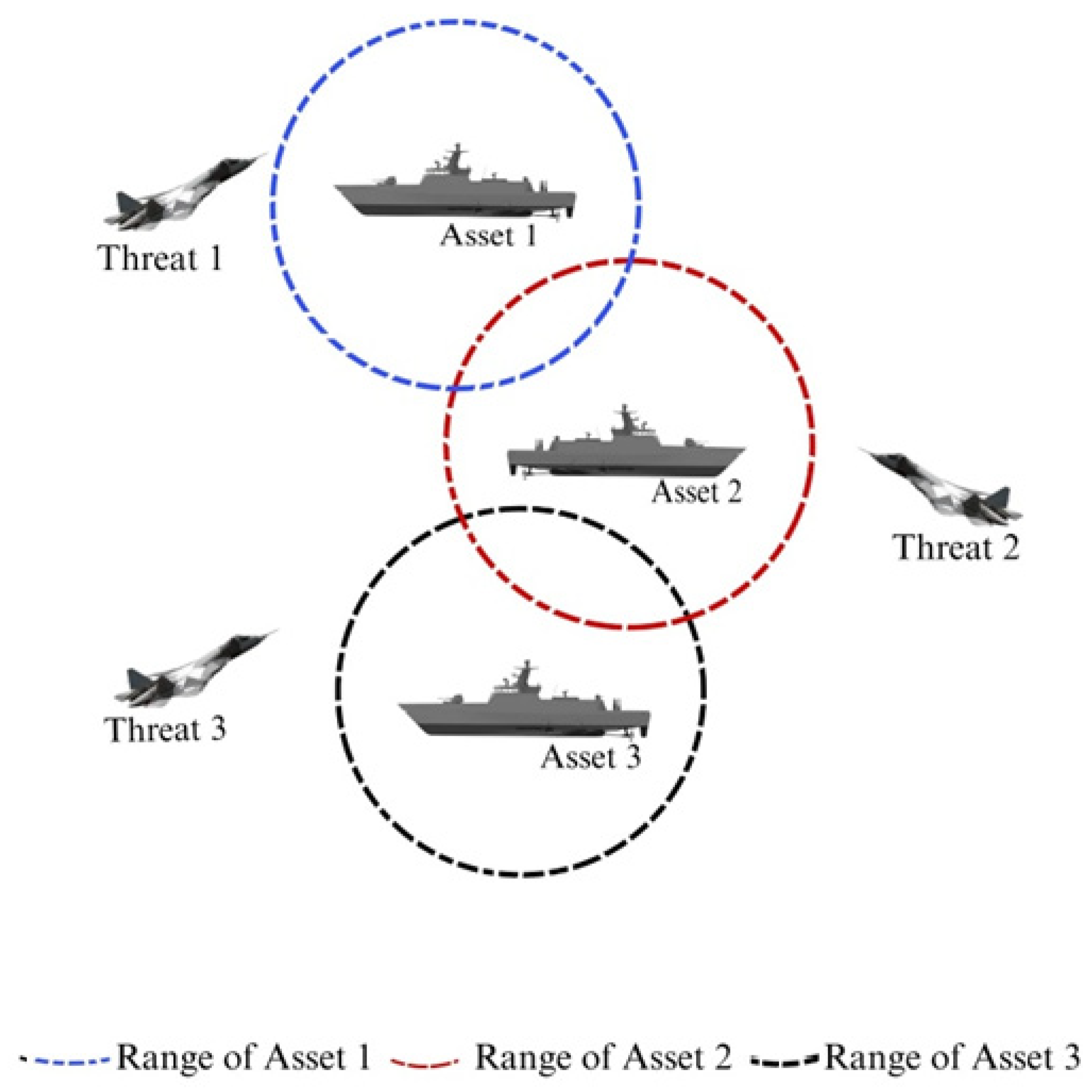
In this study, our primary objective is to develop an algorithm that effectively safeguards a naval fleet from aerial threats. Figure 1 illustrates an example of an aerial attack on a naval fleet. The circles in this Figure represent the vessels’ operational ranges. Defining these ranges is essential to manage computational complexity. The algorithm for the vessels need not consider threats beyond its specified range.
Figure 1.
An example for an aerial attack on a naval fleet.
During our experiments, we explored various scenarios, including different weapon types, varying weapon counts, threats approaching from different directions, and assets with diverse values. Additionally, we compared our results with a discrete dynamic weapon assignment approach.
Equation (1) is defined as a problem definition for asset-based systems. In Equation (1), is the probability that the weapon number kills the threat number . represents the probability of threat destroying the asset . represents the value of the asset since every asset may have a different importance level. Maximizing Equation (1) will maximize the survivability of the assets. The threats that want to destroy the asset are represented by . The assignment of weapon to target is represented with a binary value which is .
Using Equation (1), we derived a utility function as follows.
In Equation (2), there are additional parameters such as that represent the value of the threat and which represents the value of the cost of weapon . As one can see from Equation (2), as the probability of survival of the asset increases, the utility value also increases. On the other hand, the utility value decreases with the cost of the weapon.
We mentioned that we worked with a limited range for each vessel. We adapted a type of game from game theory called the dualist game [16]. Dualist game is described in [16] and modeled by a classic scene of two gunmen approaching each other. Here, the problem is which gunman shots first. The solution of this problem is that the gunman should fire his gun when the probability of the opponent of killing him will be higher than probability of him killing the opponent at the next step. Inequality in Equation (3) shows the adaptation of the dualist game for our application, and it is where our range is.
By the nature of the game theory, all units will try to maximize their utility. For a proper weapon assignment system, one needs an alignment with the vessels’ utility and the global utility. Potential games are introduced in [9] to align individuals’ utility to global utility. Consider vessels and targets , if is the set of vessels, and is the set of assignments, is the -th vessel, is the assignment of -th vessel, and is the assignment for all vessels except the -th vessel; then, the existence of Equation (4) means the existence of a potential game.
Equation (4) shows that any change in the strategy in function directly affects the vessels utility.
In [8], Arslan et al. introduces alignment functions. We combined Range Restricted Utility Function and Wonderful Life Utility Function, which is mentioned in [8]. According to Arslan in [8], Range Restricted Utility Function can be described as follows.
The main problem with Range Restricted Utility Function is that the defined area that defines a player’s range may overlap with that of another player. For overlapping areas, another alignment function must be defined. Therefore, we used Wonderful Life Utility Function with Range Restricted Utility Function for our simulations.
We use Wonderful Life Utility function. For Wonderful Life Utility Function, the vessels’ utility basically depends on its contribution to the global utility. Therefore, the vessels are forced to contribute to the global utility. In [8], Wonderful Life Utility is defined as follows.
Equation (6) shows that any change in the global utility will affect the vehicle’s utility in any change in assignments. Therefore, the function can be defined as a potential function. In other words, the vehicles must try to increase the global utility when they try to increase their own.
To obtain a continuous environment, we observed how the hit probabilities of ammunition changed over time depending on their range and the impact on the utility functions accordingly. For this purpose, we produced values for the time-varying hit probabilities of ammunition. To do this, we used the examples of real missiles given in [17] and the hit probability equations shown in [18], which are mentioned in detail below.
In the examples mentioned in [17], it was observed that the error rates of anti-tank missiles increased depending on the distance. Although these error rates are at their lowest when they are within the maximal and minimal ranges, they will increase as they approach these ranges and will reach their maximum as they begin to go outside these ranges.
When defining the error probability in firing and target hitting operations, Circular Error Probability (CEP) should be defined instead of defining the error probability in x and y axes in Cartesian coordinates. The probability of hitting a single shot should also be calculated by considering this error probability. In [18], the calculation of CEP values, Cookie Cutter Equations, and the probability of hitting a single shot are mentioned.
In [18], the damage function was defined to make these calculations. Here, if the distance between the weapon and the target is less than , the target will be hit. The probability of hitting the target, can be found by averaging the distance between the target and the weapon at the weapon’s final position. If is a two-variable function of the distance of the weapon relative to the target, it will be .
If the target is uniformly distributed over a large area , will be replaced by [18].
Since is defined as a large area, the definition will be approximately correct [18].
is the lethal area of the weapon in these equations [18]. At the same time, as seen here, the damage function is a function that does not increase. From here, it can be said that the weapons have a lethal area of diameter and the targets within this area will be hit. In this case, we can use the following equation to explain the meaning of the damage function.
The damage function is also differentiable. In this case, the probability distribution function can be obtained by differentiating [18].
For Cookie Cutter weapons, the lethal area is expressed as and is a constant. The lethal field is given by . If firing errors have the same standard deviation in all directions, the two-dimensional representation of the error density function is as follows [18].
In circular normal distribution, there is a relationship between CEP and as [18].
Analysis was made by considering the Cookie Cutter Equations in [19]. Equations (14) and (15) are obtained where is the angle of attack, is the height of the target, is the width of the target, and is the length of the target.
The assumption was made that a frontal or side approach would be equally likely. When the MATLAB erf function is set as follows, the possibility of hitting the target with a single shot of the ammunition emerges [19].
The erf function is defined as in MATLAB.
Here, changes to 1 and 2. Thus, it evaluates front and side views with an equal probability. is taken as . In this study, the probability of ammunition hitting the target was examined with this approach.
We give the pseudo code for the dynamic approach in Algorithm 1.
| Algorithm 1. Pseudo code for dynamic approach (ver. 1.4.2) | |
| 1: | for (Each Asset) |
| 2: | Define Utility Values of Weapons; Find Highest Value of Utility Function; Define Range; |
| 3: | end |
| 4: | if (Any Threat in Any Range) |
| 5: | Any Sharing Areas Defined Range |
| 6: | if (Single Asset Single Threat) |
| 7: | Fire Weapon; |
| 8: | else if (Multiple Asset Single Threat OR Multiple Asset Multiple Threat) |
| 9: | for (Each Asset Sharing Threat in Range) |
| 10: | Prepare Game Matrix; |
| 11: | Apply Alignment Function; |
| 12: | Find Nash Equilibrium; |
| 13: | Assign Weapon; |
| 14 | Fire Weapon; |
| 15: | else if (Single Asset Multiple Threats) |
| 16: | if (Any Threat in Any Range) |
| 17: | Fire Weapon; |
| 18 | end |
| 19: | end |
| 20: | end |
3. Proposed Approach
In the preceding sections, we introduced a naval system as the context for our weapon assignment problem. We also discussed the distinction between dynamic and static weapon systems. Notably, there is currently no truly dynamic approach for solving the dynamic weapon assignment problem, based on our best knowledge.
As previously mentioned, game theory offers a promising avenue for solving optimization problems in continuous environments. When game theory is employed, vehicles can operate independently, reducing both computation and communication burdens.
In co-operative games, aligning the utilities of players (in our case, the vehicles) is crucial. To achieve this alignment, we combined potential games with the Wonderful Life Utility Function and the Range Restricted Utility Function.
To address range limitations, we leveraged a concept from game theory known as the dualist game. In this approach, a vehicle should fire its weapon only when the probability of the threat killing it exceeds the probability of the vehicle eliminating the threat in the next step. Each vehicle’s weapon range is defined by inequality in Equation (3). If a threat lies outside a vehicle’s range, then, the vehicle is not considered a part of the game or solution, thus saving computational resources.
We further calculated Circular Error Probable (CEP) and Single Shot Hit Probability for the proposed weapons. These yielded continuous functions representing the relationship between distance and the probability of a hit for each weapon on the vehicles. By incorporating these functions into our utility calculations, we obtained continuous utility functions for each weapon.
The game theoretical solution aims to maximize the global utility function, which aggregates the utilities acquired from each target. Consequently, when a target reaches the point where the utility function peaks, the corresponding vehicle’s weapon shall fire.
4. Limitations of the Proposed Approach
Game theoretic approach for a dynamic weapon assignment system is a novel concept. Although we discussed some advantages of this approach, it also has some setbacks. First of all, any game theoretical approach heavily relies on personal choices and their reflection on a numerical plane. For example, in Equation (2), , which represents the value of the asset, and which represents the value of the threat, may not be objective values and may vary with the past experiences of the person who evaluates the situation.
This system is designed to be a part of a more complex system which is called Threat Evaluation and Weapon Assignment or TEWA. This study focuses solely on the weapon assignment problem. However, threats should have been evaluated and fed to the weapon assignment part of the system. Therefore, this study assumes the existence of an imaginary threat evaluation system, and the data that have been used by the weapon assignment system are provided by it. Additionally, this study does not take into account protective systems like electronic warfare equipment, as the threat evaluation system should handle them, and they are outside the scope of this study.
In a real-world combat zone, the information flow may not be perfect. The game theory can work with an environment with imperfect information. In fact, we studied the subject to extend our work here. However, our work on imperfect information is not yet ready to be presented. This study aims to present a new approach for dynamic weapon assignment systems, but we plan to conduct future research on systems with imperfect information.
The accuracy level of the weapons may change with the environmental conditions of the naval vessels. value in Equation (2) may vary with the conditions like wind and sea state.
5. Simulation Parameters
In this section, we discussed the simulation parameters. The simulation has been performed in the MATLAB environment. In the simulation, every vessel is also an asset. The vessels need to protect themselves as well as the other vessels.
In the classical solution of the dynamic system, time frames are used, and the optimization problem is solved in a similar way to the static system for the frames. We stated that one of our aims in this study was to change this method and find a solution to a truly dynamic situation. We also stated that weapon performance may vary depending on distance. The probability of error increases as the target approaches the minimum and maximum range limits. In the previous section, error probability was defined and the connection between error probability and hit probability was explained. In the previous sections, CEP and Single Shot Probability to Kill (SSPK) values were explained and how they were calculated was shown. This scenario will proceed through three weapon examples. It was assumed that one of these was a close-defense weapon. Therefore, the range of this weapon is quite short. At the same time, the SSPK value is lower than the others. The second weapon is considered as a medium range defense weapon. The SSPK value is at the medium level. The weapon with the highest SSPK value is considered a long-range weapon. For the three weapon examples, the three weapons have been chosen by these rules. Figure 2 shows the value of SSPK to CEP for the three weapon examples.
Figure 2.
SSPK value versus CEP of all weapons.
Figure 2 shows that, if CEP of all three weapons increases, then after a certain point (approximately 1 m for this example), the SSPK values will start to drop.
In this scenario, three threat examples were used. Threat #1 is the strongest and hardest to kill threat. Threat #2 is the medium-strength threat, and finally, Threat #3 is the weakest threat.
As can be predicted, when threats approach the weapons’ range limits, the CEP values of the weapons will increase. Therefore, the probability to kill decreases. For our scenario, we will show the kill probability for three threats and three weapons that vary depending on the distance of the threats.
Figure 3 shows the kill probability by distance of the three weapons for Threat #1. Figure 4 and Figure 5 show the probabilities of Threat #2 and Threat #3 being killed by the three mentioned weapons, respectively.
Figure 3.
Probability of killing Threat #1 of three weapons based on distance.

Figure 4.
Probability of killing Threat #2 of three weapons based on distance.
Figure 5.
Probability of killing Threat #3 of three weapons based on distance.
Figure 3 shows the probability to kill Threat #1 for all weapons. All weapons have a higher probability to kill within their range, and beyond their range, the probability to kill drops quickly. Weapon #1 has a higher probability to kill for all threats and has the highest range in terms of distance as can be seen in Figure 3, Figure 4 and Figure 5.
Figure 4 shows the probability to kill Threat #2 for all weapons. The probabilities are a little bit higher than those for Threat #1, because, as we mentioned, Threat #1 is the hardest to kill.
Figure 5 shows the probability to kill Threat #3 for all weapons. As one can see, the probabilities are the highest because, as we mentioned, Threat #3 is the easiest to kill.
Parameters used in Equation (2) are also needed when calculating the utility value. Table 1, Table 2, Table 3 and Table 4 show these values.

Table 1.
Probability of threat k destroying asset j, πjk.
Table 2.
Ammunition budget for weapon i, φi.
Table 3.
Asset values, ωk.
Table 4.
Threat values, Ωj.
Equation (2) was used to calculate utility values. Since only the probability of killing the threat from the weapons on the vehicles can be defined as a vector depending on distance and the other values are scalar, the probability of killing can be put into this equation as a vector. Thus, continuous utility functions are obtained depending on distance.
Figure 6 shows that the best weapon for Threat #1 is Weapon #1. Therefore, if this weapon fires against this threat, Weapon #1 should be fired, and it should be fired in the range of the minimum and maximum range limit of the weapon.
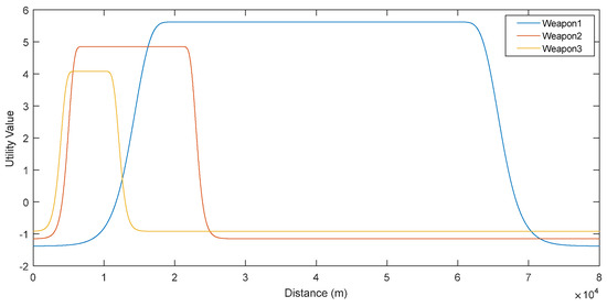
Figure 6.
Utility values against Threat #1.
Figure 7 shows that all three weapons are almost as effective as each other against Threat #2.
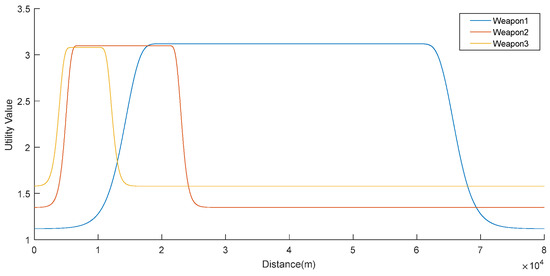
Figure 7.
Utility values against Threat #2.
Figure 8 shows that Weapon #3 has the best utility value against Threat #3. The system should wait until the threat comes as near as the range of Weapon #3.
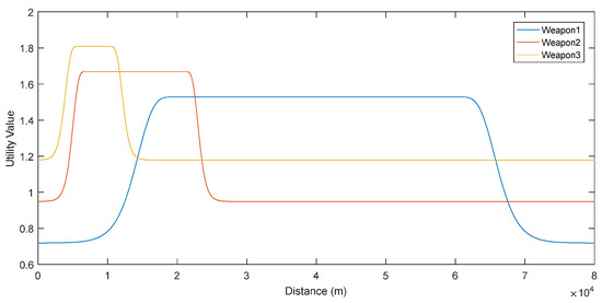
Figure 8.
Utility values against Threat #3.
It is clear that, by defining the utility function of the vessels as continuous functions, we can achieve a real dynamic system rather than a dynamic system defined by time frames. Using continuous utility values for individuals also perpetuates the global utility that is their combination. The maximum point of the global utility function will give the Nash Equilibrium. As can be seen in Figure 6, Figure 7 and Figure 8, each weapon defines its own range as a natural result of game theory. This creates the dynamic range limitation that we mentioned at the beginning. At the same time, by this way, we can easily see which threats these weapons are effective against. In this case, it becomes clear which threat which weapon should respond to and at what range. The difference between this and a time frame is that it not only shows the situation at that time step but also gives us an idea of the entire field. For example, in Figure 8, Threat #3 at 60,000 m can be engaged with Weapon #1 only when viewed at that time step. However, considering the entire field, waiting for this target to come to a closer range and engaging with Weapon #3 will have a larger utility.
To be perfectly clear, we will show an example for Threat #3 and Threat #1 incoming from 60,000 m, and they are at the range of two assets. Let us assume that the assets have the weapon sets of Weapon #1, Weapon #2, and Weapon #3. Following Algorithm 1, we need to prepare the game matrix. From Figure 6 and Figure 8, since they produce the highest utility value for Threat #3 and Threat #1, we already know that the best weapons for Threat #3 and Threat #1 are Weapon #3 and Weapon #1, respectively. Table 5 shows an example of the game matrix.
Table 5.
Example of game matrix.
From Table 5, one can see that the Nash Equilibrium is at [Threat #1, Threat #1] point. This is an unwanted result for us, since there is a better value for global utility. Following Algorithm 1, if we apply Wonderful Life Utility Function mentioned by Arslan et al. in [8], an asset can obtain as much as utility that they contribute to the global utility. Therefore, if both assets try to lock on Threat #1, only one of them can obtain the utility contribution. Hence, the game matrix changes as seen in Table 6.
Table 6.
Changed game matrix due to Wonderful Life Utility Function.
Table 6 shows that now the Nash Equilibrium is changed to [Threat #1,Threat #3] point. Now, the result is globally effective, and Asset #1 will shoot its Weapon #1 onto Threat #1 at 60,000 m, and Asset #2 will wait until Threat #3 gets closer, i.e., 15,000 m, to shoot its Weapon #3 onto Threat #3. More elaborated trials and results are given in the Section 6.
6. Results
The utility values of weapons that vary depending on distance are given in the previous sections. It is also mentioned that Range Restricted Utility Function and Wonderful Life Utility Function are used simultaneously to align the vessels’ utility value with the global utility.
Since distance is a value that affects the utility in the dynamic situation, weapons wait until the range where they provide the maximum utility. Therefore, the range at which the weapons were fired was also taken as a parameter in the simulations. Table 7 shows various dynamic case scenarios. All the scenarios use the three threats and the three weapons that we defined in previous chapters. On the other hand, some scenarios use more than one identical copy of Threat #1, Threat #2, or Threat #3. For example, the second scenario uses two identical threats like Threat #1.
Table 7.
Results of various scenarios.
The Section 6 shows how the trials ended. The vessel that has been chosen to fire its weapons against the threats may fire its weapons at different times. As it can be seen from Figure 6, if the chosen weapon is Weapon #1, then the vessel will fire its weapon when the threat is between 20,000 and 60,000 m away from the vessel. Similarly, if Weapon #2 is chosen, then the vessel should fire the weapon when the threat is between 5000 and 25,000 m away from the vessel, because, as it can be seen from Figure 6, Figure 7 and Figure 8, these are the optimum points for these vessels.
The maximum utility value is the sum of all utility values that have been gained from all threats for the scenario. Table 7 shows the results for various scenarios.
In Scenario #1, the vehicles have locked two weapons against two different threats. The first vehicle used Weapon #1 against Threat #1, and as shown in Figure 6, Weapon #1 is the optimum weapon for Threat #1. Weapon #1 has a range between 20,000 and 60,000 m; therefore, the vehicle fired Weapon #1 when the threat reached 60,000 m away from the vehicle. The other vehicle locked Weapon #3 to Threat #3. Weapon #3 has a range between 5000 and 10,000 m. Therefore, the vehicle waited to fire Weapon #3 until the threat was at an optimum distance for achieving the maximum utility. In cases where it is convenient to fire from the farthest distance, as in Scenario #2, the weapons choose 60,000 m. Since the number of defenders in Scenario #3 was greater than the number of threats, the maximum utility output was the same as in Scenario #2 because one of the defenders did not use any weapons or created any utility value. In Scenario #4, although both vehicles were initially loaded with two copies of Threat #1, and when Threat #3 came within the range of Weapon #3, one of the vehicles fired its Weapon #3. In Scenario #5, there are three Threat #1 and two vehicles, and since the threats are at a close range, the vehicles initially dealt with two of the threats. In this case, since they were still within range of Weapon #1, the most effective weapon, Weapon #1, was used. The last threat then moved out of Weapon #1’s range and one of the vehicles responded to the approaching threat with the second-best weapon, i.e., Weapon #2.
We compared our proposed method with the shoot–look–shoot (SLS) method for the dynamic case. As predicted, we saw differences in the solutions between the dynamic case and the proposed method depending on time frames. The applied scenario and the differences between the two methods are shown in Table 8.
Table 8.
Comparison between time frames and dynamic solution.
It can be seen that the scenarios that were used to test the algorithms in Table 7 and Table 8 are the same, making the comparison easier. In Table 8, Scenario #1 of Table 7 was repeated twice in the 1st and 2nd rows because different time frames gave different results. In the first case, the time frame was taken when the vehicles were at 60,000 m. Here, the most useful action for this time step is for both vehicles to fire their Weapon #1 towards two separate targets. However, it can be seen that the weapon that will actually bring the most utility for the second target is Weapon #3. However, it remains out of range at this time step. This results in a lower utility value obtained at this moment compared to that of the dynamic situation. In the second case, although the weapon that provides the highest utility is Weapon #3, the utility function decreases visibly in comparison with the dynamic situation. Scenarios #3 and #4 in Table 8 are the same as Scenarios #2 and #3 in Table 7. In these scenarios, it is seen that the maximum utility value in the dynamic and the time frame solution is the same. The frames taken are the points that already give the best results in the dynamic situation. Scenario # 5 in Table 8 is the same as Scenario #4 in Table 7. Here, two Threat #1 can be killed in the shown frame. However, one Threat #3 cannot be locked in the shown window. Therefore, there is a decrease in the total benefit value. The last scenario in Table 8 is the same as Scenario #5 in Table 7. In this scenario, although two Threat #1 can be destroyed in the shown frame, some targets cannot be destroyed in that frame because they are out of range. This causes a decrease in the utility value.
It can be seen from the examples that, since the entire field is considered in the dynamic case, the occurrence of a situation that will increase the utility values in the next steps cannot be observed in the statictime frames. This causes utility values to increase for Scenarios #1, #2, #5, and #6 for the dynamic weapon assignment systems.
7. Conclusions
In simulations conducted in a dynamic environment, the operation of different weapons at various ranges was analyzed. Each weapon is effective against different threats within its range. During the trials, it was observed that firing occurred at ranges that should be effective against each threat. Additionally, it was noted that, if the best weapon was occupied at that moment, the second-best weapon was also fired. If the threat moved out of the range of the best weapon, the second-best weapon was activated. In scenarios where the dynamic situation was compared with the time frame solution, it was observed that time frames had issues in seeing the whole picture, leading to a decrease in total utility for the static situation in some scenarios.
8. Future Research
It is known that, in a real-world combat zone, weapon assignment systems may deal with environments of imperfect information. Game theory is designed to handle such imperfect information. The system must assign types to threats based on beliefs and intelligence about the threats. Bayesian Nash Equilibrium will be the point of no regret for a system with imperfect information. However, this study focuses on a novel approach for dynamic weapon assignment systems. Although we have worked on imperfect information systems to expand our study, the study is still preliminary and not ready to be presented. Therefore, we consider it as future research.
Author Contributions
Conceptualization, O.A. and A.K.; methodology, O.A.; software, O.A.; validation, O.A. and A.K.; formal analysis, O.A.; investigation, O.A.; resources, O.A.; data curation, O.A.; writing—original draft preparation, O.A.; writing—review and editing, O.A. and A.K.; visualization, O.A.; supervision, A.K.; project administration, A.K. All authors have read and agreed to the published version of the manuscript.
Funding
This research received no external funding.
Data Availability Statement
The original contributions presented in the study are included in the article, further inquiries can be directed to the corresponding author.
Conflicts of Interest
The authors declare no conflict of interest.
References
- Paradis, S.; Benaskeur, A.; Oxenham, M.; Cutler, P. Threat Evalution and Weapon Allocation in Network-Centric Warefare. In Proceedings of the Seventh International Conferance on Information Fusion, Stockholm, Philadelphia, PA, USA, 25–28 July 2005. [Google Scholar]
- Roux, J.N.; Van Vuuren, J.H. Threat Evalution and Weapon Assignment Decision Support: A Review of the State of Art. ORiON 2007, 23, 151–187. [Google Scholar] [CrossRef]
- Lötter, D.P.; Van Vuuren, J.H. Weapon Assignment Decision Support in a Surface Based Air Defence Environment. Mil. Oper. Res. 2014. submitted. [Google Scholar]
- Glazebrook, K.; Washburn, A. Shoot-Look-Shoot: A Review and Extension. Oper. Res. 2004, 52, 454–463. [Google Scholar] [CrossRef]
- Johansson, F.; Falkman, G. Real-Time Allocation of Firing Units to Hostile Targets. J. Adv. Inf. Fusion 2011, 6, 187–199. [Google Scholar]
- Leboucher, C.; Shin, H.S.; Le Ménec, S.; Tsourdos, A.; Kotenkoff, A.; Siarry, P.; Chelouah, R. Novel Evolutionary Game Based Multi-Objective Optimization for Dynamic Weapon Target Assignmnet. In Proceedings of the 19th World Congress, The International Federation of Automatic Control, Cape Town, South Africa, 24–29 August 2014. [Google Scholar]
- Shi, Y.; Xing, Y.; Mou, C.; Kuang, Z. An Optimization Model Based on Game Theory. J. Multimed. 2014, 9, 583. [Google Scholar] [CrossRef]
- Arslan, G.; Marden, J.R.; Shamma, J.S. Autonomous Vehicle-Target Assignment: A Game-Therotical Formulation. J. Dyn. Sys. Meas. Control 2007, 129, 584–596. [Google Scholar] [CrossRef]
- Monderer, D.; Shapley, L.S. Potential Games. Games Econ. Behav. 1996, 14, 124–143. [Google Scholar] [CrossRef]
- Karasakal, O. Air Defense Missile-Target Allocation Models for a Naval Task Group. Comput. Oper. Res. 2006, 35, 1759–1770. [Google Scholar] [CrossRef]
- Hammond, L. Application of a Dynamic Programming Algorithm for Weapon Target Assignment; Weapons and Combat Systems Division, Defence Science and Technology Group: Edinburgh, Australia, 2016; DST Group-TR-3221. [Google Scholar]
- Taghavi, R.; Ranjbar, M. Weapon Scheduling in Naval Combat Systems for Maximization of Defense Capabilities. Iran. J. Oper. Res. 2015, 6, 87–99. [Google Scholar]
- Yang, Y.; Wang, F.Y. Budget Constraints and Optimization in Sponsored Search Auctions; Academic Press: Cambridge, MA, USA, 2014. [Google Scholar]
- Hosein, P.A. A Class of Dynamic Nonlinear Resource Allocation Problems. Doctoral Thesis, Massachusets Instıtude of Technology, Boston, MA, USA, 1989. [Google Scholar]
- Galati, D.G. Game Theoretic Target Assignment Strategies. Doctoral Thesis, University of Pittsburg, Pittsburgh, PA, USA, 2002. [Google Scholar]
- Gupta, M.; Sharma, B.; Tripathi, A.; Singh, S.; Bhola, A.; Singh, R.; Dwivedi, A.D. n-Player Stochastic Duel Game Model with Applied Deep Learning and Its Modern Implications. Sensors 2022, 22, 2422. [Google Scholar] [CrossRef] [PubMed]
- U.S. Defence Documentation Center. Scientific and Technical Information; U.S. Defence Documentation Center: Alexandria, VA, USA, 1963.
- Washburn, A.R. Notes on Firing Theory; Naval Post Graduate School: Monterey, CA, USA, 2002. [Google Scholar]
- Wonnacott, W.M. Modelling in the Design and Analysis of a Hit-To-Kill Rocket Guidance Kit. Master Thesis, Naval Postgraduate School, Monterey, CA, USA, 1997. [Google Scholar]
Disclaimer/Publisher’s Note: The statements, opinions and data contained in all publications are solely those of the individual author(s) and contributor(s) and not of MDPI and/or the editor(s). MDPI and/or the editor(s) disclaim responsibility for any injury to people or property resulting from any ideas, methods, instructions or products referred to in the content. |
© 2024 by the authors. Licensee MDPI, Basel, Switzerland. This article is an open access article distributed under the terms and conditions of the Creative Commons Attribution (CC BY) license (https://creativecommons.org/licenses/by/4.0/).