Article

Population Balance and CFD Simulation of Particle Aggregation and Growth in a Continuous Confined Jet Mixer for Hydrothermal Synthesis of Nanocrystals

1
School of Chemistry and Chemical Engineering, South China University of Technology, Guangzhou 510641, China
2
Pharmaceutical and Crystallization Systems Engineering Group, Beijing Key Laboratory of Enze Biomass and Fine Chemicals, School of Chemical Engineering, Beijing Institute of Petrochemical Technology, Beijing 102617, China
*
Author to whom correspondence should be addressed.
Crystals 2021, 11(2), 144; https://doi.org/10.3390/cryst11020144
Submission received: 2 January 2021 / Revised: 22 January 2021 / Accepted: 25 January 2021 / Published: 29 January 2021

Abstract

:
Population balance and computational fluid dynamics models are built and integrated to carry out a simulation study of the reactive crystallisation process in a confined jet mixer (CJM) for the continuous flow synthesis of TiO2 nanoparticles at a supercritical water condition. In the population balance model, the crystal growth in size is modelled as being due to combined nanocrystal aggregation as well as surface growth. A free molecular model is used to predict the particle aggregation. The performance of the combined aggregation and surface growth models is compared with models that only consider surface growth as the only mechanism for particle size enlargement. It was found that the combined model gives a more accurate prediction of particle size distribution.

1. Introduction

Continuous hydrothermal flow synthesis (CHFS) of nanoparticles below 100 nm in size has shown numerous advantages [1,2,3,4,5]. It is considered as a green technology as it uses water as a reagent rather than organic solvents. In addition, since it is operated in continuous mode instead of batch [2,3,4], it is much easier to control, avoiding batch to batch variation. The mixing and heat transfer are clearly critical inside the CHFS reactor, i.e., the impinging jet mixer, and therefore, these factors have received a great deal of attention from researchers, who have applied computational fluid dynamics (CFD) simulation in their studies on the CHFS process. In some of the CFD simulation studies, solid particles were either completely excluded from the modelling and simulation [5,6], or simplified as a mono-disperse system, i.e., all particles are assumed to have an equal diameter [7]. Accurate CFD simulation should take into consideration the reactive crystallisation process by incorporating population balance models (PBM). In our previous study, Chen et al. [8] used gPROMS to build PBM models to predict the particle size distribution, in which, the reactor was modelled as a continuous mixed-suspension, mixed-product-removal (MSMPR) reactor. In a study on CuO and ZnO nanoparticle synthesis in a CHFS process, Zhou et al. [9] and Leybros et al. [10] integrated CFD and PBM simulations, in which crystal growth was modelled as being due to surface growth. In another study of CFD applications to a CHFS process [11], preliminary integration of CFD with PBM was also attempted, but the crystallisation model was only based on the surface growth without considering aggregation, and the simulation result on PSD was not validated using experimental data.
The current study is based on an observation by several researchers [12,13] on the mechanism of crystal growth during rapid reactive crystallisation. Specifically, that crystal size enlargement might not be wholly due to surface growth, and fine particle aggregation could play a more important role. Erriguible et al. [13] believed that particle growth in CHFS, especially for those processes which produce metal nanoparticles, could be mainly governed by coalescence and aggregation mechanisms instead of surface growth. They used a mono-disperse CFD model to predict mean particle size in the reactor. However, the actual PSD could not be obtained from the modelling strategy as the particles were assumed to be mono-dispersed.
The focus of the current work is on study of the effect of aggregation model in combined CFD and PBM simulation of the CHFS process. Simulations were carried out in two scenarios: (1) particle enlargement due to particle growth only, i.e., based on the surface growth theory, without considering aggregation, (2) due to both surface growth and aggregation. The simulation study is for a specific reactor design, i.e., the confined jet mixer (CJM). This is because in a previous study, Ma et al. [11] compared a counter-current mixer (CCM) with CJM and concluded that CJM offered more effective mixing between supercritical water and precursor streams than CCM.

2. Coupled CFD–PBM Model

2.1. Mathematical Formulation

In the coupled CFD–PBM simulation, the CFD hydrodynamic model developed by Ma et.al [11] is used. The CFD model interacted with: (a) chemical species transport equations for determining the species concentrations before nucleation; (b) chemical reaction equations to simulate the formulation reaction of metal oxide; and (c) user defined functions of nucleation, growth, and aggregation, along with the PBM model to predict particle size distribution (PSD). All calculations were carried out using ANSYS Fluent 13.0 software. For readability purposes, the CFD model is still briefly descried here.

2.1.1. Meshing

As a preliminary step for the proposed study, the computational domains of the CJM reactor with discretized cells were produced using the Gambit 2.4 software. The computational domain of the confined jet reactor was discretized with 2.96 × 10⁵ tetrahedral cells, including a stainless-steel inner tube for introducing supercritical water to the mixing point, and an outer tube with precursor stream being introduced radically via two inlet arms and flowing upwards in the annual channel between the inner and outer tubes. The flow field and mixing domains were three dimensional, and have been tested by mesh independence analysis, with the reactor meshing being validated through the comparisons between the predicted and measured temperatures in the non-reacting hydrodynamics studies, as reported previously in Ref. [11]. Although anisotropic mesh adaptivity is considered optimum for transient CFD problems [14], since the simulation here is a steady computational model, fixed meshes were sufficient, as the result in this work indicated.

2.1.2. Thermodynamic and Material Property

The thermodynamic and material properties of water including density, viscosity, thermal conductivity and specific heat at high temperature and pressure conditions were calculated using the International Association for the Properties of Water and Steam (IAPWS) formulation 1995 [11]. Since the mathematical formulation contains a large amount of special functions, it will be too computationally expensive to solve the IAPWS equation. In this work, the method reported by Ma et al. [5] was used to simplify the calculation. In the current study, the feed concentration of metal salt precursor solution is relatively low (0.1 M) and the typical solid concentrations in the nanoparticle slurries were under 0.1% w/w, as reported in previous experimental studies [15,16]. Therefore, it is reasonable to assume that the system is relatively dilute, so the effects that metal species present on inlet feeds can be ignored [11]. Based on this assumption, the properties of metal species were assumed to be the same as those of water. The chemical composition of the mixture solution was calculated using species transport equations of a multiphase model, and will be presented in Section 2.1.3. The thermodynamic constants for calculating solubility and the supersaturation of metal species were obtained using the same method described in our previous work [8].

2.1.3. Hydrodynamics

The products produced by a CHFS process are hot suspensions or slurries with relatively low solid concentrations (<1% in this case study), produced in a few seconds. As mentioned above, the properties of metal species were assumed to be the same as those of water. So, it is reasonable to adopt a non-reacting hydrodynamics study here. Therefore, the flow regime of the system should be characterized as liquid–solid multiphase flow. The Eulerian–Eulerian multiphase approach, which adopts the concept of phase volume fraction and treats each phase as one interpenetrating continua, was selected for the numerical calculation of this work. With this method, the primary phase was assumed to be a mixture between supercritical water, room temperature water for dilution, precursor solution and intermediate liquid phase metal species, whereas the particulate phase was considered as a dispersed secondary phase. The volume of each phase was defined by its phase volume faction:
V i = V α i d V
where α i is the volume fraction of phase i, and
i = 1 n α i = 1
The governing equations for the Eulerian–Eulerian multiphase model are listed as follows:
The Continuity Equation
t ( α P ρ P ) + × ( α P ρ P v P ) = P = 1 2 ( m P S m S P )
where is the v P is the velocity of primary phase and m P S characterizes the mass transfer from the primary phase to secondary phase, the reverse is likewise.
The Momentum Balance Equation
t ( α P ρ P v P ) + × ( α P ρ P v P v P ) = α P P + Γ = P + α P ρ P g + P = 1 2 ( F v m , P + m S P v S P m P S v P S ) + ( F P + F l i f t , P + F i n , P )
where Γ = P is the primary phase stress–strain tensor
Γ = P = α P μ P ( v P + v P T ) + α P ( λ P 2 3 μ P ) × v P I =
and μ P and λ P are the shear and bulk viscosities of the primary phase, F P is the external body force, F l i f t , P is the lift force, F v m , P is the virtual mass force, F i n , P is the inter-action force between phases and P is the pressure shared by all phases. In most cases, external body force and lift force are not significant and can be neglected from computations. Additionally, the virtual mass force is only important when the density of the secondary phase is much smaller than the primary phase. Therefore, this source term can also be neglected from Equation (5). v P S is the interphase velocity. If m P S > 0 (i.e., the primary phase mass is being transferred to the secondary phase), then v P S = v P and if m P S < 0 (i.e., the secondary phase mass is being transferred to the primary phase), then v P S = v S .
The solution of Equations (1)–(5) for one phase, along with the theory that the sum of phase volume fractions is equal to one, allows for the calculation of the volume fraction of another phase.

Energy Balance Equation

The energy balance is given by the standard energy equation as:
t ( ρ E ) + × ( v ( ρ E + P ) ) = × ( k e f f T j h j J j + ( τ = e f f × v ) )
where k e f f is the effective conductivity which depends on the turbulence model, J j is the diffusion flux of species j that includes Fickian diffusion, Fourier conduction and Soret–Dufour effects.

The Turbulence Model

In comparison to single-phase flows, modelling turbulence in a multiphase system is much more complex due to the addition of a large quantity of momentum equations of all phases. Among the several turbulence models available in ANSYS Fluent package, the standard k-ε model was selected to model turbulence in the CFD–PBM coupled model because of previous work in the modelling turbulence for non-reacting CFD simulation of the same CHFS systems [11]. Turbulent kinetic energy k and its dissipation rate ε are the two quantities for which two additional transport equations (Equations 7 and 8) are solved with standard empirical constants given by Launder et al. [17].
t ( ρ k ) + x i ( ρ k μ i ) = x j [ ( μ + μ t σ k ) k x j ] + G k + G b ρ ε Y M
t ( ρ ε ) + x i ( ρ k μ i ) = x j [ ( μ + μ t σ ε ) ε x j ] + G 1 ε ε k ( G k + C ε 1 G b ) C ε 2 ρ
with the turbulence viscosity μ t is defined as:
μ t = 0.09 ρ k 2 ε
where G k represents the generation of turbulence kinetic energy due to the mean velocity gradients, G b is the generation of turbulence kinetic energy due to buoyancy, Y M represents the contribution of the fluctuating dilatation in compressible turbulence to the overall dissipation rate, σ k and σ ε are the turbulent Prandtl numbers for k and ε. The four empirical constants, σ k , σ ε , C ε 1 , C ε 2 , are determined by matching experimental data for simple turbulent flows with typical values of σ k = 1, σ ε = 1.3, C ε 1 = 1.44 and C ε 2 = 1.92 [15,18]. These default values were determined from experiments for fundamental turbulent flows including frequently encountered shear flows like boundary layers, mixing layers and jets as well as for decaying isotropic grid turbulence. They were found to work well for a wide range of wall-bounded and free shear flows.

2.1.4. Mixing and Reaction Model

Simulation of mixing in the non-reacting CFD model was carried out by introducing an inert tracer that has the same property as supercritical water (SCW), into the bulk SCW phase in the reactor. The tracer was treated as the secondary phase and the SCW was therefore considered to be the primary phase liquid. The tracer concentration and residence time distribution was solved using the Reynolds-averaged species transport Equation [11]:
ρ Y i t + ρ μ j Y i x j = x i ( Γ i , e f f Y i x j )
where the effective diffusion coefficient of species i, Γ i , e f f = Γ i + μ i / S c t , ρ is the mixture density, ui is the mixture velocity, Yi represents the species mass fraction, Γi the species diffusion coefficient, μt the turbulent eddy viscosity.
In the coupled CFD–PBM model, the composition of mixture components in the primary phase was determined by coupling Equation (10) with a reaction model (see description below) used for solving the hydrothermal reaction. The properties of the mixture used in the calculation were defined by volume/mass weighted mixing laws for mixture components and are described as follows:
ρ = 1 i Y i ρ i
c p = i Y i c p , i
k = i Y i k i
μ = i Y i μ i
where Y i , ρ i , c p , i , k i and μ i represent the mass fraction, density, specific heat capacity, thermal conductivity, and viscosity of species i, respectively. The diffusion coefficient of mixture was solved by a modified Chapman–Enskog equation and was dependent on the mixture temperature [19].
The hydrothermal reaction of this study contains a hydrolysis step (Equation (15)) and dehydration step (Equation (16)):
[ C H 3 C H ( O ) C O 2 N H 4 ] 2 T i ( O H ) 2 + 4 H 2 O T i ( O H ) 4 + 2 H 10 C 6 N O 4
T i ( O H ) 4 T i O 2 + 2 H 2 O
The hydrolysis reaction is considered as the dominant step [20] and the produced intermediate is quickly consumed and transfers to liquid phase titanium metal oxide. Therefore, the hydrothermal reaction can be simplified as a one-step reaction in the form of A + sB C. With this assumption, the composition of mixture species after hydrothermal reaction was determined by adding a reaction source term to the mixing model. Thus, Equation (10) was converted to:
ρ Y i t + ρ μ j Y i x j = x i ( Γ i , e f f Y i x j ) + R i
where R i is the net reaction rate of specie i. For an irreversible reaction, R i is defined as:
R i = Γ ( v i , p v i , r ) [ κ f i = 1 N ( C i ) ( η i , r + η i , p ) ]
where v i , p , v i , r , η i , p and η i , r are the stoichiometric coefficient and rate exponent for product and reactant species, respectively; C i is the molar concentration of species, and κ f is the reaction rate constant given by an Arrhenius expression:
κ f = A r T × e ( E r / R T )
where, the pre-exponential factor A r and the activation energy E r were obtained from the literature data [21].

2.1.5. Population Balance Model

In order to take into account the particles present in the simulation, a number density function was introduced into the coupled CFD–PBM models. Here, the number density of particles is defined as the total number of particles per unit volume. The number density function can be calculated from the population balance equation using a number of possible solution methods such as the homogeneous discretization method [22,23], the standard method of moments (SMM) [24], and the quadrature method of moments (QMOM) [25,26]. The discrete method is able to directly compute the particle size distribution and is particularly useful if the particle size range is known. However, it can be computationally expensive if the size distribution is wide, hence, a large number of equations is needed to achieve accurate predictions. The SMM method can save the computational cost by solving average transport equations of moments rather than the actual size distribution quantities. The PSD can be reconstructed from the calculated moments based on the “statistically most probable” distribution. The disadvantage of the SMM method is that with limited numbers of calculations, the model outcome may not be adequate to describe the real PSD. Additionally, it cannot be used for the cases with size-dependent aggregation and growth. The QMOM method is an alternative to SMM that eliminated the limitations of size-independency calculation. However, components mass transfer during the nucleation stage is neglected in the calculation procedure of QMOM, therefore in practice, for processes such as crystallization, where particle birth is due to nucleation, an initial value of nuclei mass needs to be patched into the system at the beginning of the simulation. This operation will increase the uncertainties of the accuracy of predictions. In this work, the average particle size range can be estimated from literature [12,27,28,29,30,31], therefore, the discrete method was chosen to solve the PBM equation in the coupled CFD–PBM model.
In the discretized method, the particles are discretized into a finite numbers of size classes or bins. As with the same treatment of the primary phase in the Eulerian–Eulerian multiphase model, the PB equation is written in terms of volume faction of particles as:
t ( ρ s α i ) + ( ρ s μ i α i ) + V ( G v ρ s α i V ) = ρ s V i ( B a g , i D a g , i + B b r , i D b r , i ) + 0 i ρ s V 0 n 0
where ρ s is the density of the secondary phase; α i is the volume fraction of particles size i and is defined as:
α i = N i V i         i = 0 , 1 , , N
with N i as the local number density function expressed as:
N i ( t ) = V i V i + 1 n ( V , t ) d V
where V i is the volume of particle size i.
The n 0 and V 0 in (Equation (20)) represent the nucleation rate and the volume of the smallest particle size, respectively. G v is the growth rate of particles that is discretized as:
V ( G v ρ s α i V ) = ρ s V i [ ( G v , i 1 N i 1 V i V i 1 ) ( G v , i N i V i + 1 V i ) ]
The mass transfer from liquid to solid phase ( T i O 2 ( a q ) T i O 2 ( s ) ) was simulated by:
m = ρ V 0 n 0 + i ρ G v , i N i
in which, all parameters related to the nucleation and growth terms were the same as those used in the PBM model described in our previous study [8,28,29].
The terms B a g , i , D a g , i , B b r , i and D b r , i in (Equation (20)) represent the birth and death rate of particles due to aggregation and breakage, respectively. In this work, it was assumed that no particle breakage occurred during the production. Therefore, B b r , i and D b r , i were eliminated from the PB equation. The two aggregation terms are defined as:
B a g = 1 2 0 V a ( V V , V ) n ( V V ) d V
D a g = 0 a ( V , V ) n ( V ) n ( V ) d V
where particles of volume (VV′) aggregate with particles of volume V′ to form particles of volume V.
Several models are available in ANSYS Fluent to simulate the aggregation kernel a ( V , V ) in (Equations (25) and (26)). The Luo model [32] and turbulent aggregation kernel [33,34] are highly dependent on the accurate prediction of the local shear rate and are independent to particle size. Therefore, they are not suitable for the current study. The free molecular model uses the Brownian kernel function [35] with the consideration of size effects on particle collision. For submicron particles, Testino et al. suggested that the Brownian kernel function would be more appropriate [36]. Peukert et al. also concluded that the Brownian motion is one of the most important transport mechanisms for nanoparticles and submicron particles [37].
Therefore, the free molecular model was selected for predicting particle aggregation in the coupled CFD–PBM simulations.

2.2. Numerical Procedure

The computational domain of the CJM reactor was discretized as 2.96 × 10⁵ tetrahedral cells, as shown in Figure 2b. The hydrodynamics and mixing behaviour and the particle size distribution in both the CHFS systems were studied based on the operating conditions descripted in Section 3.
The PBM equation was coupled with CFD using the Sauter mean diameter D3,2 (surface-area average diameter) approach as defined in Equation (10).
D 3 , 2 = 1 N × i = 1 N N i D i 3 i = 1 N N i D i 2
where D is the particle diameter and N total number of particles.
The homogeneous discretisation method was used to solve the PBM equations. For the particle no aggregation mode, the obtained TiO2 nanoparticles were classified into ten size ranges from 1 to 512 nm. For the particles with aggregation mode, the size was up to 4 µm [12,27,28,29,30,31]. In order to calculate the particle size distributions, the obtained TiO2 nano particles were first expressed by the Sauter mean diameter (D3,2) (Equation (27)) and then, converted into the length mean diameters (D1,0), as described below.
D 1 , 0 = 1 N × i = 1 N N i D i
The mass, momentum and energy conservation equations and species transport equation, together with the equations for turbulent quantities, k and ε, were solved using ANSYS Fluent software (2010) to obtain the velocity, temperature and turbulence viscosity in the confined jet mixer. Turbulence viscosity. The species equations were solved with the steady-state flow and temperature profiles obtained as the initial values. The equations were numerically solved using the finite volume method. The standard SIMPLE pressure–velocity solver was employed, coupled with a first-order upwind scheme for the discretisation of the convection terms in the governing equations. Note that the heat loss of the system was negligible (i.e., an adiabatic boundary condition). The mass inlet flow mode was used to calculate the inlet velocities from each stream at constant temperatures. The outlet boundary was defined as the pressure outlet with the temperature obtained from the blank CFD simulation [10]. A typical turbulent intensity (5%) with the corresponding hydraulic diameters was used for the inlet conditions for the CFD–PBM turbulence analysis. Standard non-slip wall boundary conditions were applied with a standard turbulent wall function. Solution convergence was achieved once the energy residuals were less than 10−6 and the other residuals were lower than 10−3 for all simulations.

3. Comparison and Validation

The experimental data of our collaborator Weng et al. [38] was used for validation purposes. The experimental rig is shown in Figure 1. Deionized water was heated to 723 K and pumped into CJM reactor by pump P1 at a constant flow rate of 30 mL/min. A stream of aqueous precursor TiBALD solution (0.1 M, pumping rate at 7.5 mL/min) was pumped into the CJM reactor using pump P2 and a flow of deionized water (pumping rate at 7.5 mL/min) was pumped through P3 at room temperature, respectively. The system pressure was maintained at 23.1 MPa. The obtained TiO2 nanoparticles travelled upwards for rapid cooling before harvest.
ImageJ was used to extract particle size information from TEM images in Weng et al. [38]. The measuring scale was configured equal to the length scale given by TEM. Over 200 particles were counted and analyzed. All the data formed a histogram to compared with the predicted PSD.
The CJM reactor was designed with an inner tube (Di = 0.99 mm), inserted upwards into a larger tube (Di = 4.57 mm), with two horizontal feeder arms attached on both sides, as shown in Figure 2a. Ten long, fine J-type thermocouples were inserted at different locations along the z direction in order to control and modify the temperatures within the CJM reactor [11]. The precursors flowed horizontally into the CJM reactor to mix and react with the supercritical water at the reaction zone, as shown in Figure 2. The computational domain of the CJM reactor was discretized as 2.96 × 10⁵ tetrahedral cells, as shown in Figure 2b.

4. Result and Discussion

The velocity vector at the CJM reaction zone using the particles without aggregation simulation mode is shown in Figure 3a. In comparison, the velocity vector with a less pronounced recirculation behavior is shown in Figure 3b using the particles with aggregation simulation mode. This may be due to the gravity effect and the higher viscosity of TiO2 aggregation presented within the suspension.
As shown in Figure 4, the temperature in the CJM reactor rapidly reached to the equilibrium conditions after the streams mixing process. High temperatures above 550 K were observed in the majority of the flow fields. This assured the reduction in the species solubility and hence, increased the nucleation and particle precipitation rates [3]. The outlet temperature of the CJM reactor was calculated as about 550 K for both the particle presented only mode and the particles with aggregation mode, as shown in Figure 4a,b. However, because the CJM reactor rapidly reached the equilibrium conditions, the impacts to the overall flow temperature were negligible within the system.
High turbulence viscosity was observed in the center of the reaction zone. As shown in Figure 5a,b, the maximum value of the turbulence viscosity increased to 1.82 × 10⁻² Kg/m·s in both modes. Note that less uniformly distributed turbulence viscosity was observed due to the TiO2 nanoparticles aggregation which enhanced the turbulent disturbance as a result of more complicated particles flow phenomenon appeared within the CJM reactor.
The particle size distribution (PSD) obtained from CFD–PBM modelling is shown in Figure 6 and Figure 7. Figure 6 showed the particle size distribution contour at the system outlet. The obtained particles appeared to be uniformly distributed at the cross-sectional outlet surface when using the particles with no aggregation simulation mode, as shown in Figure 6a. Note that a small amount of large TiO2 nanoparticles was observed near the CJM reactor wall (light yellow areas). On the other hand, larger particle size was observed at the cross-sectional outlet surface when the particle aggregation phenomenon was involved in the simulation analysis, as shown in Figure 6b. Large particles observed near the CJM reactor wall are not only due to the low flow velocity of this area during production process, but also because of the collision of particles with the tube wall. This may potentially lead to accumulations of particles and agglomerates in this area.
The mean predicted particle size was about 4 nm when using the particles with no aggregation simulation mode, as shown in Figure 7a. Narrow particle size distribution was obtained in this simulation mode. The mean predicted particle size was about 8 nm when aggregation was considered during simulation, as shown in Figure 7b. Larger TiO2 nanoparticles with broader particle size distributions, obtained when involving aggregation effects, were probably related to the size dependence of the Brownian aggregation kernel, as smaller particles were more likely to collide and produce large aggregates [35,39].
As shown in Figure 8, the PSD obtained with aggregation was compared with published experimental data [38], which showed good agreement. As we can see from the experimental data histogram, most of the particles were larger than 5 nm. With no aggregation mode, the simulation result showed that mean predicted particle size was about 4 nm which is inconsistent with the experimental results. It can be inferred that aggregation phenomenon exists in the particle growth process.

5. Conclusions

The study on the combined population balance and computational fluid dynamics simulation has proved that it is important to take into consideration not only surface growth, but also aggregation as the mechanisms of crystal growth in a confined jet mixer (CJM) for the hydrothermal synthesis of nanomaterials. The hydrodynamic and thermodynamic variables, including velocity, temperature and mixing in a CJM reactor configurations were simulated. The particle aggregation was found to play an important role in the CJM TiO2 nanoparticle production process. The free molecular model with the Brownian kernel function was chosen to describe the size effects on particle collision during aggregation. When considering aggregation, the simulation result showed a lower mixing velocity and higher turbulence viscosity compared with the no aggregation condition. The aggregation effect on temperature is not obvious. According to the simulation result, without aggregation, the mean particle size is about 4nm and the PSD is narrow. When considering aggregation, the mean particle size is about 8nm and the PSD becomes wider. The simulated PSD result, when considering aggregation, is more consistent with the published experimental data.

Author Contributions

Conceptualization, X.Z.W. and Q.Y.L.; methodology, Q.Y.L. and X.Z.W.; software, Q.Y.L.; validation, Q.Y.L. and X.Z.W.; formal analysis, Q.Y.L. and X.Z.W.; investigation, Q.Y.L.; resources, X.Z.W.; data curation, Q.Y.L.; writing—original draft preparation, Q.Y.L.; writing—review and editing, X.Z.W.; visualization, Q.Y.L.; supervision, X.Z.W.; project administration, X.Z.W.; funding acquisition, X.Z.W. All authors have read and agreed to the published version of the manuscript.

Funding

This research received financial support from the National Natural Science Foundation of China (NNSFC) (grant numbers: 61633006 and 91434126), the Guangdong Provincial Science and Technology Projects under the Scheme of Applied Science and Technology Research Special Funds (grant number: 2015B020232007), and the Open Project Program of the Beijing Key Laboratory of Enze Biomass & Fine Chemicals, Beijing Institute of Petrochemical Technology.

Conflicts of Interest

The authors declare no conflict of interest.

References

  1. Darr, J.A.; Zhang, J.; Makwana, N.M.; Weng, X. Continuous Hydrothermal Synthesis of Inorganic Nanoparticles: Applications and Future Directions. Chem. Rev. 2017, 117, 11125–11238. [Google Scholar] [CrossRef] [Green Version]
  2. Adschiri, T.; Hakuta, Y.; Arai, K. Hydrothermal Synthesis of Metal Oxide Fine Particles at Supercritical Conditions. Ind. Eng. Chem. Res. 2000, 39, 4901–4907. [Google Scholar] [CrossRef]
  3. Adschiri, T.; Kanazawa, K.; Arai, K. Rapid and Continuous Hydrothermal Crystallization of Metal Oxide Particles in Supercritical Water. J. Am. Ceramic Soc. 1992, 75, 1019–1022. [Google Scholar] [CrossRef]
  4. Darr, J.A.; Poliakoff, M. New Directions in Inorganic and Metal-Organic. Co-ordination Chemistry in Supercritical Fluids. Chem. Rev. 1999, 99, 495–541. [Google Scholar] [CrossRef] [PubMed]
  5. Ma, C.Y.; Tighe, C.; Gruar, R.I.; Mahmud, T.; Darr, J.A.; Wang, X.Z. Numerical modelling of hydrothermal fluid flow and heat transfer in a tubular heat exchanger under near critical conditions. J. Supercrit. Fluids 2011, 57, 236–246. [Google Scholar] [CrossRef]
  6. Demoisson, F.; Ariane, M.; Leybros, A.; Muhr, H.; Bernard, F. Design of a reactor operating in supercritical water conditions using CFD simulations. Examples of synthesized nanomaterials. J. Supercrit. Fluids 2011, 58, 371–377. [Google Scholar] [CrossRef]
  7. Kawasaki, S.-I.; Sue, K.; Ookawara, R.; Wakashima, Y.; Suzuki, A.; Hakuta, Y.; Arai, K. Engineering study of continuous supercritical hydrothermal method using a T-shaped mixer: Experimental synthesis of NiO nanoparticles and CFD simulation. J. Supercrit. Fluids 2010, 54, 96–102. [Google Scholar] [CrossRef]
  8. Chen, M.; Ma, C.Y.; Mahmud, T.; Darr, J.A.; Wang, X.Z. Modelling and simulation of continuous hydrothermal flow synthesis process for nano-materials manufacture. J. Supercrit. Fluids 2011, 59, 131–139. [Google Scholar] [CrossRef]
  9. Zhou, L.; Wang, S.; Xu, D.; Guo, Y. Impact of Mixing for the Production of CuO Nanoparticles in Supercritical Hydrothermal Synthesis. Ind. Eng. Chem. Res. 2013, 53, 481–493. [Google Scholar] [CrossRef]
  10. Leybros, A.; Piolet, R.; Ariane, M.; Muhr, H.; Bernard, F.; Demoisson, F. CFD simulation of ZnO nanoparticle precipitation in a supercritical water synthesis reactor. J. Supercrit. Fluids 2012, 70, 17–26. [Google Scholar] [CrossRef]
  11. Ma, C.Y.; Chen, M.; Wang, X.Z. Modelling and simulation of counter-current and confined jet reactors for hydrothermal synthesis of nano-materials. Chem. Eng. Sci. 2014, 109, 26–37. [Google Scholar] [CrossRef]
  12. Kawasaki, S.-I.; Xiuyi, Y.; Sue, K.; Hakuta, Y.; Suzuki, A.; Arai, K. Continuous supercritical hydrothermal synthesis of controlled size and highly crystalline anatase TiO2 nanoparticles. J. Supercrit. Fluids 2009, 50, 276–282. [Google Scholar] [CrossRef]
  13. Erriguible, A.; Marias, F.; Cansell, F.; Aymonier, C. Monodisperse model to predict the growth of inorganic nanostructured particles in supercritical fluids through a coalescence and aggregation mechanism. J. Supercrit. Fluids 2009, 48, 79–84. [Google Scholar] [CrossRef]
  14. Bhutani, G.; Brito-Parada, P.R.; Cilliers, J.J. Polydispersed flow modelling using population balances in an adaptive mesh finite element framework. Comput. Chem. Eng. 2016, 87, 208–225. [Google Scholar] [CrossRef] [Green Version]
  15. Ma, C.Y.; Mahmud, T.; Wang, X.Z.; Tighe, C.J.; I Gruar, R.; A Darr, J. Numerical Simulation of Fluid Flow and Heat Transfer in a Counter-Current Reactor System for Nanomaterial Production. Chem. Prod. Process. Model. 2011, 6. [Google Scholar] [CrossRef]
  16. Tighe, C.J.; Gruar, R.I.; Ma, C.Y.; Mahmud, T.; Wang, X.Z.; Darr, J.A. Investigation of counter-current mixing in a continuous hydrothermal flow reactor. J. Supercrit. Fluids 2012, 62, 165–172. [Google Scholar] [CrossRef] [Green Version]
  17. Launder, B.E.; Reece, G.J.; Rodi, W. Peogress in the development of a Reynolds-stress turbulence closure. J. Fluid Mech. 1975, 68, 537–566. [Google Scholar] [CrossRef] [Green Version]
  18. Ma, C.Y.; Wang, X.Z.; Tighe, C.J.; Darr, J.A.; Tighe, C. Modelling and Simulation of Counter-Current and Confined Jet Reactors for Continuous Hydrothermal Flow Synthesis of Nano-materials. In Proceedings of the 8th IFAC International Symposium on Advanced Control of Chemical Processes, Singapore, 10–13 July 2012. [Google Scholar]
  19. Tompson, R.V.; Loyalka, S.K. Chapman–Enskog solution for diffusion: Pidduck’s equation for arbitrary mass ratio. Phys. Fluids 1987, 30, 2073–2075. [Google Scholar] [CrossRef]
  20. Adschiri, T. Supercritical Hydrothermal Synthesis of Organic–Inorganic Hybrid Nanoparticles. Chem. Letters 2007, 36, 1188–1193. [Google Scholar] [CrossRef]
  21. Courtecuisse, V.; Bocquet, J.; Chhor, K.; Pommier, C. Modeling of a continuous reactor for TiO2 powder synthesis in a supercritical fluid—experimental validation. J. Supercrit. Fluids 1996, 9, 222–226. [Google Scholar] [CrossRef]
  22. Hounslow, M.J.; Ryall, R.L.; Marshall, V.R. A discretized population balance for nucleation, growth, and aggregation. AIChE J. 1988, 34, 1821–1832. [Google Scholar] [CrossRef]
  23. Lister, J.D.; Smit, D.J.; Hounslow, M.J. Adjustable discretized population balance for growth and aggregation. AIChE J. 1995, 41, 591–603. [Google Scholar] [CrossRef]
  24. Randolph, A.D.; Larson, M.A. Theory and Particulate Processes: Analysis and Techniques of Continuous Crystallization; Randolph, A.D., Larson, M.A., Eds.; Academic Press: New York, NY, USA, 1971. [Google Scholar]
  25. Marchisio, D.; Pikturna, J.T.; Fox, R.O.; Vigil, R.D.; A Barresi, A. Quadrature method of moments for population-balance equations. AIChE J. 2003, 49, 1266–1276. [Google Scholar] [CrossRef]
  26. McGraw, R. Description of Aerosol Dynamics by the Quadrature Method of Moments. Aerosol Sci. Technol. 1997, 27, 255–265. [Google Scholar] [CrossRef]
  27. Alonso, E.; Montequi, I.; Lucas, S.; Cocero, M.; Cocero, M.J. Synthesis of titanium oxide particles in supercritical CO2: Effect of operational variables in the characteristics of the final product. J. Supercrit. Fluids 2007, 39, 453–461. [Google Scholar] [CrossRef]
  28. Chen, M.; Ma, C.Y.; Mahmud, T.; Lin, T.; Wang, X.Z. Hydrothermal Synthesis of TIO2 Nanoparticles: Process Modelling and Experimental Validation. In Particulate Materials: Synthesis, Characterisation, Processing and Modelling; Wu, C.Y., Ge, W., Eds.; The Royal Society of Chemistry (RSC): Cambridge, UK, 2012; pp. 28–33. [Google Scholar]
  29. Chen, M.; Ma, C.Y.; Mahmud, T.; Lin, T.; Wang, X.Z. Population Balance Modelling and Experimental Validation for Synthesis of TiO2 Nanoparticles Using Continuous Hydrothermal Process. Adv. Mater. Res. 2012, 508, 175–179. [Google Scholar] [CrossRef]
  30. Hakuta, Y.; Hayashi, H.; Arai, K. Hydrothermal synthesis of photocatalyst potassium hexatitanate nanowires under supercritical conditions. J. Mater. Sci. 2004, 39, 4977–4980. [Google Scholar] [CrossRef]
  31. Hayashi, H.; Torii, K. Hydrothermal synthesis of titania photocatalyst under subcritical and supercritical water conditions. J. Mater. Chem. 2002, 12, 3671–3676. [Google Scholar] [CrossRef]
  32. Luo, H. Coalescence, Breakup and Liquid Circulation in Bubble Column Reactors; Norwegian Institute of Technology: Trondheim, Norway, 1993. [Google Scholar]
  33. Higashitani, K.; Yamauchi, K.; Matsuno, Y.; Hosokawa, G. Turbulent coagulation of particles dispersed in a viscous fluid. J. Chem. Eng. Jpn. 1983, 16, 299–304. [Google Scholar] [CrossRef] [Green Version]
  34. Saffman, P.G.; Turner, J.S. On the collision of drops in turbulent clouds. J. Fluid Mech. 1956, 1, 16. [Google Scholar] [CrossRef] [Green Version]
  35. Wu, M.K.; Friedlander, S.K. Enhanced Power-Law Agglomerate Growth in the Free-Molecule Regime. J. Aerosol. Sci. J. Aerosol Sci. 1993, 24, 273–282. [Google Scholar] [CrossRef]
  36. Testino, A.; Buscaglia, V.; Buscaglia, M.T.; Viviani, A.M.; Nanni, P. Kinetic Modeling of Aqueous and Hydrothermal Synthesis of Barium Titanate (BaTiO3). Chem. Mater. 2005, 17, 5346–5356. [Google Scholar] [CrossRef]
  37. Peukert, W.; Schwarzer, H.-C.; Stenger, F. Control of aggregation in production and handling of nanoparticles. Chem. Eng. Process. 2005, 44, 245–252. [Google Scholar] [CrossRef]
  38. Weng, X.; Zeng, Q.; Zhang, Y.; Dong, F.; Wu, Z. A Facile Approach for the Syntheses of Ultrafine TiO2 Nano-crystallites with Defects and C Heterojunction for Photocatalytic Water Splitting. ACS Sustain. Chem. Eng. 2016, 4, 4314–4320. [Google Scholar] [CrossRef]
  39. Ginter, D.M.; Loyalka, S.K. Apparent size-dependent growth in aggregating crystallizers. Chem. Eng. Sci. 1996, 51, 3685–3695. [Google Scholar] [CrossRef]
Figure 1. Flow diagram of the continuous hydrothermal flow synthesis process with confined jet mixer. CJM: confined jet mixer.
Crystals 11 00144 g001
Figure 2. Cross-sectional diagrams of the confined jet mixer (CJHM) where (a) schematic diagrams of the CJM reactor used in the experiment and (b) computational domain of the CJM reactor.
Crystals 11 00144 g002
Figure 3. Comparisons of velocity vectors (m/s), obtained in the reaction zone of the CJM reactor where (a) using surface growth only model for crystallization and (b) using combined aggregation and surface growth model, respectively.
Crystals 11 00144 g003
Figure 4. Temperature distribution comparisons obtained at the reactor center face (x = 0, y = 0) where (a) using surface growth only model for crystallization and (b) using combined aggregation and surface growth model, respectively.
Crystals 11 00144 g004
Figure 5. Turbulence viscosity (kg/m·s) distribution comparisons obtained at the reactor center face (x = 0, y = 0) where (a) using surface growth only model for crystallization and (b) using combined aggregation and surface growth model, respectively.
Crystals 11 00144 g005
Figure 6. Particle size distribution comparisons at the system outlet where (a) contours of the Sauter mean diameter (D3,2) (m) obtained using surface growth only model for crystallization and (b) using combined aggregation and surface growth model.
Crystals 11 00144 g006
Figure 7. Comparison of (a) length number diameter distribution (D1,0) (m) obtained using surface growth only model for crystallization and (b) using combined aggregation and surface growth model.
Crystals 11 00144 g007
Figure 8. Comparison of predicted nanoparticle size distribution (PSD) with published experimental data (filled box [ Crystals 11 00144 i001
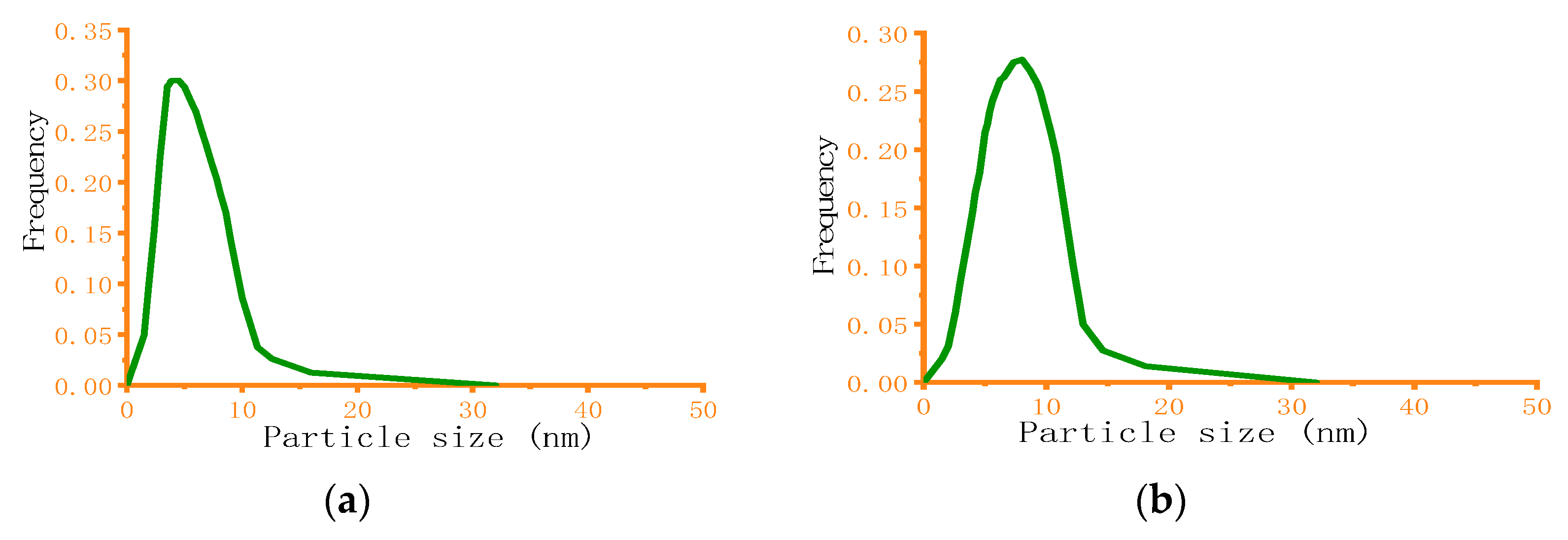
] represents experimental data and solid line [ Crystals 11 00144 i002] represents simulation data).
Crystals 11 00144 g008
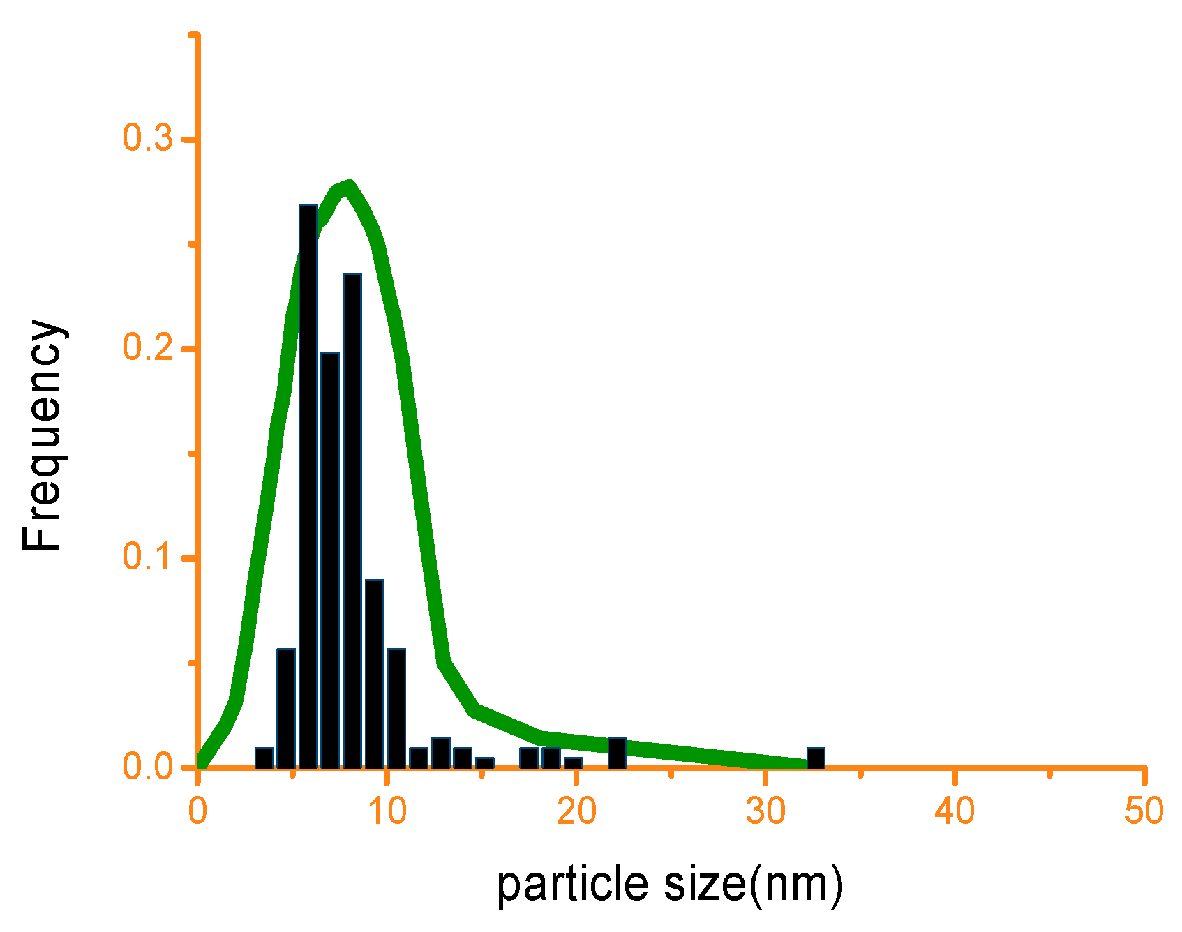
Publisher’s Note: MDPI stays neutral with regard to jurisdictional claims in published maps and institutional affiliations.

