Modeling Hardness Evolution during the Post-Welding Heat Treatment of a Friction Stir Welded 2050-T34 Alloy

Abstract

A unified constitutive model of yield strength evolution during heat treatment has been revised to simulate the hardness evolution during the post-welding heat treatment of AA2050-T34 Friction Stir Welded (FSW) plates. The model considers the strengthening by dislocations, solid solution, clusters, and the T₁ phase. As a result, the successful prediction of yield strength evolution during the aging of AA2050 with different initial tempers has been achieved. The kinetics of precipitation of the T₁ phase during heat treatment has been characterized by electrical resistivity on the unwelded and FSW samples. The obtained results have been used to check the ability of the model to simulate the evolution of the relative volume fraction of the T₁ phase and hardness during the post-welding heat treatment in the different zones of FSW samples. Despite some observed discrepancies on the top and bottom of the weld joint, the revised numerical model captures well the overall hardness profile after the post-weld heat treatment.

1. Introduction

Friction Stir Welding (FSW) is a solid-state joining process invented in 1991 which is known to create a defect-free welding of aluminum alloys [1]. This process induces two effects on the material, the first one is the heat engendered by the friction of the tool and the shoulder on the material. The second one is the plastic strain generated by the stir in the nugget and the thermo-mechanically affected zone (TMAZ). In heat-treated aluminum alloys, this leads to a heterogeneous weld joint with different fractions of precipitates and different levels of mechanical properties between the heat-affected zone (HAZ), TMAZ, and nugget zone. The shape of these different zones, the nugget grain size, the dislocation density, and the heterogeneity of precipitate distribution will greatly depend on welding parameters (travel speed, rotational speed, etc.) as well as the geometry of the tool [2,3].

AA2050 is an Al-Cu-Li-based alloy that has been developed recently for its low density, high strength, and good corrosion resistance, making it valuable for aerospace applications. These remarkable properties are mainly due to the precipitation of the T₁ phase (Al₂CuLi) [4,5,6,7]. At the T34 metallurgical state, where the material has been solution treated, stretched by 3.5%, and naturally aged, the volume fraction of the T₁ precipitate is negligible. To improve its mechanical properties, the alloy must be heat treated for 30 h at 155 °C to reach the T8 state. The yield strength or hardness evolution during this heat treatment has been studied by multiple authors [6,8,9] and the simulation of these evolutions for AA 2050-T34 has also been performed in the literature [9].

Several authors have studied the effect of FSW on AA 2050-T34 [5,6,10]. After welding, homogeneous mechanical properties have been observed in the weld joint [5,6]. Only a small drop of hardness can be observed in the HAZ due to the reversion of clusters. If a post-welding heat treatment at 155 °C for 30 h is performed on the weld joint, the hardness level is raised in the base material and the HAZ until it reaches the hardness of the material at the T8 state. However, a low hardness level is found in the nugget zone. Multiple authors [5,6,10] ascribe this phenomenon to a low precipitation of the T₁ phase due to recrystallization in the nugget caused by a high temperature and high deformation level, leading to low dislocation density in this area. Moreover, different hardness levels between the top and the bottom of the weld joint have also been observed [6,10]. According to [6], this could be due to the presence of different fractions of Cu-containing intermetallic particles which will limit the precipitation of the T₁ phase. Predicting these hardness evolutions after the post-welding heat treatment of FSW plates is thus not only of scientific interest but also of great practical importance to the aerospace industry. However, to the best of the author’s knowledge, no model enabling this prediction is available in the literature.

In this paper, a unified constitutive model of yield strength evolution during heat treatment has been revisited to simulate the post-welding heat treatment of FSW plates. First, characterization by electrical resistivity has been performed on the unwelded material and on FSW samples to follow the kinetics of precipitation of the T₁ phase during heat treatment. Then, using recent microstructural data [11], a revised version of the model of [9] is presented which enables the prediction of yield strength evolution during the aging of AA2050 with different initial tempers, i.e., with different initial volume fractions of clusters, dislocation density, or composition of the solid solution. Finally, the revised model has been used to simulate the evolution of the relative volume fraction of the T₁ phase and hardness during the post-welding heat treatment in the different zones of FSW samples, and a comparison to experimental data is presented.

2. Materials and Methods

The material used in this study is an aluminum-copper-lithium alloy 2050 (Al base, 3.6 wt% Cu, 0.9 wt% Li) provided by Constellium (France). It consisted of 20 mm thick rolled plates at the T34 metallurgical state. After machining, FSW experiments were performed on 15 mm thick plates, the welding direction being parallel to the rolling direction. The welding parameters were chosen to be the same that were used by [6] to be able to rely on their microstructural characterization results. So, a welding speed of 200 mm/min with a rotational speed of 400 rpm under a load of 38 kN was used. The tool was a threaded conical pin with three flat tools and the shoulder was smooth and concave with a tilt angle of 1°.

Welded plates were heat treated in a laboratory oven at 155 °C for 30 h. The welding joint was characterized by microhardness before and after the post-welding heat treatment. Vickers microhardness was measured with a fully automated Struers Durascan hardness tester under a load of 300 g and a dwell time of 10 s. Hardness mapping was realized with a grid spacing of 500 µm in the horizontal and vertical directions on a total width of 70 mm centered on the weld center and a total height of 13 mm.

Precipitation upon heating of the AA2050-T34 samples was characterized by differential scanning calorimetry (DSC) at a heating rate of 20 K/min. A Netzsch 204F1 Phoenix heat flow differential scanning calorimeter was used with cylindrical samples (5 mm diameter, 2 mm thick) placed in standard aluminum crucibles (pierced lid). A high-purity aluminum Al4N reference sample of the same weight as the AA2050-T34 sample was placed in the reference furnace to ensure a similar heat capacity between the sample and reference. Measurements were done at ambient pressure and under nitrogen as a protective gas. The experimental procedure is based on the works of Milkereit et al. [12]. First, an instrumental baseline with Al4N samples in reference and sample furnaces is measured. This instrumental baseline is then subtracted from the heat flow curve of the corresponding sample measurement. This is followed by the subtraction of the experimental baseline determined by a polynomial fit of the background of the resulting curve. The resulting corrected heat flow curve is then normalized by dividing by sample mass and heating rate to obtain the excess specific heat capacity.

Electrical resistivity measurements by classical four-point and multi-point methods were also performed to follow the precipitation of the T₁ phase. Wires in alumel (400 µm diameter for current and 250 µm diameter for tension) and a K-type thermocouple (wire diameter of 250 µm) were embedded in specimens in separate holes with a 650 µm diameter and 600 µm depth. The current through the samples was set to 1A. For each measurement, the high-purity aluminum Al4N resistivity value measured at the same temperature was subtracted from the current resistivity value. Classical four-point resistivity measurements were achieved upon heating the AA2050-T34 of unwelded specimens. The specimen instrumentation is shown in Figure 1a. A multi-point method was also used on the welding joint during the heat treatment at 155 °C. Instead of two wires, 14 wires were used to measure the tension, allowing 13 areas of measurement to be considered simultaneously, see Figure 1b. Specimens were taken transversally to the welding direction and at different heights to characterize the whole weld joint.

The modeling of yield strength and hardness evolution in AA2050 specimens with different initial tempers and FSW welded plates during post-weld heat treatment was achieved with the Python language.

3. Experimental Results

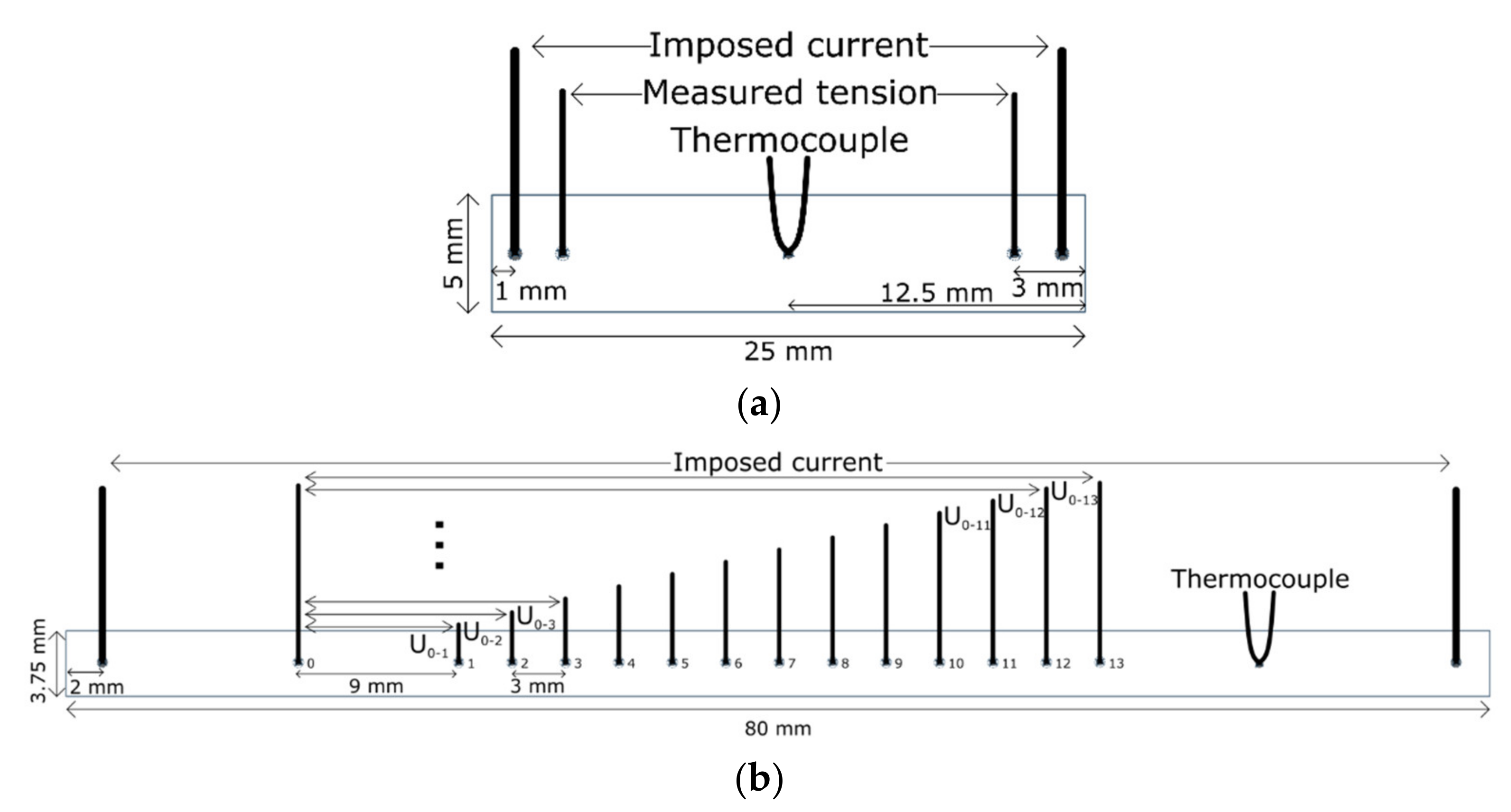
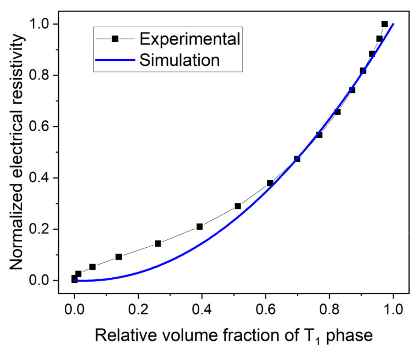
3.1. Monitoring T₁ Precipitate Evolution Using Electrical Resistivity Measurement

An electrical resistivity measurement was performed to characterize the precipitation of the T₁ phase in AA2050-T34 during heat treatment. First, the evolution of electrical resistivity during heating at 20 K/min was compared to the DSC thermogram obtained in the same conditions. In Figure 2, the temperature derivative of electrical resistivity and the excess specific heat capacity was plotted vs. temperature. According to the literature [5,6,10,13,14], peak A observed in the DSC curve is due to the reversion of the clusters, peak B is due to the precipitation of the T₁ phase, and peak C corresponds to the thickening of these precipitates. The precipitation of the θ’ phase can be observed in peak D and finally the dissolution of the T₁ phase results in peak E. The comparison between the two techniques shows that the precipitation of the T₁ phase (peak B on the DSC curve) induces a rise in electrical resistivity. This abnormal evolution is either due to the inherent high resistivity of the T₁ phase according to [15] or to the presence of strain fields around the precipitates that act as electron scattering centers [16,17,18,19].

The methodology proposed by [20] and based on the Matthiessen equation has been used to calculate the evolution of the relative volume fraction of the T₁ phase according to the evolution of electrical resistivity. First, the electrical resistivity is considered to be dominated by the contribution of solutes atoms and precipitates as expressed in Equation (1):

$${\rho }_e={\rho }_{SS}+{\rho }_{PPT}$$

(1)

where ${\rho }_{SS}$ could be determined as the electrical resistivity of the material after solution heat treatment. To consider the abnormal rise of electrical resistivity due to the formation of the T₁ phase, a term related to the resistivity of the T₁ phase was added to the one representative of the depleted solute concentration occurring during precipitation as expressed in Equation (2):

$${\rho }_{PPT}=f_v{}^a{\rho }_{T_1}-f_v\left({\rho }_{Cu}{X}_{Cu}+{\rho }_{Li}{X}_{Li}\right)$$

(2)

where $f_v$ corresponds to the volume fraction of the T₁ phase, $a$ is an exponent, ${\rho }_{T_1}$ is the electrical resistivity of T₁, ${\rho }_{Cu}$ and ${\rho }_{Li}$ are the solute coefficients for Cu and Li atoms in the solid solution, and $X_{Cu}$ and $X_{Li}$ are the Cu and Li atom fractions in the T₁ phase, respectively.

In Equation (1), the minimal and maximal values of ${\rho }_e$ correspond to a solution annealing of a heat-treated sample and a sample with maximal volume fraction of the T₁ phase (i.e., T8 state), respectively. The normalized value of electrical resistivity could then be expressed as Equations (3) and (4):

$${\overline{\rho }}_e=\frac{{\rho }_e-{\rho }_{e_{min}}}{{\rho }_e-{\rho }_{e_{max}}}=\frac{({\rho }_{SS}+{\rho }_{PPT})-{\rho }_{SS}}{({\rho }_{SS}+{\rho }_{PP{T}_{max}})-{\rho }_{SS}}$$

(3)

$${\overline{\rho }}_e=\frac{{\rho }_{PPT}}{{\rho }_{PP{T}_{max}}}=\frac{f_v{}^a{\rho }_{T_1}-f_v\left({\rho }_{Cu}{X}_{Cu}+{\rho }_{Li}{X}_{Li}\right)}{{{f_v}_{max}}^a{\rho }_{T_1}-{f_v}_{max}\left({\rho }_{Cu}{X}_{Cu}+{\rho }_{Li}{X}_{Li}\right)}$$

(4)

where ${f_v}_{max}$ is the volume fraction of the T₁ phase at the T8 state taken as 3.79% [11].

The normalized value of electrical resistivity could be then related to the relative volume fraction of the T₁ phase $\overline{f_v}=f_v/{f_v}_{max}$ through Equation (5):

$${\overline{\rho }}_e=\frac{{{f_v}_{max}}^a{\rho }_{T_1}}{{{f_v}_{max}}^a{\rho }_{T_1}-{f_v}_{max}\left({\rho }_{Cu}{X}_{Cu}+{\rho }_{Li}{X}_{Li}\right)}{\overline{f_v}}^a-\frac{{f_v}_{max}\left({\rho }_{Cu}{X}_{Cu}+{\rho }_{Li}{X}_{Li}\right)}{{{f_v}_{max}}^a{\rho }_{T_1}-{f_v}_{max}\left({\rho }_{Cu}{X}_{Cu}+{\rho }_{Li}{X}_{Li}\right)}\overline{f_v}$$

(5)

According to the literature, a value of 8 × 10⁻⁹ Ω.m for ${\rho }_{Cu}$ [21] and 9.9 × 10⁻⁹ Ω.m for ${\rho }_{Li}$ [22] were used. The exponent $a$ takes the value of 2 and ${\rho }_{T_1}$ has been set to 2 × 10⁻⁸ Ω.m to fit experimental data leading to Equation (6):

$${\overline{\rho }}_e=1.063\times {\overline{f_v}}^2-0.063\times \overline{f_v}$$

(6)

Figure 3 shows the evolution of normalized electrical resistivity vs. the relative volume fraction of the T₁ phase measured by DSC. A comparison between experimental measurements and simulated ones by Equation (6) shows some discrepancies that can be observed at a low relative volume fraction of the T₁ phase but the simulation is close to experimental data for the relative volume fraction of the T₁ phase above 0.5. It is worth mentioning that the effects of the size, shape, and orientation of the plate-like T₁ precipitates on the electrical resistivity measurements were not specifically studied in this work. Such a study could help to address the issue of the observed differences, especially at a low relative volume fraction of the T₁ phase.

3.2. Kinetics of Precipitation of the T₁ Phase during Post-Welding Heat Treatment

Keeping in mind this overestimation of the low values of relative volume fraction, an electrical resistivity measurement with a multi-point method was used to characterize the precipitation of the T₁ phase during heat treatment at 155 °C for 30 h in the weld joint. Equation (6) is then used to characterize the evolution of the relative volume fraction of the T₁ phase and the data are compared to the small angle X-ray scattering (SAXS) measurements performed by [6] as shown in Figure 4a–c. Three distances from the weld center (Figure 4d) are presented (± 13.5, 7.5, and 1.5 mm) with measurements close to the top surface (z = 13 mm against 13.5 mm in [6]) and close to the bottom surface (z = 1.5 mm against 2 mm in [6]). The first decrease in electrical resistivity after one hour of heat treatment is probably due to the reversion of clusters. So, the value of the relative fraction calculated in this domain is not relevant and will not be discussed here. After one hour of heat treatment, it is clear in Figure 4 that the kinetics of precipitation at the top of the weld measured by electrical resistivity is close to those determined by SAXS measurements [6]. Some discrepancies can be observed for the bottom of the weld and especially at the end of the heat treatment. Indeed, close to the center (1.5 mm), the relative volume fraction of the T₁ phase obtained by electrical resistivity after 30 h of heat treatment is close to 0.5, where the value measured by [6] was close to 0.2.

Multi-point electrical resistivity also allows for mapping the relative volume fraction of the T₁ phase after 30 h of post-welding heat treatment at 155 °C. Obtained values from 10 of the 13 areas of measurement on the bottom, top, and mid-lines of the weld joint are marked in Figure 5a. Furthermore, in Figure 5b, hardness isovalue curves measured after the heat treatment were superimposed on the map of the relative volume fraction of the T₁ phase. The low hardness level measured in the weld nugget is clearly superimposed with the low volume fraction of precipitates measured by electrical resistivity, which means that the size of the soften zone is properly determined by electrical resistivity. However, as observed previously, the relative volume fraction of the T₁ phase obtained by electrical resistivity in the bottom center of the weld joint seems to be overestimated and is too high compared to the hardness level measured.

4. Modeling

4.1. Original Constitutive Model

The unified constitutive model developed by Li [9] for the artificial aging of AA2050 was used in this study. This model can simultaneously predict the evolutions of microstructures and yield strength during the aging of AA2050-T34 at 155 °C by taking into account the strengthening by dislocations, solid solution, clusters, and T₁ precipitates. The set of the corresponding constitutive equations is first given in this section.

4.1.1. Dislocations

The evolution of normalized dislocation density during artificial aging due to the recovery is calculated with Equation (7):

$$\dot{\overline{\rho } }=-C_p{\overline{\rho }}^{m_4}$$

(7)

where $C_p$ and $m_4$ are material constants characterizing the recovery process, and $\overline{\rho }$ is the normalized dislocation density which is calculated with Equation (8):

$$\overline{\rho }=\left(\rho -{\rho }_i\right)/{\rho }_s$$

(8)

where ${\rho }_i$ is the dislocation density after solution heat treatment and ${\rho }_s$ is the dislocation density at the T34 state. The hardening due to the dislocation density is then calculated with Equation (9) using Kocks’ law [23]:

$${\sigma }_{dis}= A_3{\overline{\rho }}^{0.5}$$

(9)

where $A_3$ is a constant.

4.1.2. Solid Solution

The solute concentration will evolve during artificial aging due to the dissolution of the clusters and the precipitation of the T₁ phase. As previous authors have pointed out [24], the dislocation density contributes to the precipitation of the T₁ phase and enhances the kinetics of precipitation. The rate evolution of the normalized solute concentration is calculated with Equation (10):

$$\dot{\overline{c}}=-A_1\left(\overline{c}-{\overline{c}}_a\right)\left(1+{\gamma }_0{\overline{\rho }}^{m_2}\right)+A_2{\overline{r}}_d$$

(10)

where $A_1$, ${\gamma }_0$, and $m_2$ are constants. $\overline{c}$ is the normalized solute concentration defined as $c/c_s$ with $c$ as the solute concentration and $c_s$ as the solute concentration after solution heat treatment. ${\overline{c}}_a$ is defined as $c_a/c_s$ with $c_a$ as the equilibrium solute concentration at the temperature of artificial aging (155 °C). Hardening from the solid solution is then calculated with Equation (11) [25]:

$${\sigma }_{ss}= C_{ss}{\overline{c}}^{\frac{2}{3}}$$

(11)

4.1.3. Clusters

The dissolution of Cu-rich clusters at the beginning of the artificial aging is modeled by the evolution of the normalized cluster radius ${\overline{r}}_d$ in Equation (12):

$${\dot{\overline{r}}}_d=-\frac{C_{r1}}{{\overline{r}}_d}$$

(12)

where $C_{r1}$ is a constant. Clusters here are considered small and shearable, according to [9]. For that reason, Equation (13), for the shearing of precipitates presented by [25], was taken for the hardening due to the presence of clusters:

$${\sigma }_{p-d}= C_{a1}{\overline{r}}_d^2$$

(13)

4.1.4. T₁ Precipitates

For the T₁ phase, which is the hardening phase in the material, the evolution of the normalized precipitate radius and the normalized thickness during artificial aging is calculated with Equations (14) and (15):

$${\dot{\overline{r}}}_n= C_r{\left(Q-{\overline{r}}_n\right)}^{m_1}\left(1+{\gamma }_0{\overline{\rho }}^{m_2}\right)$$

(14)

$$\left\{\begin{array}{c}\dot{\overline{h}}=0 \left({\overline{r}}_n<1\right)\\ \dot{\overline{h}}= \frac{1}{3}\frac{\beta D}{\overline{h}}= \frac{C_h}{\overline{h}} \left({\overline{r}}_n\ge 1\right)\end{array}\right.$$

(15)

where $C_r$, $C_h$, and $m_4$ are constants. ${\overline{r}}_n$ is the normalized precipitate radius defined as $r_n/r_c$ with $r_c$ as the critical radius at the peak aging state and $Q$ as the saturated value of ${\overline{r}}_n$ during artificial aging.$\overline{h}$ is the normalized thickness of the precipitate defined as $h/h_c$ with $h_c$ as the critical thickness [9]. The thickness of the precipitates will only rise when the peak aging has been reached. The thickening of the T₁ phase will allow the transition between shearing and bypassing strengthening mechanisms.

The normalized volume fraction of the T₁ phase is calculated with Equation (16) using the solute concentration of the material and the normalized fraction of clusters:

$${\overline{f}}_n=\frac{1-\overline{c}}{1-{\overline{c}}_a}-{\overline{f}}_d$$

(16)

In order to take into account the shearing and bypassing strengthening mechanisms, it was chosen by [9] in Equation (17) to calculate the harmonic mean of the two equations to determine the hardening due to the precipitation of the T₁ phase during artificial aging:

$${\sigma }_{p-n}=\frac{{\sigma }_{shear}{\sigma }_{bypass}}{{\sigma }_{shearé}+{\sigma }_{bypass}}= {\sigma }_r\frac{{\overline{f}}_n^{m_5}}{{\overline{h}}^{m_6}}$$

(17)

where $m_5$ and $m_6$ are constants and ${\sigma }_r$ represents the strengthening effect from the precipitate radius calculated by Equation (18):

$${\dot{\sigma }}_r= C_a{\dot{\overline{r}}}_n^{m_7}\left(1-{\overline{r}}_n^{m_8}\right)$$

(18)

where $C_a$, $m_7$, and $m_8$ are constants.

4.1.5. Yield Strength

The overall hardening from precipitate is then calculated by Equation (19) with a classical law of mixture which considers the dissolving clusters and the precipitation of the T₁ phase:

$${\sigma }_p= \sqrt{{\sigma }_{p-d}^2+{\sigma }_{p-n}^2}$$

(19)

Finally, the overall yield strength is calculated with the contribution of dislocations, solid solution, and the precipitates as expressed in Equation (20):

$${\sigma }_y={\sigma }_{ss}+{\left({\sigma }_{dis}^N+{\sigma }_p^N\right)}^{\frac{1}{N}}$$

(20)

where $N$ is a parameter representing the transition of the precipitates from shearable to non-shearable which varies from 1 to 2 according to the thickness of the precipitates.

4.1.6. Summary and Material Constants

The unified constitutive model is summarized in

Table 1. Summary of the equations of the original model [9].

Dislocations	Solid Solution	Clusters
$\dot{\overline{\rho } }=-C_p{\overline{\rho }}^{m_4}$	$\dot{\overline{c}}=-A_1\left(\overline{c}-{\overline{c}}_a\right)\left(1+{\gamma }_0{\overline{\rho }}^{m_2}\right)+A_2{\overline{r}}_d$	${\dot{\overline{r}}}_d=-\frac{C_{r1}}{{\overline{r}}_d}$
${\sigma }_{dis}= A_3{\overline{\rho }}^{0.5}$	${\sigma }_{ss}= C_{ss}{\overline{c}}^{2/3}$	${\overline{f}}_d= {\overline{f}}_{d_0}{\left(\frac{{\overline{r}}_d}{{\overline{r}}_{d_0}}\right)}^3$
		${\sigma }_{p-d}= C_{a1}{\overline{r}}_d^2$
Precipitates	Yield Strength
${\dot{\overline{r}}}_n= C_r{\left(Q-{\overline{r}}_n\right)}^{m_1}\left(1+{\gamma }_0{\overline{\rho }}^{m_2}\right)$	${\sigma }_p= \sqrt{{\sigma }_{p-d}^2+{\sigma }_{p-n}^2}$
$\left\{\begin{array}{c}\dot{\overline{h}}=0 \left({\overline{r}}_n<1\right)\\ \dot{\overline{h}}= \frac{C_h}{\overline{h}} \left({\overline{r}}_n\ge 1\right)\end{array}\right.$	${\sigma }_y={\sigma }_{ss}+{\left({\sigma }_{dis}^N+{\sigma }_p^N\right)}^{\frac{1}{N}}$
$\overline{f}= {\overline{f}}_d+{\overline{f}}_n=\frac{1-\overline{c}}{1-{\overline{c}}_a}$
${\sigma }_{p-n}= {\sigma }_r\frac{{\overline{f}}_n^{m_5}}{{\overline{h}}^{m_6}}$
${\dot{\sigma }}_r= C_a{\dot{\overline{r}}}_n^{m_7}\left(1-{\overline{r}}_n^{m_8}\right)$

. The values of material constants used in the model for the artificial aging of AA2050-T34 [9] are presented in

Table 2. Summary of material constants used in the model for the artificial aging of AA2050-T34. Data from [9].

Parameter	Value	Parameter	Value	Parameter	Value
$C_p \left({\mathrm{h}}^{-1}\right)$	0.1	$A_2 \left({\mathrm{h}}^{-1}\right)$	0.045	$C_h$	8 × 10−5
$m_4$	6.5	$C_{ss} \left(\mathrm{MPa}\right)$	120	$m_5$	0.3
$A_3 \left(\mathrm{MPa}\right)$	100	$C_{r1 }\left({\mathrm{h}}^{-1}\right)$	0.185	$m_6$	0.05
$A_{1 }\left({\mathrm{h}}^{-1}\right)$	0.05	$C_{a1} \left(\mathrm{MPa}\right)$	52	$C_a \left(\mathrm{MPa}\right)$	36.3
${\overline{c}}_a$	0.316	$C_{r }\left({\mathrm{h}}^{-1}\right)$	0.238	$m_7$	0.06
$m_2$	1.28	$Q$	1	$m_8$	9.5
${\gamma }_0$	0.08	$m_1$	1.05	$A_4$	0.22

.

4.1.7. Comparison to Experimental Values

The comparison between the result of the simulation with the model described above and measurements from different authors [6,9,26] for the heat treatment of AA2050-T34 presents a good agreement (Figure 6). The relationship between yield strength and hardness for AA2050 is based on the results of [9] and given by Equation (21):

$${\sigma }_y=-185.1+3.795\ast HV$$

(21)

4.2. Revised Version of the Model

A revised version of the model is presented which enables the prediction of yield strength evolution during the aging of AA2050 with different initial tempers.

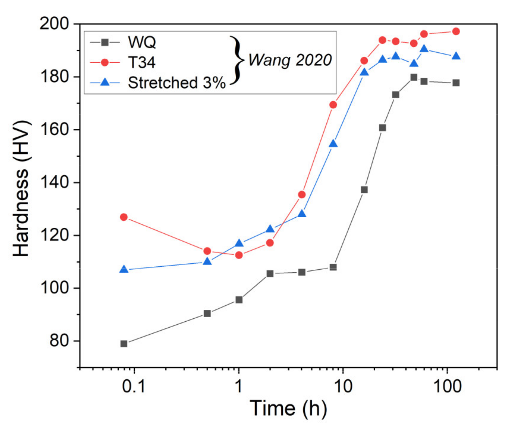
4.2.1. Influence of Pre-Treatments

In recent work, Wang et al. [11] studied the influence of pre-treatments on the microstructure of Al-Li-Cu alloy with a chemical composition close to the alloy studied in this work. The behavior during artificial aging at 155 °C of the same alloy with different initial states, called here “WQ”, “Stretched 3%”, and “T34”, was studied. The “WQ” case corresponds to a sample first solution heat-treated and then water-quenched. “Stretched 3%” corresponds to a sample “WQ” subsequently stretched by 3%. Finally, the “T34” state is the sample stretched 3% and then naturally aged at room temperature. The evolutions of the hardness of the Stretched 3% and the T34 samples are quite similar, with a slight difference at the beginning of artificial aging due to the reversion of clusters (Figure 7). For the WQ state, the hardness evolution is quite different with a lower hardness level and an increase in hardness slower than in the T34 case. These effects are mainly due to the low dislocation density in the material at the WQ state as pointed out by the literature [5,6,10]. The authors determined the evolution of the radius of the T₁ precipitates during heat treatment by HAADF-STEM. The evolution of the volume fraction of the T₁ phase has also been characterized by differential scanning calorimetry and SAXS. It was observed that a high dislocation density and natural aging promote the formation of the T₁ phase. In contrast, the absence of pre-stretching and natural aging hinders the formation of the T₁ phase and promotes the formation of other phases such as θ’. Furthermore, a low volume fraction of the T₁ phase leads to a high radius of the precipitates and thus to low hardening.

4.2.2. Simulations with the Original Model

The model previously presented has been used to simulate the heat treatment at 155 °C in samples with three different pre-treatments. To this end, different initial values of microstructural variables in the model were used (see

Table 3. Initial values of microstructural variables according to different pre-treatments.

Normalized Variable	T34	Stretched 3%	WQ
Cluster radius ${\overline{r}}_{d_0}$	1	0	0
Cluster volume fraction ${\overline{f}}_{d_0}$	0.032	0	0
Dislocation density ${\overline{\rho }}_0$	1	1	0
Solid solution concentration ${\overline{C}}_0$	0.978	1	1

).

Results obtained by this method clearly show a superposition of the evolution of the radius and volume fraction of the T₁ phase for the three cases (Figure 8).

The evolution of the normalized radius in the T34 state is very well predicted by the model of Li since it has been previously calibrated by the author with experimental data [4,8,27]. However, this is not the case for the WQ and Stretched 3% states. Moreover, the evolution of the normalized volume fraction of T₁ in the T34 state was not properly simulated. This means that it is necessary to revise the model to better take into account the evolution of the normalized volume fractions while increasing the effect of dislocation density on the kinetics of precipitation.

4.2.3. Revised Model

Modifications of the original model have been carried out on the simulation of the normalized volume fraction, the normalized radius, and the strength contribution of the T₁ precipitates. The calibration of the model has been performed on the data of [11] according to the initial state of the material.

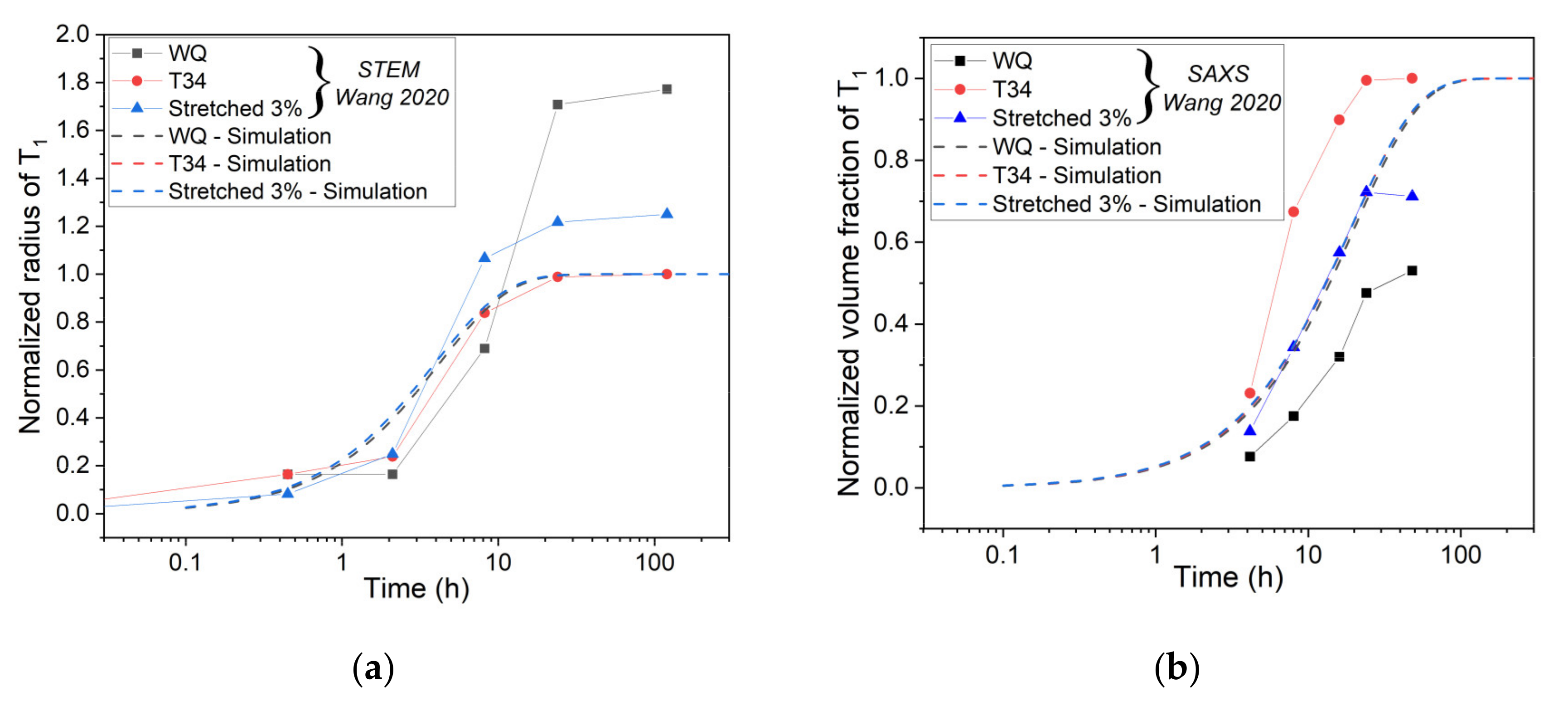
Normalized Volume Fraction of the T₁ Phase

To begin, the focus was on the evolution of the relative fraction of the T₁ phase. As observed by [11], the reduction in the dislocation density and volume fraction of clusters promotes the precipitation of other phases such as the θ’ phase which is considered here as a non-hardening phase. The precipitation of these phases limits the precipitation of the T₁ phase due to fewer elements in the solid solution. Therefore, Equation (16) was modified into Equation (21) which considers the formation of other phases such as the θ’ phase to limit the maximal volume fraction of the T₁ phase.

$$\overline{f}= {\overline{f}}_d+{\overline{f}}_n+{\overline{f}}_t=\frac{1-\overline{c}}{1-{\overline{c}}_a}$$

(22)

where ${\overline{f}}_t$ is the normalized precipitate fraction of non-hardening phases such as the θ’ phase. To be consistent with the rate evolution of Equation (10) for a solid solution, the evolution of ${\overline{f}}_t$ is controlled by the rate evolution of Equation (22):

$$\dot{{\overline{f}}_t}= A_1\left({\overline{f}}_{tm}-{\overline{f}}_t\right)\left(1+{\gamma }_0{\overline{\rho }}^{m_2}\right)$$

(23)

where ${\overline{f}}_{tm}$ corresponds to the maximum normalized volume fraction of the non-hardening phase. This variable will take the value of 0 for the T34, 0.19 for the Stretched 3%, and 0.47 for the WQ states, respectively.

Finally, the effect of dislocation density on the kinetics of precipitation has been increased by an augmentation of the value of ${\gamma }_0$ (Equation (10)) from 0.08 to 1.7. The result of the two modifications can be observed in Figure 9. The modified version of the model predicts very well the kinetics of precipitation and the maximal normalized volume fraction of the T₁ phase for the three cases presented.

Normalized Radius of the T₁ Precipitates

For a second time, the evolution of the normalized radius of the T₁ precipitate during artificial aging has been studied. As observed by [11,28], the high-volume fraction of the T₁ phase after 30 h of heat treatment leads to a low radius of precipitates. On the opposite, a low volume fraction of the T₁ phase after the heat treatment leads to a higher average radius of the precipitates. To take this phenomenon into account, the value of Q (Equation (14)) now depends on the maximal normalized volume fraction that can be formed during artificial aging. The form of the equation and the value of the parameters was chosen to best fit the experimental data obtained with different initial states (Figure 10a).

$$Q=4.69-7.52\times {{\overline{f}}_n}_{max}+3.83\times {{{\overline{f}}_n}_{max}}^2$$

(24)

where ${{\overline{f}}_n}_{max}$ is the maximal volume fraction of the T₁ phase that can be formed during artificial aging at 155 °C.

The value of ${\gamma }_0$ given previously has been kept, meaning that the value of $C_r$ (Equation (14)) must be decreased from 0.238 to 0.079 to be consistent with the T34 state. The results obtained with the modified version of the model can be seen in Figure 10b. The maximal values and rate evolution of the normalized radius of precipitates are well predicted by the simulation.

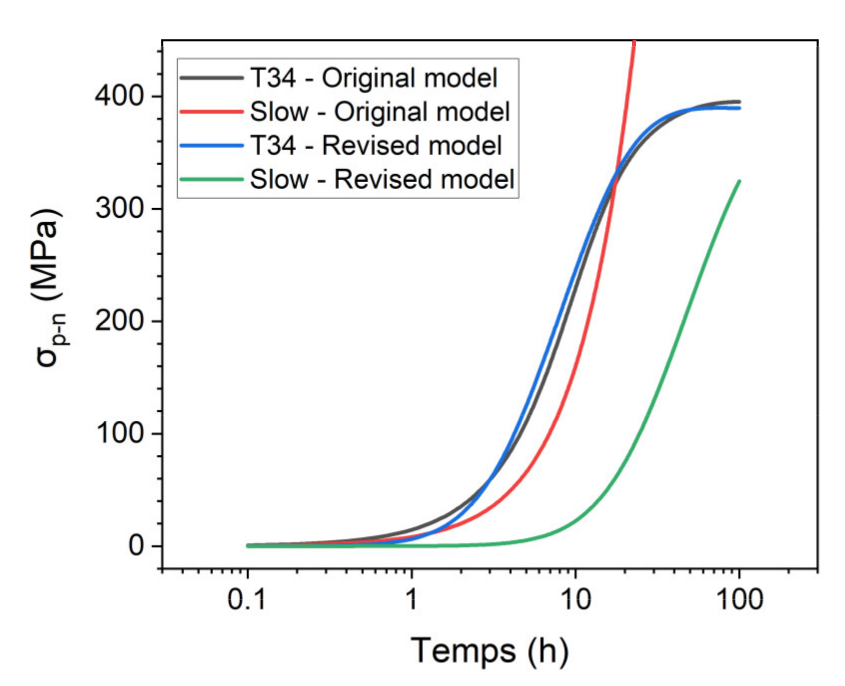
Strength Contribution of the T₁ Precipitates

The modification of the kinetics of precipitation has led to a problem concerning the calculation of ${\sigma }_r$ (Equation (18)). As shown in Figure 11, if the kinetics of precipitation is arbitrarily set five times slower, the calculated strength contribution of the T₁ precipitates ${\sigma }_{p-n}$ exhibits only a minor change at the early stage. However, the evolution of the precipitate radius is still slower, and the maximal radius will be reached five times later. This led to a clear overestimation of the value of ${\sigma }_r$ after 10 h of heat treatment.

To address this difficulty, the equation presented by Li et al. [29] before the mathematical transformation realized by this author is used to calculate the evolution of ${\sigma }_r$ (Equation (25)). The values of the exponent and $C_a$ (700 MPa) were chosen to simulate the same evolution of ${\sigma }_r$ as Li et al. [9] for the T34 state.

$${\sigma }_r=C_a\frac{r_n^2}{r_n^2+1}$$

(25)

As the evolution of the normalized volume fraction of the T₁ phase for the T34 state has been modified to match the experimental data, it was necessary to increase the value of $m_5$ (Equation (17)) to 0.7 to be consistent with the simulation performed by the authors [9]. The simulation for the case with a kinetics of precipitation five times slower then shows only a time offset that validates the modification done here (Figure 11).

The comparison between the hardness evolutions measured by Wang et al. [11] and the simulations achieved with the revised model is presented in Figure 12.

The $C_a$ value was slightly changed to 800 MPa in order to better simulate the highest hardness value observed by the authors. It can be observed that the model may accurately simulate the evolution of hardness during artificial aging for different initial pretreatments. The T34 and Stretched 3% simulated samples present a similar evolution of hardness during the precipitation of the T₁ phase with only a difference at the beginning of the heat treatment due to the presence of clusters in the T34 state. For the WQ state, the rise of hardness is very well depicted with only a small underestimation of the maximal hardness. At the beginning of artificial aging, the experimentally observed rise of hardness is not simulated because the model does not consider the formation of clusters. This is not a problem in this work, since the formation of clusters is not expected during the post-welding heat treatment of AA2050 in the T34 FSW samples [6].

The modified material constants and equations in the revised model are summarized in

Table 4. Material constants and equations modified in the revised model [9,11].

Parameter	Value	Equation
$A_2\left({\mathrm{h}}^{-1}\right)$	$0.012 {\mathrm{h}}^{-1}$	$Q=4.69-7.52\times {{\overline{f}}_n}_{max}+3.83\times {{{\overline{f}}_n}_{max}}^2$
$C_a$	$700 \mathrm{MPa}$ $800 \mathrm{MPa}$	$\frac{1-\overline{c}}{1-{\overline{c}}_a}={\overline{f}}_d+{\overline{f}}_n+{\overline{f}}_t$
$m_5$	0.7	$\dot{{\overline{f}}_t}=A_1\left({\overline{f}}_{tm}-{\overline{f}}_t\right)\left(1+{\gamma }_0{\overline{\rho }}^{m_2}\right)$
${\overline{f}}_{tm}-T34$	0	${\sigma }_r=C_a\frac{r_n^2}{r_n^2+1}$
${\overline{f}}_{tm}-Stretched 3\%$	0.19
${\overline{f}}_{tm}-WQ$	0.47
$C_r\left({\mathrm{h}}^{-1}\right)$	0.079
${\gamma }_0$	1.7

.

5. Application to FSW

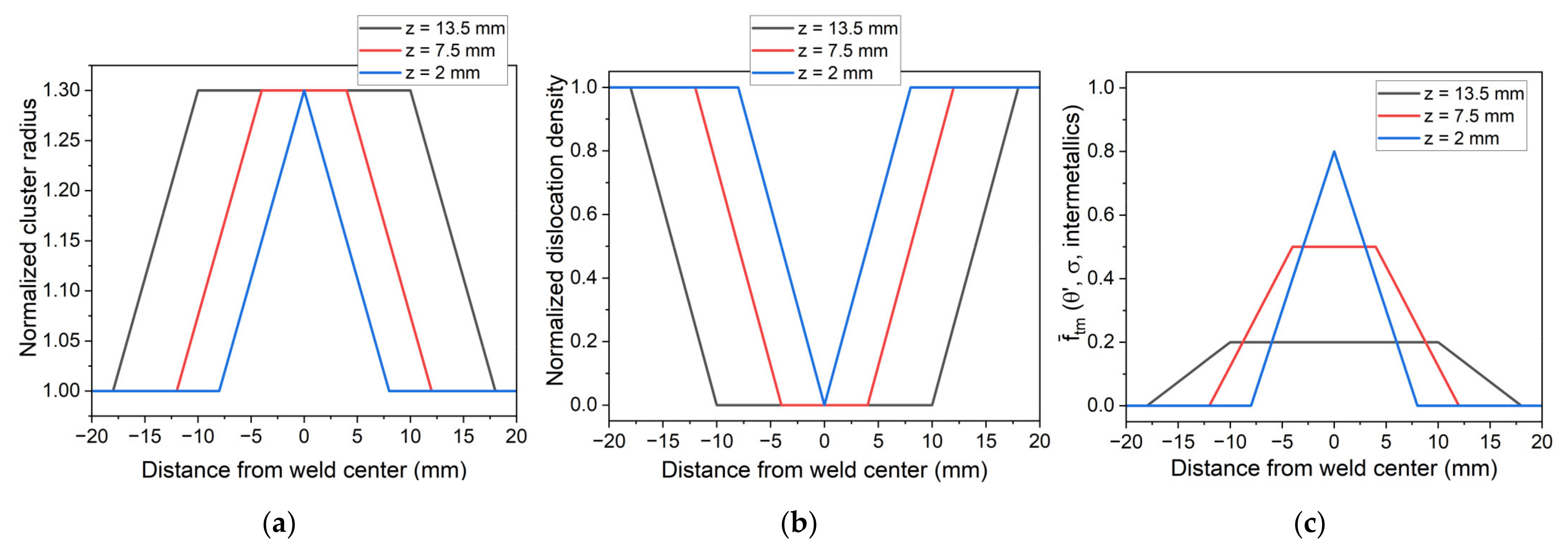
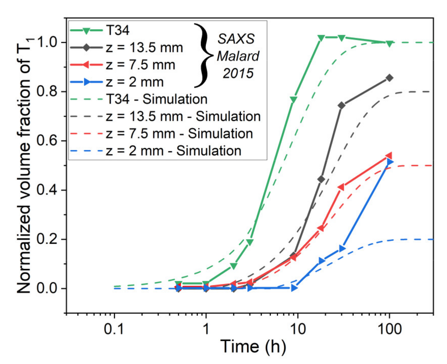
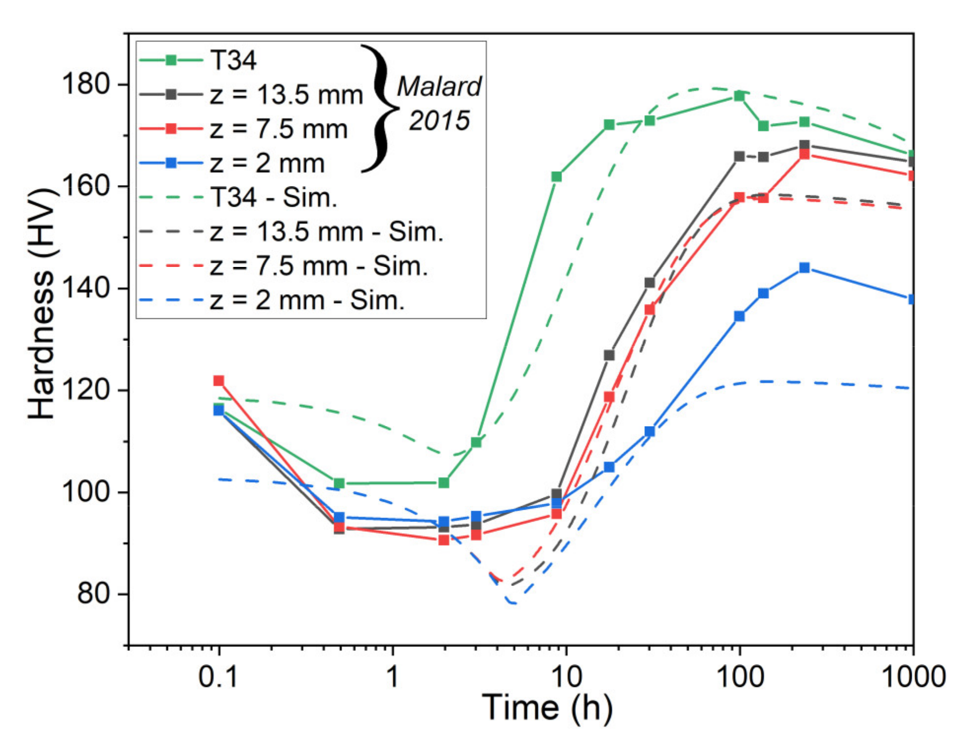
5.1. Simulation of Post-Weld Heat Treatment by Using the SAXS Data from [6]

The revised model was applied to simulate the post-weld heat treatment of FSW plates. To be able to use this model, it was necessary to set the initial state of the material at each location of the weld joint. Since the hardness in the base material and the HAZ reached the hardness of the T8 state after the heat treatment, the T34 state was imposed as the initial state in these zones. The size of the weld nugget was defined first according to the SAXS measurements of [6] after 30 h of heat treatment. The recrystallization that occurred in the weld nugget led to low dislocation density and a slower kinetics of precipitation. So, the normalized volume fraction of the T₁ phase is lower than 1 in the weld nugget. In this area, the normalized radius of the clusters was set to 1.3 to be consistent with the data of [6] (Figure 13a). Due to the recrystallization that occurs in the weld nugget, the normalized dislocation density was set to 0 in this area (Figure 13b) which corresponds to the value used for the WQ state presented before. This value is questionable since the levels of deformation and temperature vary from the top to bottom of the weld joint. However, in absence of a quantitative measurement, this hypothesis was chosen to simulate the weld nugget behavior. Finally, it was necessary to set the maximum normalized volume fraction of non-hardening phases such as θ’ in order to properly simulate the maximum volume fraction of the T₁ phase observed by [6] (Figure 13c).

The evolution of the normalized volume fraction of T₁ phases during the heat treatment simulated by the model is compared to the data of [6] in Figure 14.

The kinetics of precipitation in the nugget at the weld center simulated by the model for the top (z = 13.5 mm) and middle line (z = 7.5 mm) is close to the experimental measurements of [6]. For the bottom line (z = 2 mm), the simulation is close until 30 h of heat treatment but underestimates the relative volume fraction of the T₁ phase after 100 h. However, as explained by [6], the SAXS measurement cannot distinguish the T₁ from θ’ platelets which could lead to an overestimation of the experimental volume fraction of the T₁ phase in this area.

The simulation of the evolution of hardness during heat treatment was also compared to the measurements of [6]. The hardness in the weld nugget at the weld center after 30 h of heat treatment is close to the experimental data (Figure 15). However, the hardness level at a short and long-time is underestimated by the model. This could be due to the value of the normalized dislocation density which was set to 0. For example, an increase to 0.1 will lead to a rise of almost 10 HV with a minor change in the kinetics of precipitation. A more realistic value of normalized dislocation density into the nugget may thus reduce the difference between the experimental and simulated hardness.

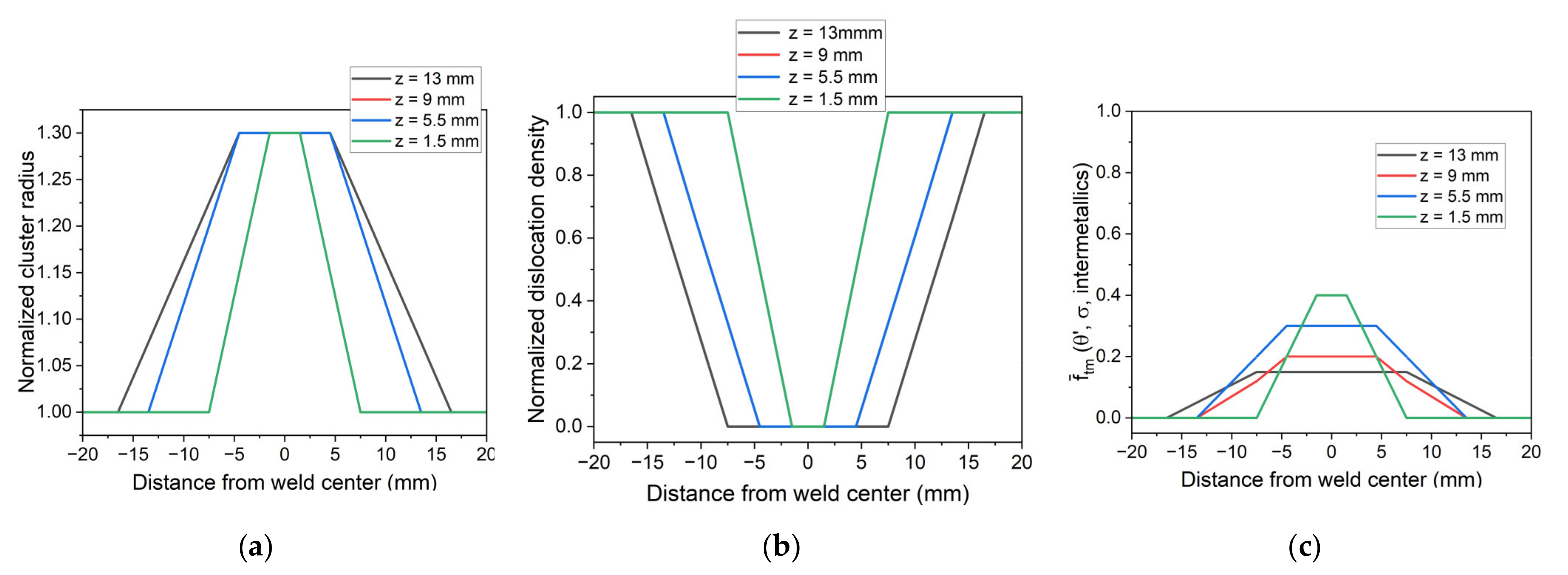
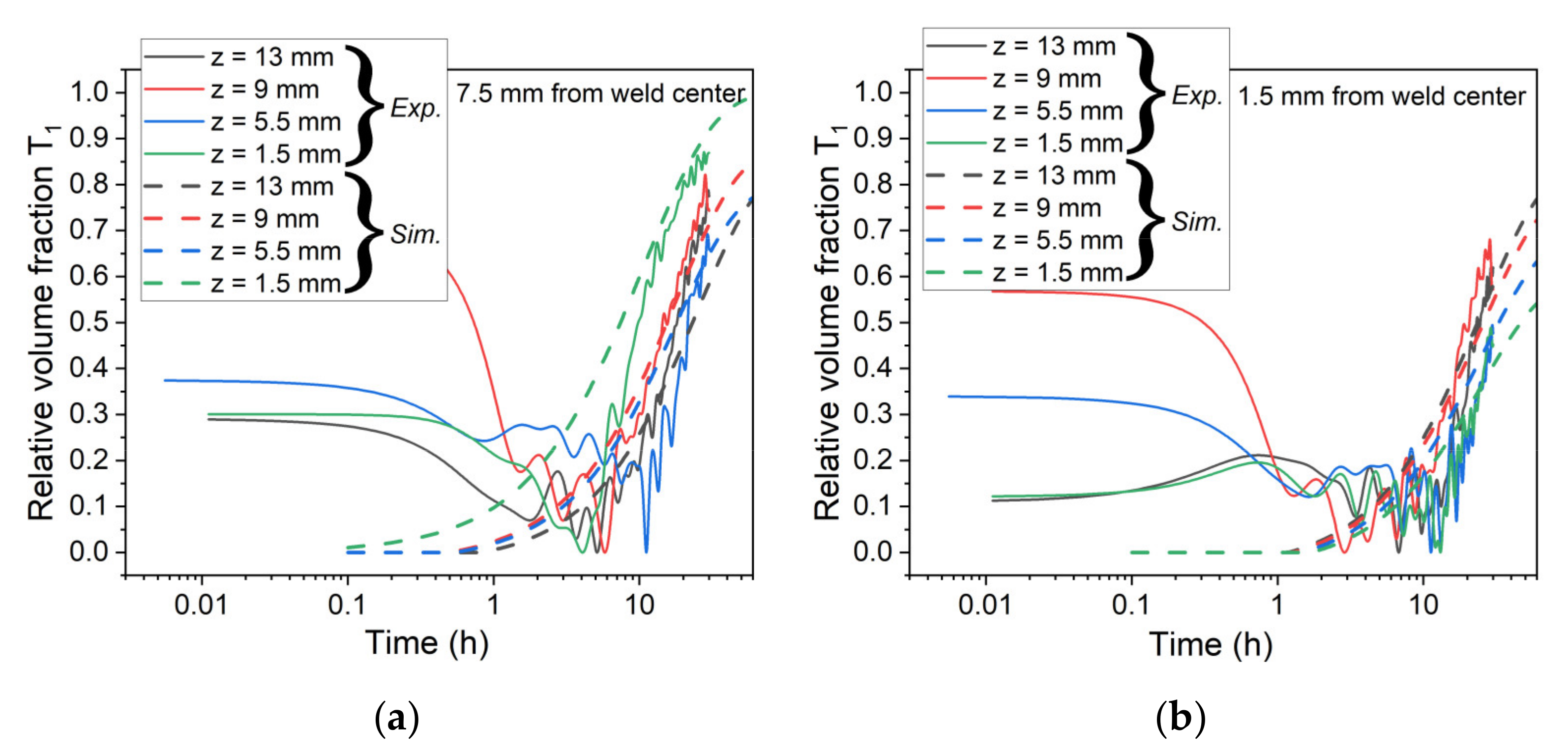
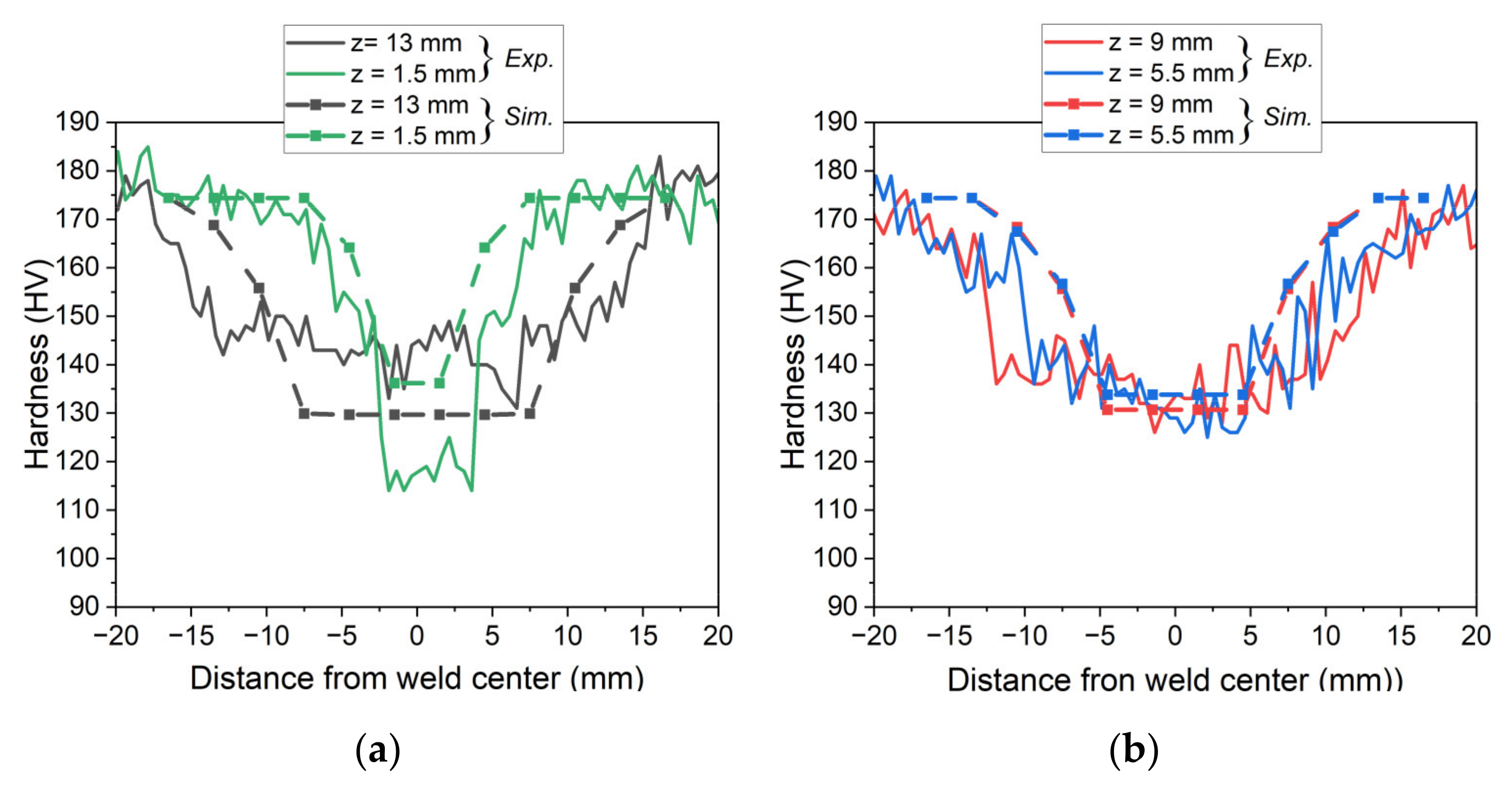
5.2. Simulation of Post-Weld Heat Treatment by Using Electrical Resistivity

The revised model has also been used to simulate the hardness of the weld joint by using electrical resistivity measurements. In the same way as above, the size of the weld nugget and the maximum normalized volume fraction of the non-hardening phases observed at the end of the heat treatment were set according to the normalized volume fraction of the T₁ precipitates measured by electrical resistivity (Figure 16). The normalized radius of the clusters and normalized dislocation density in the weld nugget was set to 1.3 and 0, respectively.

For the sake of simplicity, only the evolution of the relative volume fraction of T₁ at 7.5 and 1.5 mm from the weld center is presented here. The evolution of the relative volume fraction of the T₁ phase simulated by the model shows a good agreement with experimental data obtained from electrical resistivity measurements (Figure 17).

At 7.5 mm from the weld center, the bottom of the weld joint may be considered as the T34 state, whereas the middle and top of the weld joint belong to the nugget which led to a lower volume fraction of the T₁ phase at the end of the heat treatment. At 1.5 mm, the four heights are in the weld nugget which led also to a lower normalized volume fraction, especially at the bottom of the weld.

Hardness profiles measured after 30 h of heat treatment were compared to the simulation in Figure 18.

The simulated soften zone in the weld nugget appears to be narrower than the experimental data which could be due to the linear transition imposed in the TMAZ as shown in Figure 16. Regarding the nugget, the hardness at the top surface is underestimated by the model but well-predicted at the middle height. At the bottom of the weld, the hardness is overestimated by the model due to the too-high relative volume fraction of the T₁ phase measured by electrical resistivity and simulated by the model. Despite these observed discrepancies, the revised numerical model captures the overall hardness profile after the post-weld heat treatment.

6. Conclusions

A unified constitutive model of yield strength evolution during heat treatment has been revised to simulate the hardness evolution during the post-welding heat treatment of AA2050-T34 Friction Stir Welded (FSW) plates. The following conclusions can be drawn:

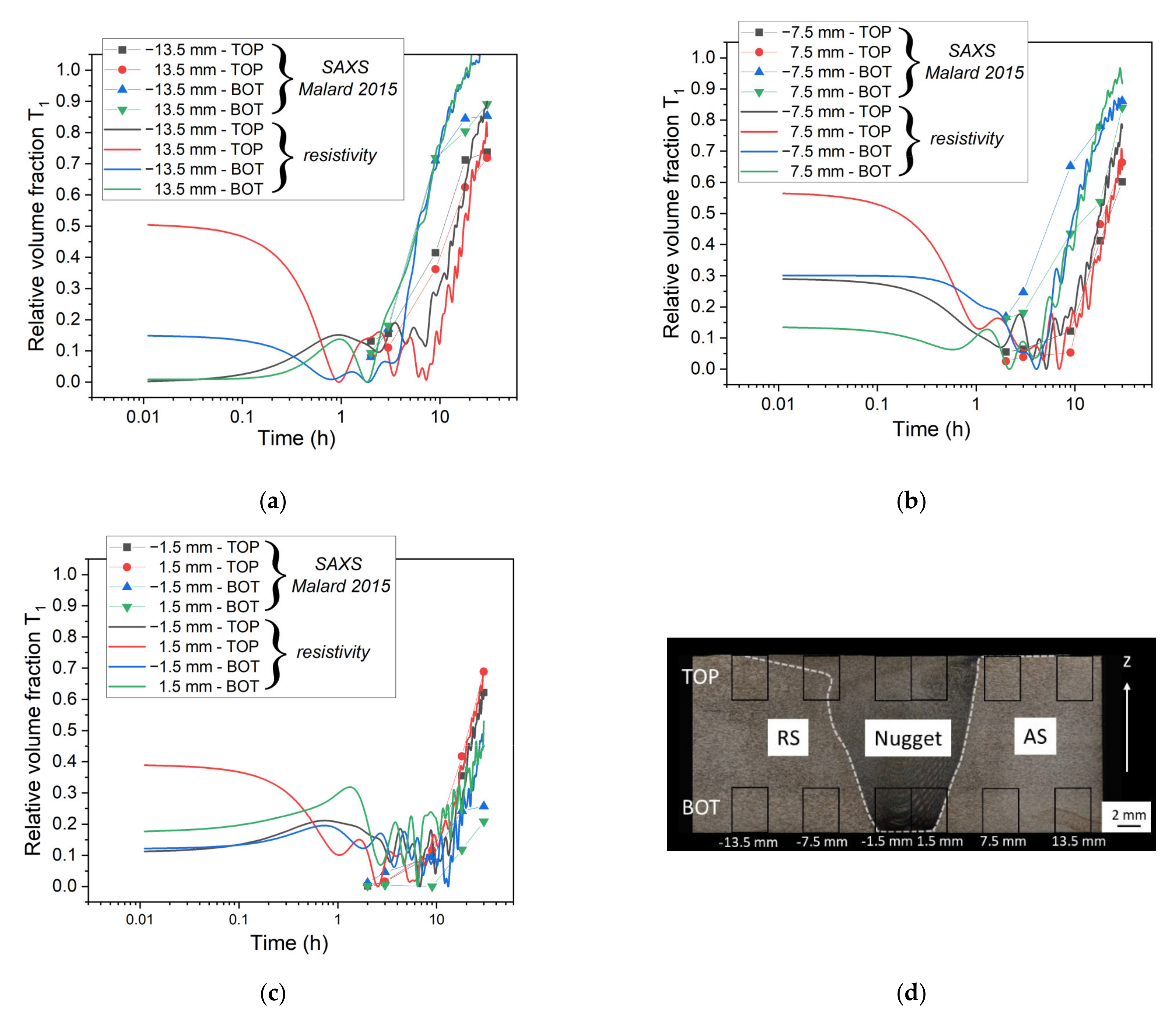
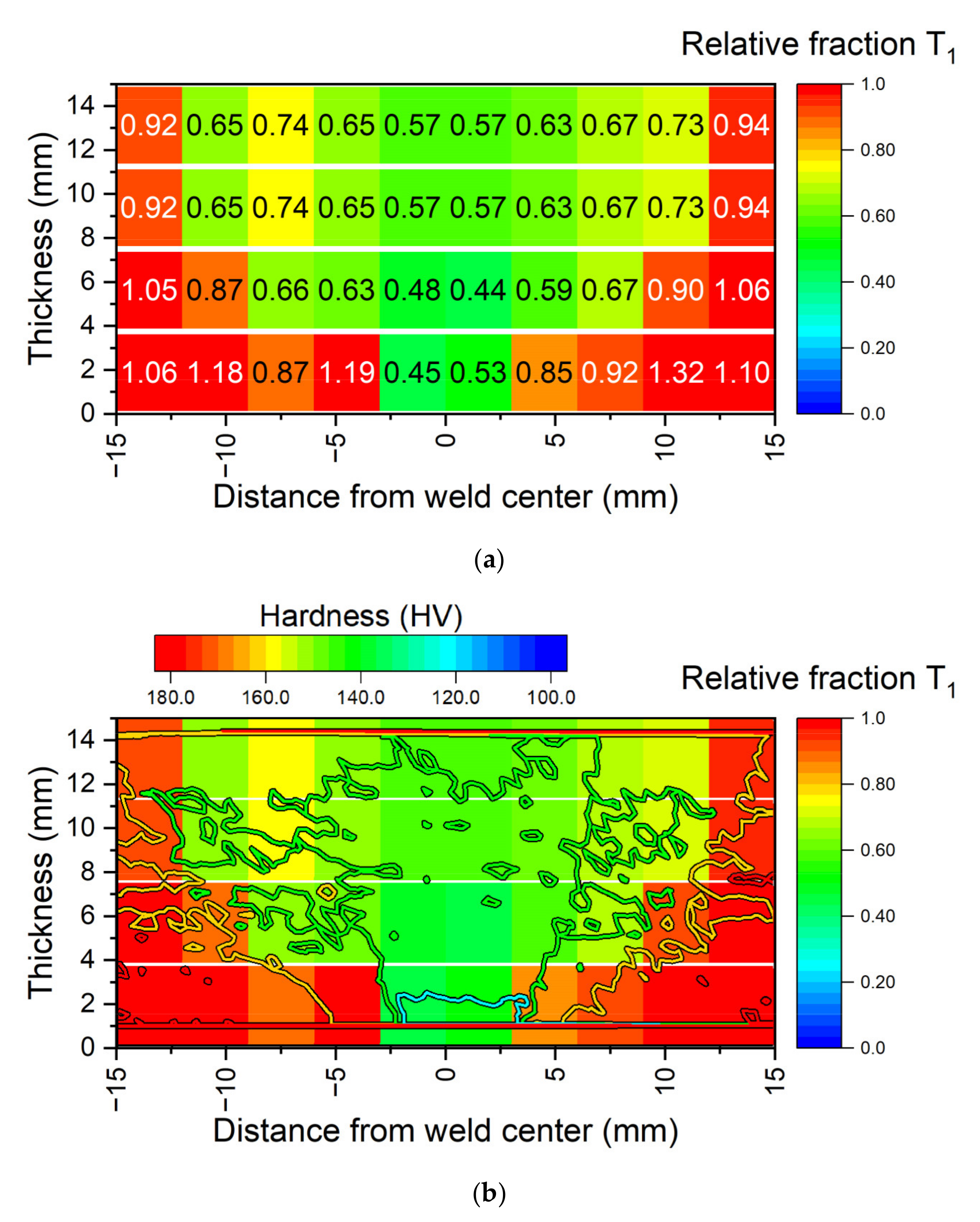
• Characterization by electrical resistivity has been performed on the unwelded material and on FSW samples to follow the precipitation kinetics of the T₁ phase during heat treatment at 155 °C. Results on FSW samples are consistent with data from the literature obtained by other techniques such as SAXS or DSC. Moreover, the softened zone in the nugget corresponds to the lower fraction of the T₁ phase obtained in electrical resistivity. This technique was thus found adequate for mapping T₁ precipitation.
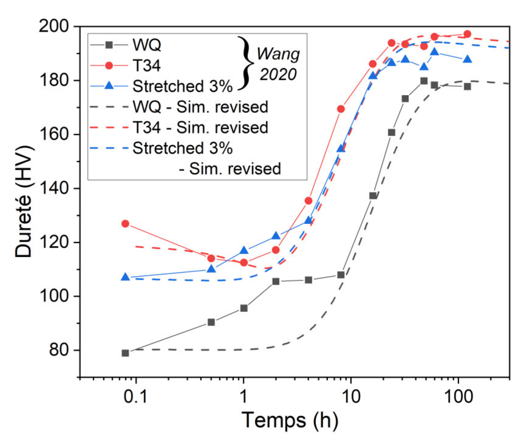
• The original constitutive model has been revised to predict the yield strength evolution during the aging of AA2050 with different initial tempers. With several modifications, the model provides proper simulations of the evolution of normalized volume fraction, normalized precipitate radius, and hardness for the different initial states.
• To simulate the evolution of the relative volume fraction of the T₁ phase and hardness in the different zones of FSW samples during post-welding heat treatment, it was chosen to impose the initial state of the material across the weld joint.
• By using experimental data from the literature to impose the initial state, a good agreement concerning the evolution of relative volume fraction until 30 h at 155 °C was found. The simulated hardness was also found to be close to experimental data but was underestimated before and after this 30 h of heat treatment.
• Finally, the resistivity measurements were used to impose the initial state of the material on the different zones of FSW samples. Despite some observed discrepancies on the top and bottom of the weld joint, the revised numerical model captures the overall hardness profile after the post-weld heat treatment.

References

1. Mishra, R.S.; Sidhar, H. Friction Stir Welding of 2xxx Aluminum Alloys Including Al-Li Alloys; Elsevier Science, Butterworth-Heinemann: Oxford, UK, 2017. [Google Scholar] [CrossRef]
2. Ahmed, M.M.Z.; Wynne, B.P.; Rainforth, W.M.; Addison, A.; Martin, J.P.; Therasgill, P.L. Effect of tool geometry and heat input on the hardness, grain structure, and crystallographic texture of thick-section friction stir-welded aluminium. Metall. Mat. Trans. A 2019, 50, 271–284. [Google Scholar] [CrossRef]
3. Hou, W.; Ding, Y.; Huang, G.; Huda, N.; Shah, L.H.; Piao, Z.; Shen, Y.; Shen, Z.; Gerlich, A. The role of pin eccentricity in friction stir welding of Al-Mg-Si alloy sheets: Microstructural evolution and mechanical properties. Int. J. Adv. Manuf. Technol. 2022, 121, 7661–7675. [Google Scholar] [CrossRef]
4. Proton, V.; Alexis, J.; Andrieu, E.; Delfosse, J.; Deschamps, A.; De Geuser, F.; Lafont, M.C.; Blanc, C. The influence of artificial ageing on the corrosion behaviour of a 2050 aluminium–copper–lithium alloy. Corros. Sci. 2014, 80, 494–502. [Google Scholar] [CrossRef] [Green Version]
5. Sidhar, H.; Mishra, R.S.; Reynolds, A.P.; Baumman, J.A. Impact of thermal management on post weld heat treatment efficacy in friction stir welded 2050-T3 alloy. J. Alloys Compd. 2017, 722, 330–338. [Google Scholar] [CrossRef]
6. Malard, B.; De Geuser, F.; Deschamps, A. Microstructure distribution in an AA2050 T34 friction stir weld and its evolution during post-welding heat treatment. Acta Mater. 2015, 101, 90–100. [Google Scholar] [CrossRef] [Green Version]
7. De Geuser, F.; Malard, B.; Deschamps, A. Microstructure mapping of a friction stir welded AA2050 Al–Li–Cu in the T8 state. Phil. Mag. 2014, 94, 1451–1462. [Google Scholar] [CrossRef]
8. Yan, Y.; Peguet, L.; Gharbi, O.; Deschamps, A.; Hutchinson, C.R.; Kairy, S.K.; Birbilis, N. On the corrosion, electrochemistry and microstructure of Al-Cu-Li alloy AA2050 as a function of ageing. Materialia 2018, 1, 25–36. [Google Scholar] [CrossRef]
9. Li, Y.; Shi, Z.; Lin, J. Experimental investigation and modelling of yield strength and work hardening behaviour of artificially aged Al-Cu-Li alloy. Mater. Des. 2019, 183, 108121. [Google Scholar] [CrossRef]
10. Avettand-Fenoel, M.-N.; Taillard, R. Heterogeneity of the Nugget Microstructure in a Thick 2050 Al Friction-Stirred Weld. Metall. Mat. Trans. A 2015, 46, 300–314. [Google Scholar] [CrossRef]
11. Wang, X.; Shao, W.; Jiang, J.; Li, G.; Wang, X.; Zhen, L. Quantitative analysis of the influences of pre-treatments on the microstructure evolution and mechanical properties during artificial ageing of an Al–Cu–Li–Mg–Ag alloy. Mater. Sci. Eng. A 2020, 782, 139253. [Google Scholar] [CrossRef]
12. Milkereit, B.; Kessler, O.; Schick, C. Recording of continuous cooling precipitation diagrams of aluminium alloys. Thermochim. Acta 2009, 492, 73–78. [Google Scholar] [CrossRef]
13. Entringer, J.; Reimann, M.; Norman, A.; dos Santos, J.F. Influence of Cu/Li ratio on the microstructure evolution of bobbin-tool friction stir welded Al–Cu–Li alloys. J. Mater. Res. Technol. 2019, 8, 2031–2040. [Google Scholar] [CrossRef]
14. Milagre, M.X.; Mogili, N.V.; Donatus, U.; Giorjao, R.A.R.; Terada, M.; Araujo, J.V.S.; Machado, C.S.C.; Costa, I. On the microstructure characterization of the AA2098-T351 alloy welded by FSW. Mater. Char. 2018, 140, 233–246. [Google Scholar] [CrossRef]
15. Thompson, G.E.; Noble, B. Resistivity of Al-Cu-Li alloys during T1 (Al2CuLi) Precipitation. Metal Sci. J. 1973, 7, 32–35. [Google Scholar] [CrossRef]
16. Yamamoto, A. Resistivity study of aging in Al-Li-Cu alloys. Mat. Trans. JIM 1995, 36, 1447. [Google Scholar] [CrossRef] [Green Version]
17. Khan, A.K.; Robinson, J.S. Effect of silver on precipitation response of Al–Li–Cu–Mg alloys. Mater. Sci. Technol. 2008, 24, 1369–1377. [Google Scholar] [CrossRef]
18. Khan, A.K.; Robinson, J.S. Effect of cold compression on precipitation and conductivity of an Al–Li–Cu alloy. J. Microsc. 2008, 232, 534–538. [Google Scholar] [CrossRef]
19. Buck, O.; Brasche, L.J.H.; Shield, J.E.; Bracci, D.J.; Jiles, D.C.; Chumbley, L.S. Nondestructive detection of the T1 phase in Al–Li alloy. Scripta Met. 1989, 23, 183–187. [Google Scholar] [CrossRef]
20. Jiang, F.; Zhang, H. Non-isothermal precipitation kinetics and its effect on hot working behaviors of an Al–Zn–Mg–Cu alloy. J. Mater. Sci. 2018, 53, 2830–2843. [Google Scholar] [CrossRef]
21. Ceresara, S.; Giarda, A.; Sanchéz, A. Annealing of vacancies and ageing in Al-Li alloys. Philo. Mag. 1977, 35, 97–110. [Google Scholar] [CrossRef]
22. Noble, B.; Thompson, G.E. Precipitation Characteristics of Aluminium-Lithium Alloys. Metal Sci. J. 1971, 5, 114–120. [Google Scholar] [CrossRef]
23. Kocks, U.F. Laws for Work-Hardening and Low-Temperature Creep. J. Eng. Mater. Technol. 1976, 98, 76–85. [Google Scholar] [CrossRef]
24. Cassada, W.A.; Shiflet, G.J.; Starke, E.A. Mechanism of AI2CuLi (T1) Nucleation and Growth. Met. Trans. A 1991, 22, 287–297. [Google Scholar] [CrossRef]
25. Shercliff, H.R.; Ashby, M.F. A process model for age hardening of aluminium alloys—I. The model. Acta Metal. Mater. 1990, 38, 1789–1802. [Google Scholar] [CrossRef]
26. Proton, V. Caractérisation et Compréhension du Comportement en Corrosion de Structures en Alliage D’aluminium-cuivre-lithium 2050 Assemblées par Friction Stir Welding (FSW). Ph.D. Thesis, Institut National Polytechnique de Toulouse, Université de Toulouse, Toulouse, France, 2012. [Google Scholar]
27. Chung, T.-F.; Yang, Y.-L.; Hsiao, C.-N.; Li, W.-C.; Huang, B.-M.; Tsao, C.-S.; Shi, Z.; Lin, J.; Fischione, P.E.; Ohmura, T.; et al. Morphological evolution of GP zones and nanometer-sized precipitates in the AA2050 aluminium alloy. Int. J. Lightweight Mater. Manuf. 2018, 1, 142–156. [Google Scholar] [CrossRef]
28. Xu, X.; WU, G.; Zhang, L.; Tong, X.; Zhang, X.; Sun, J.; Li, L.; Xiong, X. Effects of heat treatment and pre-stretching on the mechanical properties and microstructure evolution of extruded 2050 Al–Cu–Li alloy. Mater. Sci. Eng. A 2022, 845, 143236. [Google Scholar] [CrossRef]
29. Li, Y.; Shi, Z.; Lin, J.; Yang, Y.L.; Rong, Q.; Huang, B.M.; Chung, T.F.; Tsao, C.S.; Yang, J.R.; Balint, D.S. A unified constitutive model for asymmetric tension and compression creep-ageing behaviour of naturally aged Al-Cu-Li alloy. Int. J. Plast. 2017, 89, 130–149. [Google Scholar] [CrossRef]
Figure 1. Electrical resistivity measurement specimen instrumentation: (a) classical four-point method and (b) multi-point method.
Crystals 12 01543 g001
Figure 2. DSC and electrical resistivity curves for AA2050-T34 alloy with a heating rate of 20 K/min.
Crystals 12 01543 g002
Figure 3. The evolution of simulated and experimental normalized electrical resistivity vs. the relative volume fraction of the T1 phase measured by DSC.
Crystals 12 01543 g003
Figure 4. The evolution of the relative volume fraction of the T1 phase measured by SAXS by Malard et al. [6] and by electrical resistivity (this study) at the top (TOP) and the bottom (BOT) of the weld joint during the post-welding heat treatment at 155 °C and at (a) 13.5 mm; (b) 7.5 mm; and (c) 1.5 mm of the weld center. The measurement locations are shown in (d).
Crystals 12 01543 g004
Figure 5. The map of the relative volume fraction of the T1 phase in FSW weld cross-sections after the post-welding heat treatment of 30 h at 155 °C: (a) T1 phase map with figures representing the relative volume fraction originate from the multi-point resistivity measurements. (b) T1 phase and hardness map. The hardness is marked with an isoline map.
Crystals 12 01543 g005
Figure 6. A comparison between the simulation with the original model of Li et al. [9] and measurements of Malard et al. [6], Li et al. [9] and Proton et al. [26] for the heat treatment at 155 °C of AA2050-T34.
Crystals 12 01543 g006
Figure 7. The hardness evolution in WQ, T34, and Stretched 3% samples during heat treatment at 155 °C as measured by Wang et al. [11].
Crystals 12 01543 g007
Figure 8. The evolution of simulated and experimental (a) normalized radius and (b) volume fraction of the T1 precipitates in WQ, T34, and Stretched 3% samples during heat treatment at 155 °C. The original model of Li et al. [9] is used for the simulations. Experimental data comes from Wang et al. [11].
Crystals 12 01543 g008
Figure 9. The evolution of the simulated and experimental normalized volume fraction of the T1 phase during artificial aging at 155 °C with different pre-treatments. The revised model is used for the simulations. Experimental data comes from Wang et al. [11].
Crystals 12 01543 g009
Figure 10. (a) The evolution of the simulated and experimental (Malard et al. [6] and Wang et al. [11]) normalized radius vs. volume fraction of the T1 precipitates after 30 h of heat treatment at 155 °C; (b) the evolution of the simulated and experimental [11] normalized radius of the T1 precipitates during artificial aging at 155 °C with different pre-treatments. The revised model is used for the simulations.
Crystals 12 01543 g010
Figure 11. The evolution of the simulated strength contribution of the T1 precipitates during artificial aging at 155 °C. Comparison between the original [9] and revised model for the T34 state and an arbitrary slower kinetics of precipitation.
Crystals 12 01543 g011
Figure 12. The experimental and simulated hardness evolution in WQ, T34, and Stretched 3% samples during artificial aging at 155 °C. The revised model is used for the simulations. Experimental data comes from Wang et al. [11].
Crystals 12 01543 g012
Figure 13. Initial states imposed according to SAXS measurements [6] at different locations in the weld for the (a) normalized radius of clusters; (b) normalized dislocation density; and (c) maximum normalized volume fraction of non-hardening phases.
Crystals 12 01543 g013
Figure 14. The experimental and simulated evolutions of the normalized volume fraction of the T1 precipitates in the nugget at the weld center during post-weld heat treatment at 155 °C. The revised model is used for the simulations. Experimental data comes from Malard et al. [6].
Crystals 12 01543 g014
Figure 15. The experimental and simulated normalized hardness evolutions in the nugget at the weld center during post-weld heat treatment at 155 °C. The revised model is used for the simulations. Experimental data comes from Malard et al. [6].
Crystals 12 01543 g015
Figure 16. The initial states imposed according to electrical resistivity measurements at different locations in the weld for the (a) normalized radius of clusters (curves at z = 5.5 and 9 mm are superimposed); (b) normalized dislocation density (curves at z = 5.5 and 9 mm are superimposed); and (c) maximum normalized volume fraction of non-hardening phases.
Crystals 12 01543 g016
Figure 17. The experimental (electrical resistivity measurements) and simulated evolutions of relative volume fraction of the T1 phase during post-weld heat treatment at 155 °C at (a) 7.5 mm; and (b) 1.5 mm from the weld center. The revised model is used for the simulations.
Crystals 12 01543 g017
Figure 18. The experimental and simulated hardness profiles (a) at the top and bottom and (b) at the middle of the weld joint after 30 h of post-weld heat treatment at 155 °C. The revised model is used for the simulations.
Crystals 12 01543 g018