Abstract
The paper considers an algorithm for the direct search for a nonparametric smooth histogram of the particle size distribution from small-angle X-ray and neutron scattering data. The features and details of the implementation of the method, which consists in the sequential search for several solutions with different degrees of smoothness of the distribution contour, are considered. Methods for evaluating the stability of both the whole distribution contour and its individual parts are discussed. The work of the program is illustrated by examples of the analysis of polydisperse spherical particles in silicasol solutions.
1. Introduction
The properties of many modern materials are determined by structural features in the nanoscale range, so they are often investigated using small-angle scattering (SAS), X-ray scattering (SAXS), and neutron (SANS) scattering, respectively. These methods allow qualitative and quantitative investigation of the structure of matter without special sample preparation, with a resolution from angstroems to several microns. Many materials are polydisperse systems with density fluctuations lying in this range. Without loss of generality, we will hereinafter refer to the scattering fluctuations as “particles”. The analysis of such multicomponent systems is a non-trivial ill-conditioned problem, which may lead to large deviation in solutions. Thus, the condition number of the matrix of second derivatives of a minimizing target function (usually a weighted sum of squared residuals) can reach tens or hundreds of millions, which makes the solution highly dependent, not only on the errors in the input data, but also on the parameters of the search algorithm and on the initial values of the model parameters.
A number of algorithms are available for the analysis of polydisperse objects in solution from small-angle data, among which one can mention several main algorithms based on the minimization of the total quadratic discrepancy between the experimental and model scattering intensities:
- (i)
- direct search for the particle size distribution using the linear least squares method with a Tikhonov regularization of the solution (e.g., GNOM [1]—the program from the ATSAS package [2]; GIFT [3]);
- (ii)
- direct search for the particle size distribution as a histogram (McSAS random search method [4]);
- (iii)
- postulating the distribution in analytical form (e.g., normal distribution, Flory-Schulz distribution [5], etc.) and making multiparametric approximation of the data. This is implemented, e.g., in MIXTURE (and its modified version POLYMIX) [6] of the ATSAS package [2]; in SASFIT [7]); and some others.
Each of these algorithms has some advantages and disadvantages, and using only one of them does not always produce artifact-free solutions. In [8], a scheme for joint use of the algorithms was proposed to improve the reliability of reconstruction of the particle size distribution function. One of the key problems in using methods from (iii), which are most free from artifacts, is to determine the starting values of the parameters of distributions that are sufficiently close to the “correct” ones. By “correct”, we consider the mean value of a distribution parameter averaged over a large number of solutions obtained by the multistart method when varying the starting values and/or parameters of the search method. When averaging, it is recommended to discard 10–20% of the solutions that are farthest from the resulting average. The Euclidean distance between model parameter vectors or some other metric can be used as a comparison criterion.
This paper considers a nonparametric method for calculating the size distribution from small angle scattering data, which does not require a priori assumptions. The resulting solution can be definitive, or it can be used as starting values for methods of the group (iii).
2. Materials and Methods
2.1. Theory and Algorithms
2.1.1. General Principles
As a polydisperse model, the program uses a system of non-interacting particles of unit density (or the difference between the electron densities of the particle and the environment) whose dimensions are given on some grid of N radii rj from Rmin to Rmax = Dmax/2. The way of estimation of Dmax is considered below. In discrete form, the theoretical scattering intensity from such a model can be written as:
where DV(rj) is the desired (volume) distribution function; i0(s,rj) is the square of the form factor, or the scattering intensity from a particle of the given shape with radius rj, unit volume, and density contrast (we will call them partial intensities); s = [4π⋅sin(θ)]/λ—scattering vector module (2θ—scattering angle in radians, λ—radiation wavelength); v(rj)—the body volume with effective radius rj; drj—step on the radius grid. If in Formula (1), the square of the volume is used, then the distribution would be by the number of particles, DN(rj) = DV(rj)/v(rj). However, the shape of the DN(rj) graph is uninformative due to the rapid decay of the curve with increasing radius and, therefore, it is not used.
The type of particle shape can be chosen: spheres, ellipsoids, cylinders, disks, multi-layer and hollow bodies, as well as a user-defined formfactor stored in an external file. Formulas for calculating scattering intensities from different geometric bodies and other models of particle structures can be found in [9,10]. In this paper, we will limit ourselves to the form factor of a homogeneous sphere (most commonly used in practice) with unit contrast and volume:
The minimized target function corresponds to a least squares problem
where
i = 1, …, M being the index of the angular point in the data. x is the vector of length N (vector of parameters) of the current DV(r) distribution values; I(s) is the theoretical intensity according to formula (1); w(s) is the weight function compressing the intensity range (see below); ξ is an auxiliary least-squares multiplier matching the scattering curves before calculating the difference
where is the scalar product of vectors of weighted experimental and theoretical intensities. This multiplier allows the program to deal only with fitting the shape of the intensity curve, not its absolute values. This improves the conditionality of the problem.
The arguments x of the target function (Equation (3)) are the values of the centers of the boxes on the histogram of the distribution represented on the grid of N particle radii from 0.1 nm to Dmax. The grid spacing in the program is equidistant. Smaller size step in the region of small sizes (for example, for the grid with the increasing relative step) is ineffective because scattering from small particles in the experimental region of angles is represented by almost similar weakly decreasing monotonous curves. The corresponding matrix of intensities in this case is close in character to the Hilbert matrix, which is characterized as a very ill-conditioned one. Consequently, the set of form factors of small particles can be degenerate within the accuracy of the machine arithmetic, and the relative small size step is unreasonable.
In the case of scattering from polydisperse systems, Dmax can be obtained with an acceptable accuracy from the estimate of the maximum radius of inertia of particles Rg from the Guinier plot in the low angle region in the spherical approximation of the shape of scattering particles [9]:
Here, n = 3 for spherical formations, 2 for radius of inertia of cross-section of an elongated particle, and 1 for radius of inertia of cross-section of disk-shaped particles. Estimation of maximum size for spherical particles can be put equal to
It might seem that in the case of spherical particles, Dmax should be assigned equal to . However, the approximation (5) is only accurate for . Since it is calculated from scattering data starting from smin > 0, it could be an underestimate, especially if the system contains a small fraction of large particles. Therefore, the estimate (6) is set as the minimum large value not yet leading to unreasonable overestimation of the model intensity in the region of extrapolation [0: smin]. In practice, (6) is a good choice for nonspherical particles as well.
The basic ideas of the solution search algorithm in the VOLDIS program are as follows.
- (1)
- The search for the minimum discrepancy between the experiment and the model (Equation (3)) is performed by the fast Levenberg-Marquardt method (a modified DN2FB procedure [11]), which is a variant of the NL2SNO algorithm [12], with constraints on the variables.
- (2)
- The program directly changes the distribution values at each node of the histogram. However, this distribution will consist of a large number of narrow peaks due to the strong correlation of the scattering intensity curves of neighboring (i.e., close in size) particles.
- (3)
- To suppress the splitting of broad distribution peaks into a large number of closely spaced narrow bands, the model scattering intensity in (3) is calculated from a smoothed distribution contour. This method additionally improves the conditionality of the problem.
- (4)
- The program finds a series of five to ten solutions with different (increasing from solution to solution) degrees of smoothing of the distribution contour. The search iteration for each subsequent solution starts with the smooth contour obtained at the previous iteration.
- (5)
- From the obtained set of solutions, the user chooses the smoothest distribution using an acceptable quality criterion of fitting (χ2, residual autocorrelations criterion, etc.).
- (6)
- The obtained distributions are averaged, discarding the solutions for which the quality criterion does not exceed twice the value of the best one. In the process of averaging, absolute values of deviations between successive distributions are accumulated. These values are assumed to be the error bars in the DV plot. When averaging, strongly oscillating distributions can be discarded by specifying the interval of solution indices.
- (7)
- In order to avoid artifacts in the area of large sizes, the model intensity in the extrapolation region to the zero scattering angle is calculated and analyzed. If this region of Dv decreases non-monotonically by the 2nd derivative criterion, the program gives a message about the necessity to decrease Dmax (by default—by a factor of 1.5).
- (8)
- The uniform particle number distribution is used as the starting approximation. From the 2nd iteration, distribution starts from the smoothed contour obtained at the previous step. It is possible to start a new iteration from the initial approximation.
- (9)
- Distributions are searched for in the range [DVmin: 104], where DVmin is set to zero or a small number. The upper limit protects against numerical overflow. Dynamic normalization of distributions in the search process proved to be unacceptable due to a deterioration in the conditionality of the problem. In addition, this sometimes leads to its multimodality. Restrictions on the non-zero minimum values DVmin in the histogram may be set using information about the nature of the sample under study: sometimes it is necessary to consider the impossibility of a strict absence of particles of any size, then the presence of a non-zero background in the distribution can be introduced. Of course, the shape of such a background curve must depend on the type of the particular object and is not considered in this manuscript.
2.1.2. Minimization Method
In contrast to the well-known McSAS direct search method [4], a modified version of the Levenberg-Marquardt algorithm [[12,13] (Chapt. 4.7.3)] is implemented in the program VOLDIS to find the minimum of the target function. The Monte Carlo method is used in the McSAS program, the convergence speed of which depends on the average step of variation of the model parameters values and can be many times worse than the first-order methods based on the use of local gradient estimates of the target function. The globality property of the Monte Carlo method does not play a role in our case, since even if the minimized function is multimodal, the distance between local minima exceeds by orders of magnitude the optimal value of parameter variation in random search methods. There is a simulated annealing method for such cases, but our practice has also shown its inefficiency as the only search procedure. On the other hand, the program with the quasi-Newton search algorithm works with the same, or even smaller, time costs and higher probability of finding the global extremum when a multistart strategy is used.
Briefly, the Levenberg-Marquardt algorithm (see [13], Chapt. 4.7.3) uses the matrix of first derivatives J of the vector target function (Equation (3)) to estimate the approximation to the matrix of second derivatives H. If xk is the current point at the k-th iteration (the vector of distribution in our case), then, in the linear least-squares case, the point of minimum function is reached if the step pk is taken from the equation (Newton’s method) as
If the norm of residuals is less than the maximum eigenvalue of the matrix T (see [13], Chapt. 4.7.1), using T instead of H in the expression for Q(x) (Equation (7)) can provide a convergence speed close to the quadratic one for nonlinear problems, even if one neglects the second order term Q(x). This leads to the Levenberg-Marquardt method: pk is taken according to equation
where E is unit matrix, α is a positive number which provides some improvement in the conditionality of matrix T, and increases the stability of the search in the case of nonlinear least squares problems. The parameter α is chosen in the program automatically from the descent requirement ([13], Chapt. 4.7.3).
2.1.3. Modification of the Minimization Procedure
The original code of the minimization program DN2FB [11] has been modified. Since this modification is important to ensure the performance of the method, consider it in a bit more detail.
An automatic evaluation of optimal values of finite-difference parameter increments was added to estimate the first derivatives. If there are significant (in comparison with the machine accuracy) errors in calculating the values of the target function, the parameter increments should be increased. By default, they are usually set equal to , where EPS ≈ 2.22 × 10⁻¹⁶ is the relative accuracy of double precision machine arithmetic, xi–current value of the i-th parameter of the model. In practice, instead of EPS, it is necessary to use accuracy of calculation of values of the target function. Accuracy here refers to the magnitude of fluctuations in the function value obtained with small argument increments. The errors are due to the total of rounding errors accumulated in the course of all calculations. Let’s call this error “calculation noise”, εF. Unfortunately, the necessity of estimating εF is not emphasized in known software packages. Calculation noise influences the efficiency of minimization programs, since at too small (or too large) parameter variations the calculation of gradients becomes meaningless, and the search stops farther from the minimum the greater the noise. It is impossible to predict εF analytically, because even if such estimates exist, they are usually upper-bound values and have no practical sense. But it is possible to make an estimate “on the fact” by making M small variations of model parameters and analyzing the set of values of the target function, writing them in the vector f0. In practice, the number of variations M = 15–20 for each parameter is sufficient. The values of variations for the variables x are chosen from the approximate condition of optimal increment for the third derivative of the target function in the absence of additional information as [13]. It should be noted that the algorithm for calculating computational noise is a little sensitive to the choice of the magnitude of the increment. It can be varied within two to three orders of magnitude or even more.
The obtained values of f0 are entered in the first column of the finite difference table. The next columns contain the values of differences of two consecutive elements of the previous column, obtaining first, second, third, etc., difference columns. In [14] (Chapt. 1.4 and 2.8), it is shown that, if in the column of n-th differences the signs of consecutive elements alternate (i.e., the correlation coefficient of consecutive elements tends to −1), then their values are due to the random variations in the first column. Knowing the order of differences n, from the value of the standard deviation σn of elements in this column, we can reverse the calculation of the relative random deviation in the target function (first column) as:
Here is the mean function value for which the estimate is made.
Now, we can compute the optimal increment of the i-th argument for the one-sided finite-difference first derivatives scheme which is used in the DN2FB algorithm as
As shown in [13], such an estimate approximately minimizes the sum of the errors in , the first of which is due to computational noise and the second to the error of the finite difference scheme itself. Optimal relative increments of arguments of the target function considered in this paper in practice lie in the range 10−6–10−3, depending on the type of the form factor, whereas, in the standard way, the assigned increments would be 10−7–10−8 in double precision calculations, which would lead to inoperability in the search procedure.
2.1.4. Details of the VOLDIS Algorithm Implementation
Maximum Diameter and Scattering Extrapolation to Zero Angle
The essential difference of the VOLDIS algorithm is that the program analyzes the curvature of the graph of the theoretical scattering intensity in the range of extrapolation to zero scattering angle after the preliminary solution search. The point is that the overestimation of the maximum particle diameter often results in the interpretation of the initial experimental section of the scattering curve as a right slope of the first scattering maximum from the narrowly dispersed fraction of very large particles which are actually absent. In this case, artifacts appear in the distribution in the form of a narrow fraction of large particles, with a mean radius of inertia much higher than the estimate (5). The extrapolated region of the model scattering curve decreases nonmonotonically (i.e., the second derivative changes its sign, whereas this region should be convex upwards). The VOLDIS program provides analysis of the extrapolation area shape in order to give a warning that, in case of its non-monotonicity, the maximum size in the histogram should be reduced by 1.5–2 times. The described analysis is important if an external formfactor is used for which it is difficult to a priori establish effective maximum expected size. Unfortunately, machine learning algorithms are unsuitable for such analysis because of the highly variable nature of the reference examples.
As noted at the end of Section 2.1.1, rule (6) for selecting the upper bound of the distribution works satisfactorily in practice in most cases.
Smoothing of the Distribution Contour and the Number of Histogram Nodes
The number of points on the distribution curve can reach values as high as 300. Its reduction to 50 or less leads to the fact that the superposition of form factors (1) is no longer monotonous enough to adequately represent the scattering curve shape. The default value chosen in the program is 200. The computation time is directly proportional to the number of points in DV.
However, at small radius steps, the shapes of the scattering intensity curves for close-sized particles are so similar that, during the search, the increased contributions from particles of the same radius are compensated by decreased contributions from particles of nearby radii without significant changes in the theoretical scattering curve. This leads to a distribution comprising several dozen narrow maxima, which does not have any physical sense. For that reason, VOLDIS computes the theoretical scattering curve from a smoothed distribution contour and searches for a set of solutions with varying degrees of smoothing. The simplest nonparametric moving average algorithm with a Hamming kernel is used as a smoothing method [14,15]. The kernel is understood as a bell-shaped weight function, ui, applied inside a window of width K = 2k + 1 points with indexes i − k, …, i + k, in which a weighted average is calculated subject to , with . The shape of the Hamming window u is one period of cosine from –π to π, shifted along the ordinate to the positive region. The width of the window K (degree of smoothing) varies between 1 and 10% of the full distribution range, but not less than 3 points. The program uses an original approach consisting of smoothing that is carried out five to ten times sequentially, which excludes the bumps on the smoothed profile that can occur during one-pass smoothing. During program development, spline-smoothing algorithms and the best piecewise polynomial schemes were tested, with different types of weighting and regularization. These approaches did not reveal any advantages.
Solution Quality Criteria
From the obtained solutions, we select the smoothest distribution corresponding to the magnitude of χ2, which does not exceed the value obtained with the minimum degree of smoothing by more than 1.5 times. Further, the corresponding model intensity should describe the experimental data without systematic deviations exceeding the standard deviation of noise in the data by more than 1.5 times.
Pay attention that the χ2 criterion makes statistical sense only in the case of adequate evaluation of standard deviations in experimental data. Sometimes these estimates are absent or equal to zero in the case of model problems. But, even in the latter case, model intensities are calculated with finite accuracy, i.e., they contain some “calculation noise”. In such cases, a criterion of “residuals randomness” may be used. The program employs the Durbin-Watson test [16] to check the residuals for autocorrelations between consecutive elements, which are calculated using the formula:
where Fi is the tested sequence Iexp – Imod. The value of the criterion lies in the region of {0–4}, taking values of about 2.0 in the case of no correlation. Thus, if the hypothesis of the presence of correlation between successive elements of the array has a significance level of 0.05, it is rejected if the criterion value lies in the range {1.8–2.2}. Of course, the statistically valid value depends on the number of elements in the sequence but, for our purposes, we can neglect the statistical rigor of the estimates. In practice, it is necessary to admit the presence of weak residual correlation due to instrumental distortions and other systematic measurement errors and, in most cases, the boundary should be slightly extended (for example, to {1.6–2.2}), justifying this extension empirically on the basis of experience of solving similar problems. Such an extension is not strict but refers to expert estimates. So, DW < 1.6 correspond to systematic deviations of the residuals. This usually corresponds to too high a degree of smoothing of the distribution. If DW > 2.2, then the solution is most likely adequate. Due to the high monotonicity of the small-angle scattering curves, no model will be able to describe the frequent systematic intensity fluctuations, which represent the high-frequency spectral component of the noise. In this case, the nature of the experimental noise is not accidental—the noise fluctuations change sign too often, which leads to negative autocorrelations in them. Estimate (11) can be used as an integral criterion, calculating it for the whole angular range of data, or we can apply a window criterion, calculating (11) inside a scanning window 10–20% of the whole range. In the latter case, we will obtain a curve of DW estimates in which areas with DW < 1.6 correspond to systematic deviations. This is extremely useful information, since on the basis of the obtained statistics, one can construct an additional weight function for Iexp, increasing the contribution of the corresponding scattering regions to (3) and repeating the search from scratch.
Intensity Weighting
Finding a model by minimizing the quadratic deviation usually implies weighting the data by multiplying the intensity by the value inverse of the standard deviation estimate. Then, the solution quality criterion is the minimal deviation of χ2 value from one. Such a solution corresponds to the maximum likelihood criterion, which seems attractive because of its name and statistical meaning. However, in the case of SAS data analysis, this correct approach often fails. The problem is that the model intensity is fitted within an aligned error corridor. In this case, the shape of the weighted scattering curve becomes dependent on the type of detector (one-dimensional, sectoral, or two-dimensional). As a rule, the experimental data are dominated by Poisson noise, in which the standard deviation equals the square root of their mathematical expectation (~mean intensity). Then, the intensity obtained by azimuthal averaging of the isotropic pattern of the two-dimensional detector will have significantly less relative noise compared to the one-dimensional detector at large angles. However, this region contains mostly atomic scattering background and non-informative tails of particle scattering. In addition, the intensity at large angles can be incorrect due to slightly incorrect subtraction of the scattering from an empty cuvette or a cuvette with solvent. Consequently, the requirement for high absolute accuracy of the fit at large angles can be made weaker. The practice of solving a large number of model and real problems has shown that the solution of the distribution search problem weakly depends on the starting approximation if the ratio of the maximum intensity (at small angles) to the minimum intensity (at large angles) is within five to ten, i.e., the curve weighting should simply reduce this ratio to the required level, regardless of the error amplitude distribution along the data curve. The influence of a significant noise component at large angles will be small if the number of angular samples is more than five to ten times the number of Shannon channels in the data, which is usually fulfilled in practice. Under the Shannon channel, we mean the maximum allowable angular step at which there is still no loss of information. It is defined by the maximum size Dmax of particles as sshann = π/Dmax [9] (Chapt. 3.2). Then, the number of Shannon channels is Nshann = (smax − smin)/sshann. In practice, the number of angular samples N > 10 Nshann is a good choice.
The range of scattering intensities can be compressed in different ways. First, it is possible to calculate the discrepancies (Equation (3)) in coordinates I(s) s2: s (so called Kratkis plot) or even I(s) sp, where p is a real exponent value. In the case of the analysis of monodisperse systems, such weighting of the data additionally attenuates the relative contribution to the non-conformity of the initial part of the scattering curve, where an undesirable contribution of scattering from particle aggregates is possible. In the case of polydisperse systems, however, the initial angular section already contains basic information about the shape of the distribution. In order not to lose the contribution of the scattering from the large particles, one can artificially increase the scattering at initial values of s by means of additional multipliers, as conducted, for example, in [17].
Second, as it is sometimes conducted, it is possible to calculate the quality criterion by calculation of residuals in the logarithmic scale of intensities. Practice has shown that the better way to weight intensities is to rise them to a real power less than unity. However, both logarithm and exponentiation are nonlinear operations, which, in case of medium and large noise in the data, significantly shift the mathematical expectation of the intensity. But these transformations can be reduced to linear operations as follows. The experimental scattering intensity curve Iexp is smoothed until there is no autocorrelation in the residuals (see above). The smoothed curve Ismo(s) is raised to the required real degree p obtaining . The ratio is calculated. After multiplying Iwork(si) = Iexp(si) u(si), the working intensity curve is close in its shape to {Iexp(si)}p, but it is obtained as a result of a linear transformation. We have called such an operation a “quasi-power” transformation. A similar approach can be applied to the “quasi-logarithmic” transformation.
“Quasi-transforms” have some disadvantage consisting in the growth of the relative amplitude of noises, but, as noted above, when the number of points on the scattering curve is large enough, such noises do not lead to a noticeable growth of the solution bias.
On the Choice of Formfactor Type
The question about the adequacy of the choice of the formfactor is discussed in many publications (for example—in [4]). Our practice of solving model problems shows that, in the case of slightly anisometric particles with a ratio of maximum and minimum radii of 2:1–3:1, the shape of distribution is close to the true one if we use the spherical approximation. As mentioned in Section 2.1.1, the user can set the particle form factor as an external file containing the scattering intensity from a particle with a given structure in case of spherically symmetric bodies–with a given radial electron density distribution function, with the size corresponding to Dmax, and with the maximum scattering angle equal to the experimental one. Scattering from the intermediate sizes will be calculated by scaling the given template intensity downward using spline interpolation. The number of points in the template formfactor data should not be less than 3000–5000 to ensure acceptable accuracy of handling sharp breaks in the curve.
Note that the simultaneous use of multiple formfactors and a representation of the scattering intensity as a superposition of independently computing histograms leads, in the case of a nonparametric approach, to such ill-conditioned problems that the solution is completely ambiguous. In order to solve a problem with several types of form factors, it is necessary to “assemble” the distributions of similar particles into maximally compact sets using analytical expressions of distributions, as implemented (for example—in the program MIXTURE [2,6]). In turn, a good starting approximation of the parameters of the distributions for this program can be obtained from the analysis of VOLDIS solutions using the simplest spherical case.
Assessment of Stability of Distribution Shapes
To assess the stability of solutions, we tested a number of criteria based on the calculation and accumulation of pairwise correlation coefficients and nonparametric criteria that test hypotheses of a consistent monotonic change in the contours of distributions. The criteria were calculated within a running window that represents 5–15% of the entire size range. Both a rectangular window and a window with a Hamming bell-shaped weight function were used. Neither approach has yielded acceptable results so far. Therefore, the simplest approach, based on averaging solutions within a given range of iterations and accumulation of pairwise differences between curves, is now implemented in the program. Only solutions whose quality criterion (χ2 or R-factor) does not exceed the minimum value obtained by a factor of 1.5–2 are involved in the averaging process. Of course, the search for effective criteria will continue.
Other Details
The program includes a mode of fitting a constant that is subtracted from the experimental intensity to compensate for the atomic scattering background. In this case, the contribution to the distribution of particles with radii less than 2–5 Å decreases by orders of magnitude, and the distribution of particles with larger radii becomes more stable.
2.2. Measurement Details
Intensity of scattering was measured on the laboratory small-angle diffractometers AMUR-K and HECUS SYSTEM-3. The diffractometers were equipped with linear position-sensitive gas detectors and fine-focus X-ray tubes with copper anodes (wavelength 0.1542 nm). The X-ray beam cross section was 0.2 × 8 mm. The sample-detector distance was 700 mm for AMUR-K and 280 mm for HECUS, covering 0.1 < s < 10.0 nm−1 and 0.1 < s < 6.5 nm−1 for each of the instruments, respectively. The samples were placed in quartz capillaries of 1 mm diameter (sample thickness). The measurement time for one sample was 10 min. The experimental data were corrected for collimation distortions, as described in [9] (Chapt. 9.4). The scattering intensity from the capillary with the solvent was subtracted from the sample scattering data.
2.3. Sample Description
0.05% aqueous solutions of Ludox TM50 silica particles (Grace Davidson) [18] were used as the study object. The weight concentration of the particles in the measured samples was chosen from a series of small angle scattering experiments as the maximum concentration at which the effect of interparticle interference distorted the initial part of the scattering curve by not more than 0.1%. The particles are stabilized at the concentration of NaOH 0.06 M. The negative charge of dissociated silanol groups SiO− on the surface of silica nanoparticles attracts Na+ cations, which form a charged layer close to the surface of the silica called the stern layer. Such charged layers lead to stable colloid suspension due to strong electrostatic repulsion between the particles [19].
2.4. Additional Software
The data were pre-processed using the ATSAS software package [2,20]. The pre-processing sequence is discussed in detail in [9] (Chapt. 9). The corresponding operations are performed in the PRIMUS package, which is described in [21], and examples are presented on the ATSAS website.
3. Results and Discussion
According to official data, the average diameter of TM50 nanoparticles is 22 nm [18], while the analysis of scattering data showed a larger mean value, 26 ± 1 nm (Figure 1, Figure 2 and Figure 3). It can be assumed that, in aqueous solution, the particles are heterogeneous and their shell, due to hydrolysis, contains polysilicic acids, which increase the diameter determined from the X-ray scattering data. In addition, Na+ ions and OH− groups form a double electric shell on the surface of the nanoparticles in solution, which prevents their aggregation and increases contrasts of their surface, thus increasing the determined diameter in solution. It can be assumed that the indicated diameter of 22 nm is obtained from electron microscopy data from dry nanoparticles. In [22], the data obtained for the TM50 solutions by acoustic spectrometer (32.1 nm), by laser diffraction (29.9 nm), and by dynamic light scattering (34.1 nm) are given. Such discrepancy of published data allows one to assert that the particle size found from data of small-angle X-ray scattering is the most adequate.
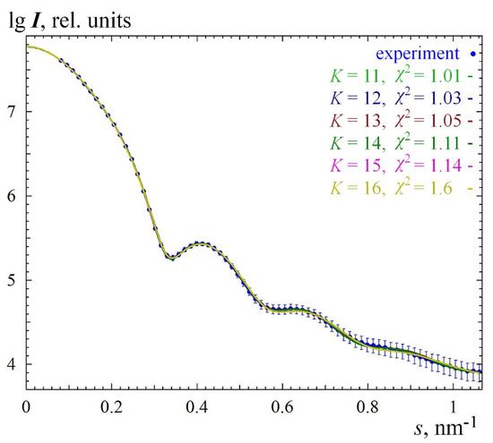
Figure 1.
Experimental (dots, smoothed by nonparametric adaptive algorithm) and model (solid lines) intensities of small angle scattering from silica sample TM50. Final solution (Figure 3) is chosen to be as smooth as possible when χ2 is still small (in this case χ2 = 1.11). K denotes the width of the smoothing window in points.
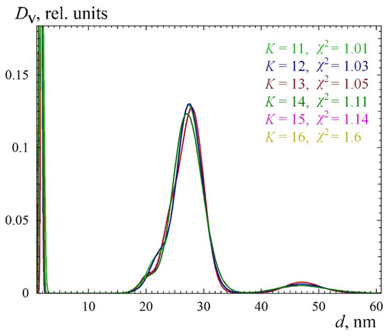
Figure 2.
The set of size distributions calculated at different degrees of smoothing. The widths of the smoothing windows are indicated in points. The average diameter of the main fraction is 26 ± 1 nm. The distribution of the main fraction is asymmetrical and is a superposition of distributions of nanoparticles with average diameters of 22 ± 0.5 and 27 ± 0.5 nm. Contributions of particles with average radii of 47 ± 2 nm and 1.5 ± 0.5 nm are also visible. The shape of the distributions for larger diameters weakly depends on the degree of smoothness of the distribution, whereas the distribution of the smallest particles at 1.5 nm is less stable.
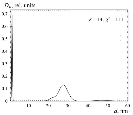
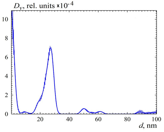
Figure 3.
Ludox TM50 silica nanoparticles size distribution proposed as the final solution.
Figure 4 and Figure 5 show a case of calculated distribution with erroneously overestimated maximum size. This was another measurement of a TM50 sample in which the particles were dissolved in distilled water without the addition of NaOH. The formation of aggregates was assumed, so the maximum diameter was increased to 100 nm, and the corresponding form factor was calculated, which the program read from an external file. This form factor was calculated from a radial distribution function, which took into account the possible presence of a polyacid shell with a thickness of 10% and an average density of 0.7 (the density of the quartz core was assumed to be 1). We will not give here all the details of the experiment and its justification. This is the subject of a separate article. What is important for us, here, is that the maximum size turned out to be really overestimated. Figure 4 shows scattering from all solutions, which show that, at a small degree of distribution smoothing, the extrapolation area (to the zero angle) is nonmonotone. As the degree of smoothing increases, this effect decreases until it disappears, but a solution that is too smooth no longer fits the experiment. Nevertheless, five solutions were selected for averaging, and the result is shown in Figure 6. You can see that the main peak of the distribution is almost similar to the one shown in Figure 3. The peak in the region of larger sizes showed a large instability between the solutions, that is, it can be considered an artifact of the overestimated maximum diameter of the particles.
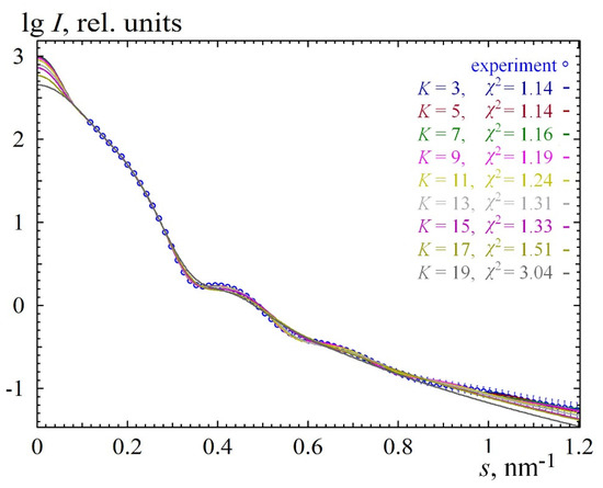
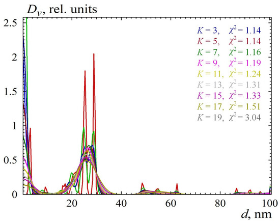
Figure 5.
The set of all solutions for the data in Figure 4.
In this manuscript, the results of working with the program are demonstrated on a relatively simple example of a narrowly dispersed particle distribution for which there is size information obtained using other methods. But the considered peculiarities of the solution search are also fully valid for considerably polydisperse systems, which have a characteristic distribution close to fractal. Some details about the search procedure can be found also in [8].
Funding
This work was funded by the BioSAXS Group with regard to software development, and it was partially supported by the Ministry of Science and Higher Education within the state assignment FSRC «Crystallography and Photonics» RAS regarding sample preparation and data treatment. The measurements were performed using the equipment of the Shared Research Center FSRC “Crystallography and Photonics” RAS, and this work was supported by the Russian Ministry of Science and Higher Education (project RFMEFI62119X0035).
Institutional Review Board Statement
Not applicable.
Informed Consent Statement
Not applicable.
Data Availability Statement
Information on the sizes of silica particles can be found in [19,22]. The original code of the DN2FB minimization program can be found in [11]. In this paper, the code was modified as described in Section 2.1.3.
Acknowledgments
The author is grateful to Petr V. Konarev and Sergey V. Amarantov for fruitful discussions on the details of the algorithm and to Viktor E. Asadchikov for recommendations on the whole work.
Conflicts of Interest
The author declares no conflict of interest. The funders had no role in the design of the study; in the collection, analyses, or interpretation of data; in the writing of the manuscript; or in the decision to publish the results.
References
- Svergun, D.I. Determination of the regularization parameter in indirect–transform methods using perceptual criteria. J. Appl. Cryst. 1992, 25, 495–503. [Google Scholar] [CrossRef]
- Manalastas-Cantos, K.; Konarev, P.V.; Hajizadeh, N.R.; Kikhney, A.G.; Petoukhov, M.V.; Molodenskiy, D.S.; Panjkovich, A.; Mertens, H.D.T.; Gruzinov, A.; Borges, C.; et al. ATSAS 3.0: Expanded functionality and new tools for small-angle scattering data analysis. J. Appl. Cryst. 2021, 54, 343–355. [Google Scholar] [CrossRef] [PubMed]
- Brunner-Popela, J.; Glatter, O. Small-Angle Scattering of Interacting Particles. I. Basic Principles of a Global Evaluation Technique. J. Appl. Cryst. 1997, 30, 431–442. [Google Scholar] [CrossRef]
- Bressler, I.; Pauw, B.R.; Thünemann, A.F. McSAS: Software for the retrieval of model parameter distributions from scattering patterns. J. Appl. Cryst. 2015, 48, 962–969. [Google Scholar] [CrossRef] [PubMed]
- Flory, P.J. Molecular Size Distribution in Linear Condensation Polymers. J. Am. Chem. Soc. 1936, 58, 1877–1885. [Google Scholar] [CrossRef]
- Svergun, D.I.; Konarev, P.V.; Volkov, V.V.; Koch, M.H.J.; Sager, W.F.C.; Smeets, J.; Blokhuis, E.M. A small angle X-ray scattering study of the droplet–cylinder transition in oil–rich sodium bis(2–ethylhexyl) sulfosuccinate microemulsions. J. Chem. Phys. 2000, 113, 1651–1665. [Google Scholar] [CrossRef]
- Bressler, I.; Kohlbrecher, J.; Thünemann, A.F. SASfit: A tool for small-angle scattering data analysis using a library of analytical expressions. J. Appl. Cryst. 2015, 48, 1587–1598. [Google Scholar] [CrossRef] [PubMed]
- Kryukova, A.E.; Konarev, P.V.; Volkov, V.V.; Asadchikov, V.E. Restoring silicasol structural parameters using gradient and simulation annealing optimization schemes from small-angle X-ray scattering data. J. Mol. Liquids 2019, 283, 221–224. [Google Scholar] [CrossRef]
- Feigin, L.A.; Svergun, D.I. Structure Analysis by Small-Angle X-ray and Neutron Scattering; Plenum Press: New York, NY, USA, 1987; p. 321. [Google Scholar]
- User Guide for the SASfit Software Package. Available online: https://raw.githubusercontent.com/SASfit/SASfit/master/doc/manual/sasfit.pdf (accessed on 5 November 2022).
- Available online: http://www.netlib.no/netlib/port/dn2fb.f (accessed on 3 January 2005).
- Dennis, J.E., Jr.; Gay, D.M.; Welsh, R.E. Algorithm 573 NL2SOL—An Adaptive Nonlinear Least–Squares Algorithm [E4]. ACM Trans. Math. Soft. 1981, 7, 369–383. [Google Scholar] [CrossRef]
- Gill, P.E.; Murray, W.; Wright, M.H. Practical Optimization; Academic Press: London, UK, 1982; p. 462. [Google Scholar]
- Hamming, R.W. Numerical Methods for Scientists and Engineers; Mc Graw-Hill Book Company, Inc.: New York, NY, USA, 1962; 411p. [Google Scholar]
- Bowman, A.W.; Azzalini, A. Applied Smoothing Techniques for Data Analysis; Claredon Press: Oxford, UK, 1997; p. 193. [Google Scholar]
- Durbin, J.; Watson, G.S. Testing for Serial Correlation in Least–Squares regression III. Biometrika 1971, 58, 1–19. [Google Scholar] [CrossRef]
- Svergun, D.I. Restoring Low Resolution Structure of Biological Macromolecules from Solution Scattering Using Simulated Annealing. Biophys. J. 1999, 76, 2879–2886. [Google Scholar] [CrossRef]
- Available online: https://www.chempoint.com/products/grace/ludox-monodispersed-colloidal-silica/ludox-colloidal-silica/ludox-tm-50 (accessed on 2 January 2002).
- Sögaard, C.; Funehag, J.; Abbas, Z. Silica sol as grouting material: A physio-chemical analysis. Nano Converg. 2018, 5, 6. [Google Scholar] [CrossRef] [PubMed]
- Data Analysis Software ATSAS 3.1.3. Available online: https://www.embl-hamburg.de/biosaxs/software.html (accessed on 9 September 2022).
- Konarev, P.V.; Volkov, V.V.; Sokolova, A.V.; Koch, M.H.J.; Svergun, D.I. PRIMUS—A Windows-PC based system for small-angle scattering data analysis. J Appl Cryst. 2003, 36, 1277–1282. [Google Scholar] [CrossRef]
- LUDOX® Colloidal Silica, Grace—ChemPoint. Colloidal Silica as a Particle Size and Charge Reference Material. Available online: https://www.horiba.com/fileadmin/uploads/Scientific/Documents/PSA/TN158.pdf (accessed on 10 November 2019).


Publisher’s Note: MDPI stays neutral with regard to jurisdictional claims in published maps and institutional affiliations. |
© 2022 by the author. Licensee MDPI, Basel, Switzerland. This article is an open access article distributed under the terms and conditions of the Creative Commons Attribution (CC BY) license (https://creativecommons.org/licenses/by/4.0/).