
The Correspondence Theory and Its Application to NiTi Shape Memory Alloys


EPFL (Ecole Polytechnique Fédérale de Lausanne), LMTM, PX Group Chair, 2000 Neuchatel, Switzerland
Crystals 2022, 12(2), 130; https://doi.org/10.3390/cryst12020130
Submission received: 23 November 2021
/
Revised: 11 January 2022
/
Accepted: 13 January 2022
/
Published: 18 January 2022
(This article belongs to the Special Issue Crystallography of Structural Phase Transformations (Volume II))
Abstract
:Martensite crystallography is usually described by the phenomenological theory of martensite crystallography (PTMC). This theory relies on stretch matrices and compatibility equations, but it does not give a global view on the structures of variants, and it masks the relative roles of the symmetries and metrics. Here, we propose an alternative theory called correspondence theory (CT) based on correspondences and symmetries. The compatibility twins between the martensite variants are inherited by correspondence from the symmetry elements of austenite. We show that, for the B2 to B19′ transformation, there is a one-to-one relation between the specific misorientations and the specific inter-correspondences between the variants. For each type of misorientation, the twin of its junction plane can be predicted without calculating the stretch matrices, as in PTMC. The rational elements of the twins do not depend on the metrics; all the transformation twins are thus “generic”. We also introduce the concept of a weak plane that permits to explain the junction planes for polar pairs of variants for which the PTMC compatibility equations cannot be solved. The predictions are validated by comparison with experimental Transmission Kikuchi Diffraction (TKD) maps.
1. Introduction
Shape memory alloys (SMA) such as nickel-titanium (NiTi) are widely used in stents, springs, actuators, sensors and connectors. Their astonishing mechanical properties directly result from the crystallography of the austenite (A) to martensite (M) phase transformation [1,2,3,4]. Depending on the composition, the alloy is martensitic or austenitic at room temperature, which dramatically affects its mechanical behavior. The shape memory effect occurs in martensitic alloys and is explained as follows. When a hot austenitic straight bar is cooled down to room temperature, the austenite grains are transformed into martensite variants, and the bar remains straight. The bar is soft at room temperature and can be bent at low force; it keeps its deformation when the stress is released, with nearly no elastic return. This unusual plastic behavior comes from the fact that the deformation is not mediated by dislocations but by variant reorientation under stress. When the bent bar is heated up again, the martensite variants are transformed back into their parent austenite grains, and the bar returns to its initial straight shape. The superelasticity effect is different and occurs in metastable austenitic alloys. When the bar is bent at room temperature, the austenite is first deformed elastically and becomes unstable; the austenite grains are progressively transformed into martensite variants that are well-oriented in the stress field. When the stress is released, the bar comes back to its initial austenite state and to its straight shape in a way that looks like elasticity but with a larger amplitude.
Before the 1960s, optical microscopy was the unique technique to visualize the martensitic domains, but no direct link could be made between martensite morphology and crystallography. Everything changed with Transmission Electron Microscopy, which has permitted to study simultaneously the shapes, the internal twins, the disorientations and the junction planes of martensite at nm–μm scales [5,6,7,8,9]. High-Resolution TEM (HRTEM) reveals fine details of the microstructure at the atomic level [10,11,12,13,14,15]. Despite its undisputable interest, one should recognize that TEM is however limited to small fields of view and does not permit to get statistical information on a large number of martensitic domains because of the difficulty of aligning them along zone axes. Digital Image Correlation (DIC) strain mapping with optical microscopy images can cover large dimensions (cm–mm); when associated with Scanning Electron Microscopy (SEM) images, it can reach spatial resolutions of a few μm [16,17], and when coupled with in situ X-ray diffraction, it can give precious information on the shear systems implied in the phase transformation [18,19,20]. However, these techniques do not allow studying locally the morphologies, the orientations and the twins of martensite.
Phase and orientation maps can nowadays be acquired by Electron Back-Scatter Diffraction (EBSD) on large surfaces (up to some mm2) with nanometric resolution thanks to field emission gun scanning (FEG) SEM and to the recent development of Complementary Metal Oxide Semiconductor (CMOS) cameras. The speed can reach 3000 pixels/s, and very large maps > 1 million pixels are easily acquired with a very good angular resolution (<0.1°) and spatial resolution (<5 nm). In addition, Transmission Kikuchi Diffraction (TKD) can be attempted as a complementary technique to improve the spatial resolution down to 2 nm. TKD works exactly as EBSD, except that the sample is no longer a bulk specimen tilted at 70° but a TEM lamella positioned close to the SEM pole piece and tilted at −20°, such that the Kikuchi patterns are collected from the bottom surface of the specimen [21,22,23]. The significant progresses made in SEM with the possibility to use high currents without deteriorating the spatial resolution (1 nm at 20 nA and 30 kV) render this technique very attractive. The first EBSD and TKD maps of B19′ martensite variants in NiTi alloys were recently presented in Ref. [24]. Many important results could be obtained. It was shown that the microstructure is made of large B19′ laths visible in EBSD and of sub-μm twins visible by TKD. There are a predominant orientation relationship (OR) and many others ORs close to it with a continuum between them. The dominant OR between austenite and B19′ martensite was noted: AQ; it is also the “natural” OR, i.e., that for which the dense planes and dense directions of austenite and martensite are parallel. The habit plane of the large martensitic laths predicted from the individual lattice distortion associated with the OR AQ is (12)B2 (10)B19′, which is in good agreement with literature (see Section 2) and with the EBSD maps [24]. The additional ORs were interpreted as “closing-gap” ORs required to maintain the compatibility between variants. A general picture explaining the variants, junction planes, additional ORs and continuums of ORs was proposed. We also made the hypothesis that, for two distortion variants in contact, there is at least one parent symmetry element of the parent phase that is preserved by correspondence and that the variants remain linked together by this symmetry element. The rotation gradients between the natural OR and the closing-gap ORs permit to maintain locally this parent symmetry element. For a parent mirror symmetry, the variants remain linked by a type I twin through the mirror plane, and for 180° rotation axes, they remain linked by a type II twin around the rotation direction. For variants linked by a parent symmetry that is a non-two-fold operation, the twin cannot be of type I or II, but we proposed that it could be a “weak twin”, a concept that will be explained in Section 4.4. It was concluded without giving details that it should be possible to predict the junction planes by using the inter-correspondence operators.
The aim of the study is to explain in detail the principles of the theory that will be called “correspondence theory”, give the details of the calculations and compare the results to the phenomenological theory of martensite crystallography (PTMC) and to experimental TKD maps. The paper is quite long, because it is self-consistent, but some parts related to the PTMC can be easily skipped by readers already familiar with this theory.
2. Toward a Change of Paradigm to Understand the Crystallography of Martensite?
2.1. The Phenomenological Theory of Martensite Crystallography
The crystallographic features of martensite (habit planes, junction planes and orientations) are usually discussed with the PTMC. This theory was born from optical observations of the twinned structures of AuCd alloys in the 1940s, but its development in the 1950s was mainly driven by the will to explain the irrational habit planes of martensite in steels. It was clear that martensitic transformations are non-diffusive and share many characteristics with deformation twinning. The straight boundaries or the midribs of martensite in steels made researchers think that martensite necessarily results from an invariant plane strain (IPS) deformation. An IPS is a simple shear combined with an expansion perpendicular to the shear plane. It is also called “shape strain”, because it is the strain associated with the morphology of the martensite product. However, IPS alone was not sufficient to build the theory. In steels, the face-centered cubic (fcc) lattice of austenite cannot be directly transformed by an IPS into the body-centered cubic (bcc) or body-centered tetragonal (bct) lattice of martensite. The PTMC solves this issue by assuming that the martensite products (laths or lenticles) are actually “composites”. Two versions of this idea were proposed nearly simultaneously by two groups of researchers: Bowles and Mackenzie [25,26] and Wechsler, Liebermann and Read [27]. In the first version, the martensite structure is supposed to be constituted of one variant and regular defects that do not change the lattice. These defects are dislocations or mechanical twins, and their strain is called “lattice invariant strain” (LIS) or “lattice invariant deformation” (LID). In the second version of the theory, the martensite product is supposed to be constituted by two variants linked by a twin relation. Both versions assume that the martensite product is inhomogeneous and constituted of parts linked together by a simple shear; they are mathematically equivalent [28]. Another cornerstone of the PTMC is the existence of a stretch distortion, which, in steels, is the well-known Bain distortion that links the fcc and bcc structures [29]. All these crystallographic elements (IPS, LID and Bain) are conciliated thanks to a free rotation, such that the Bain stretch combined with this rotation gives the lattice distortion of one variant, which, when combined with the LID, gives the IPS. There are numerous books about PTMC, and among the most didactic ones on the first version of PTMC are those written by Bhadeshia [30] and Wayman [31]. Bowles and Mackenzie’s version of PTMC with twinning for LIS has been used for a long time for SMA. It is thus necessary to come back on the theory of twinning.
Twinning has a long history [32]. In the 1880s, Mügge [33] found the general equations that describe the orientation relationship between a crystal and its twin. He introduced the four geometrical elements of twinning: the plane K1 and the direction η1 parallel to K1 and their conjugates K2 and η2 parallel to K2. It is important to note that K1 and η2 are rational (i.e., the indices of the plane and direction are small integers), and K2 and η1 are, in general, irrational. There are two types of twins. Type I twins are characterized by a shear plane K1 and a shear direction along η1 and type II twins by a shear plane K2 and a shear direction along η2. Both modes are conjugate and have the same shear amplitude s. When all the twin elements K1, η1, K2 and η2 are rational, the twin is called “compound”. For type I twins, K1 is as a mirror plane for the twin edifice (it is also the interface between the two individual crystals). For type II twins, the direction η2 is a 180° rotation symmetry of the edifice. The mathematical approach initiated by Mügge was continued in 1950–1970 by Kihô [34], Jaswon and Dove [35] and Bilby, Bevis and Crocker [36,37]. Among the excellent reviews about twinning, one can cite Cahn [38] and Christian and Mahajan [39].
PTMC has used for a long time in the twin systems calculated by Bilby, Bevis and Crocker’s method, but unfortunately, the list of predicted twins can be quite long, and there is no absolute criterion to choose the twins that should solve the PTMC equations. Therefore, instead of guessing the twin system that should act as LID, researchers have used TEM experimental observations to introduce them into the equations. Otsuka et al. observed by TEM that (11)B19′ was a twinning plane between some variants [5]. Other TEM studies showed other junction planes, such as the (001)B19′, (100)B19′ and (011)B19′ planes [40,41]. These twins were identified as type I twins. Knowles and Smith [6] were the first to report a <011>B19′ type II twin in NiTi alloys. For these twins, the expected junction plane is close to (0.72,1,)B2 ≈ (3,4,)B2. This plane was later confirmed by other TEM and HRTEM studies [11,42]; the irrational interface is made of edges and ledges on lower indices planes that remain the subject of theoretical studies [43]. The outputs of the PTMC are the OR between austenite and martensite and the habit plane between the two phases. The habit plane is the plane parallel to the shape of the “composite” lath; it is the interface plane with austenite. It should not be confused with the junction plane that is the interface between the variants that constitute the “composite” lath. Miyazaki et al. [44] could experimentally identify two groups of habit planes, one around (5,6,14)B2 and one around (8,9,14)B2, with a large scattering of ±4°. They compared them to the PTMC predictions by considering the two LIDs already assessed by Knowles and Smith [6], i.e., the (11)B19′ type I twins and the <011>B19′ type II twins, and they found that the one closest to the experience was (0.215, 0.405, 0.888)B2. A few years later, Miyazaki, Otsuka and Wayman [45] measured the habit planes close to (0.39,0.48,0.78)B2, which is the intermediate between the two previously reported habit planes.
The fact that the junction (twin) planes had to be picked up in a theoretical list or chosen among those observed by TEM has left researchers unsatisfied. Fortunately, Wechsler, Liebermann and Read’s version of PTMC evolved at the turn of the 1990s with the works of Ball, James, Bhattacharya, Pitteri and Zanzotto [2,46,47,48,49,50,51]. They established a mathematical formulation in which the twin is not anymore an arbitrary choice but an output of the calculations required to maintain the compatibility between the variants. The main idea is that the distortion matrices of two variants expressed by polar decomposition by and are “compatible” at the junction plane i/j if and only if they are rank-1 connected, which means that there is a plane of normal n and a direction a in this plane such that . The compatibility criterion is thus equivalent to a simple shear, as for deformation twinning, but this shear is no longer an input. The method that solves rank-1 equations uses polar decompositions of and where the matrices U are “Bain” stretches and the matrices Q are “free” rotations. The equation can be written , where and . It is solved by calculating the eigenvalues , and and eigenvectors , and of the matrix . Some solutions exist for and if and only if , , , and they are expressed as linear functions of and with coefficients that are square roots of fractional functions of , and . The habit plane of a “composite” martensite product made of the two variants i and j is calculated by assuming that it is the plane of the IPS; its equation is , where a real number between 0 and 1 that represents the volume faction of each variant. This austenite–martensite compatibility equation is solved thanks to another intermediate matrix (the details are skipped here), and the solutions , and are expressed as functions of the eigenvalues and eigenvectors of that matrix.
This “modern” and mathematized form of PTMC was applied to NiTi alloys by Hane and Shield in 1999 [49]. The calculations were made for all the pairs of variants; the results could be grouped according to six sets of pairs. For four sets, the possible twins were found on prior (100)B2 or (110)B2 for type I twins or along the <100>B2 or <110>B2 axes for type II twins, which, when expressed in martensite coordinates, give the junction planes and and the irrational plane close to in agreement with the “older” version of PTMC. No solution could be found, however, for the two sets of pairs of variants linked by 90° and 120° rotations. It will be shown that, actually, even for these sets of pairs, junction planes exist, and they can be predicted with the new concept of an “axial weak twin”. By a classification of the different sets of pairs quite similar to Hane and Shield’s one, Pitteri and Zanzotto noticed that two-fold symmetry twins (180° rotations or reflections) did not depend on the exact values of the stretch matrices ; these twins were called “generic” [47]. These authors also came to conclude that the pairs of variants linked by the 90° and 120° rotations are “non generic”. It will be shown in Section 6 that, actually, all the twins are generic for their rational elements, i.e., the twin plane K1 for type I twins, the twin direction for type II twins and the axial direction for the axial weak twins. For the last two decades, most of the experimental observations on SMAs have been interpreted with the modern PTMC, such as the “hearing-bone” assemblies made by two groups of two B19′ variants linked by junction planes [10] or the “hexangular” assemblies made of three groups of two variants [7,8,50]. One of the recent advances of the PTMC lead to the design of new alloys with specific compositions for which the metrics of the parent and daughter phases follow extra “super-compatibility” conditions [51,52].
The modern PTMC is quite simple in its principles, since it relies on compatibility conditions between the variants, but the calculations are quite tricky because of the numerous cases to be treated and the equations to be solved. Some problems also remain. For example, it was shown that the habit planes of the composite martensite products (i,j) and (k,l) are not compatible. This issue was already studied and mathematically solved by Bhattacharya by introducing extra rotation matrices to obtain a compatibility at the (i,j)/(k,l) interfaces [2]. However, the same problem could be repeated at larger scales by considering two larger assemblies (i,j) + (k,l) and (m,n) + (o,p), etc. The modern PTMC relies on the free rotations , etc., but these additional rotations depend on the pairs or quadruplets of variants that are considered, which renders irrelevant the notion of austenite–martensite OR that was however judged to be of prime importance in the earlier versions of PTMC. The PTMC also remains mute on atomic displacements, which has forced some researchers to develop alternative approaches based on molecular dynamics to get a better understanding of the rearrangement of the atoms during the austenite–martensite transformation [53,54].
2.2. The Hidden Algebraic Structure of Variants
The PTMC was born from the observations of twins in martensite in AuCd alloys. Their presence is essential to Wechsler, Liebermann and Read’s version of PTMC and its modern mathematized form. The author’s research on martensite started with a study of low-carbon steels. Martensite is made of intricate bcc laths that do not contain twins, which makes modern PTMC nearly irrelevant. An alternative approach was required. By using group theory, it can be shown that the orientation variants are simple cosets built from the group of symmetries common to the parent and daughter phases called the “intersection group”. The specific misorientations between the variants are isomorph to double cosets also built on the intersection group. The double cosets were called “operators”. The use of cosets and double cosets was initially proposed by Janovec for ferroelectrics [55,56]. The number of variants and operators is given by Lagrange and Burnside’s formulas, respectively. The algebraic structure of the variants and their operators is not a group, as often claimed in the literature, but a groupoid [57]. A computer program called GenOVa for the “generation of orientational variants” was written in Python to algebraically calculate the variants and the groupoid composition table; it also simulates the electron diffraction patterns and the pole figures of a parent crystal with its variants [58]. The results are used in another computer program called ARPGE that reconstructs the prior parent grains from experimental EBSD maps of martensite [59]. Thanks to ARPGE, odd continuous features in the pole figures of the bcc martensite variants in the prior austenite grains in low-carbon steels were observed. They could not be clarified by the usual plasticity or by the PTMC [60]. Two-step and one-step atomistic models were then proposed to explain these experimental results [61,62]. A hard-sphere approximation was introduced to obtain the analytical equations of atomic displacements during the fcc → bcc lattice distortion [62]. The same approach was applied to the transformations in fcc-bcc-hcp systems [63], assuming that, for each transformation between these phases, there is a “natural” OR for which the dense directions and planes are parallel. This natural OR is the Kurdjumov-Sachs OR for fcc-bcc, Burgers OR for bcc-hcp and Shoji-Nishiyama OR for fcc-hcp transformations. In these works, the concept of simple shear was replaced by that of “angular distortion”. A simple explanation could be proposed for the {225} habit planes of twinned martensite in high-carbon steels [64]. The results were the same as those expected by PTMC if one assumes that the values of the lattice parameters are those of an ideal hard-sphere packing and not the exact ones. Simulation movies showing at the atomistic displacements during the fcc-bcc transformation could be proposed for the first time. The variant selection of martensite in steels was also quantified with the interaction work between the lattice distortion and the external stress [65,66]. Mathematically, the interaction work is the product where is the matrix of the external stress field, and is the deformation matrix calculated from the distortion matrix F by . The simple use of the distortion matrix F without the complex machinery of PTMC was successful to understand the variant selection in AuCu red gold alloys [67,68]. The knowledge of distortion matrix F associated with the natural OR is also sufficient to predict the habit planes of martensite in NiTi alloys [24].
The approach developed over the last decade has allowed us to explain many features of martensite, but it does not treat, in a general way, the twins and junction planes observed in shape memory alloys. The aim of the paper is thus to propose a method to calculate the twins and the junction planes. We will show that there is no need to consider the stretch distortion matrices, such as in PTMC; the knowledge of the correspondence and symmetries is sufficient to predict the nature of the twins. The theory will be called “correspondence theory” (CT). Contrarily to the distortion or stretch matrices, the correspondence matrix does not explicitly contain information on the metrics. If one considers a crystallographic direction (or plane) of the parent phase, the correspondence tells in which direction (or plane) of the martensite phase this direction is transformed. The correspondence matrices are constituted of integers or simple rational numbers (Section 5). The theory is built on the algebraic structure of variants and their operators (Section 3.3). The sets calculated by Hane and Shield [49] are actually double cosets, and the rational element of the twins is directly given by the parent symmetries in the double cosets. The junction planes, the closing-gap ORs and the orientation gradients will be predicted only from the inter-correspondence matrices. The twins will be shown to be identical those calculated by the PTMC, but their meaning is clearer, and our approach permits to determine which of the type I or type II is favored, whereas the PTMC remains mute on this point, because both have the same shear amplitude. The concept of an axial weak twin will be introduced for the pairs of variants linked by the 90° and 120° rotations. In the second part of the paper, the predictions will be compared to the experimental TKD maps.
3. Crystallography for Phase Transformations
3.1. Directions and Planes
Some elements of crystallography are briefly recalled, and the notations are introduced. The vectors are written in bold lower cases and the matrices in bold capital letters. The exceptions will be for the symmetry matrices, noted when they are elements of a point group and, more specifically, for a reflection symmetry and R for a rotational symmetry. A set of matrices is noted in bold capital letters and a point group in double-struck letters, for example, . A vector d of the direct space is in a column, and a vector p* of the reciprocal space is in a line. The same reciprocal vector is simply written p when it is in a column, i.e., with the symbol “t” in the superscript meaning “transpose of”. A scalar product is calculated by multiplying term-by-term the coordinates of a vector of the reciprocal space and a vector of the direct space and summing them, for example, with Einstein’s convention. The dyadic product of the vectors is the matrix . The dyadic product notation has all the properties of the matrix product, for example, = , which is the vector d multiplied by the scalar product .
We recall that, if a distortion matrix F acts on the vectors u of the direct space, , the same distortion acts on the plane by , with (inverse of the transpose of F). It can be checked that any direction lying on the plane remains on the plane after distortion, since A plane unrotated by is an eigenvector of . A plane is “globally invariant” by a distortion when . If, in addition, all the vectors in the planes are invariant by F, i.e., the plane is said to be “fully invariant”. For any crystal, a crystallographic basis formed by the usual crystallographic vectors can be defined. At the basis, can be associated to a 3 × 3 unit cell matrix = by writing the coordinates of the vectors in columns in a unit orthonormal reference frame. The metric of the crystal is defined by the metric tensor
The metric tensor is the coordinate transformation matrix between the reciprocal space and the direct space . It has the properties to be symmetric = and . The scalar product between the vectors and of the direct space is determined by expressing one of the two vectors in the reciprocal space, thanks to the metric tensor, . The norm of a vector d of the direct space and the norm of a vector p of the reciprocal space are, respectively, given by and . The notation applied to a direct vector means that is normalized by , and the notation applied to a reciprocal vector means that is normalized by , i.e., and . The inter-reticular distance between the planes of Miller indices = (h,k,l) is . The unit normal direction in the direct space of a plane is given by . It can be verified that .
It is possible to introduce orthonormal bases linked to the crystallographic basis by following the instructions given in the crystallography textbooks, but their choice is actually arbitrary. If we note as one of these bases, the link with is given by a matrix called a “structure tensor” . It can be easily proven that whatever the instruction that is chosen to calculate .
We note , a crystallographic direction (rational indices) of the austenite lattice (A). This direction can be expressed in other bases, for example, in the crystallographic basis of martensite (M); in that case, it is specified or just . We will sometimes use a short notation for a direction of an austenite crystal expressed in the crystallographic basis of the same austenite crystal, explicitly .
3.2. The Transformation Matrices
This section briefly recalls the three types of transformation matrices associated with a displacive transformation from a parent austenite crystal (A) to a daughter martensite crystal (M). More details can be found in Ref. [69]. The lattice distortion is assumed to be linear; it takes the form of an active matrix . Any direction is transformed by distortion into a new direction . The distortion matrix is usually expressed in the usual crystallographic basis of the parent phase ; it is given by by writing the coordinates of the three vectors in the column in the basis . The “c” index, meaning the crystallographic basis, is not systematically mentioned; the distortion matrix is often simply noted as . Instead of using the crystallographic basis, one may prefer using an orthonormal basis linked to by the structure tensor . In this basis, the distortion matrix is . It can be written by polar decomposition as the product of a rotation matrix and a pure stretch (i.e., symmetric) matrix . The PTMC mainly uses the stretch matrices in the calculations.
The misorientation between the austenite crystal and one of the martensite variants M is given by the coordinate transformation matrix . To make it shorter, this matrix is simply called an orientation matrix. It is a passive matrix that changes the coordinates of a fixed vector between the parent and daughter bases as follows: . By using the structure tensor, is possible to replace by a rotation matrix [69].
The correspondence matrix gives the coordinates in the daughter basis of the images by distortion of the parent basis vectors . Explicitly, . Any direction becomes, after lattice distortion, a direction that, when written in the crystallographic martensite basis, is . Since a crystallographic direction of austenite becomes a crystallographic direction of martensite, the correspondence matrix is made up of simple integers or rational numbers. It can be shown that and . The three transformation matrices are linked by the equation [69].
To simplify the notation, we will sometimes write for , for and for . Let us explain again their physical meaning. The distortion matrix encodes the way the lattice is distorted. One could experimentally measure some of its components by observing before and after the transformation the deviation of a scratch at the surface of a polished surface using optical or electron microscopy or the formation of a relief using interferometric microscopy or by measuring the strain field around an isolated martensite variant using EBSD or advanced X-ray microdiffraction techniques. The orientation matrix encodes the orientation of the martensite, but its knowledge tells nothing about the displacive or diffusive character of the transformation. Experimentally, it can be deduced from the Euler angles measured in the EBSD maps. The correspondence matrix contains the most important information on the mechanism, because it tells how the crystallographic directions and, thus, the atomic bonding along these directions are transformed. To our knowledge, there is no experimental method in metallurgy to measure the correspondence; it is generally “guessed” by considering the crystallographic structures of the parent and martensite, as Bain did in 1924 for the fcc to bcc transformation [29] (actually, Bain did not explicitly write the correspondence; this was done by Jaswon and Wheeler in 1948 [70]). Note that the correspondence matrix does not depend on the exact value of the metrics of the phases. It is important to keep in mind that the transformation matrices , and are written in the basis and that they “work” on the directions, i.e., in the direct space. To know how they act on the planes, one must express them in the reciprocal space. They are simply , .
3.3. The Algebraic Structure of the Variants with Their Operators
This section is concisely written to give a global picture of the structure of variants without bogging down the reader with the details of group theory. The algorithms to build simple and double cosets are explained in simple terms in Appendix A.
The variants can be defined by coset decomposition. Let us explain it for the orientations. For an orientation matrix of a specific variant , it can be shown that the symmetries that are common to austenite and martensite form a set which is the intersection between the point group of austenite and the point group of martensite . Geometrically, constitutes the parent and daughter symmetry elements that are in coincidence. It is a subgroup of called the “intersection group”. The orientation variants are defined by the left cosets , and their orientations are as detailed in Ref. [57]. It is implicitly assumed that is the identity. The matrices that belong to define the orientation variant , the matrices that belong to with define the orientation variant , etc. The number of orientation variants of martensite is given by Lagrange’s formula [57]: . Each orientation variant can be represented by one matrix arbitrarily chosen in its coset. It is often written that the number of variants is , but this formula is, in general, incorrect, because the type of variants (correspondence, orientation, distortion and stretch) is not specified and because the intersection group is not necessarily an isomorph to the martensite point group [69].
The specific pairs of variants classified according to their misorientations are given by the sets of matrices where . We call “orientation operator” a double coset, , and the associated set of misorientations is . The number of operators is given by Burnside’s formula [57]. Each type of misorientation can be represented by one matrix arbitrarily chosen in its double coset.
The same definition is used to define the correspondence variants and the correspondence operators, and the only difference is that should be used in place of , as detailed in Ref. [69]. The different inter-correspondences are given by the double cosets . Each type of inter-correspondence can be represented by one matrix arbitrarily chosen in its double coset. When applied to a direction of , gives a direction of such that both directions are inherited from the same parent direction.
The distortion variants are not defined as for the orientation and correspondence variants. The distortion variants are the distinct matrices . They result from the conjugacy action of on . The number of distortion variants is given by the orbit-stabilizer theorem. It is , where is a subgroup of called the stabilizer of . There is another way to define the distortion variants that is closer to that used for the orientation and correspondence variants. It is based on the intersection group and coset decomposition. These variants are actually “distorted-shape” variants, but the distortion variants and the distorted-shape variants are identical when is close to identity, as in shape memory alloys [69].
The different correspondence, orientation and distortion matrices of a variant are still linked by the relation . The reader can check it with , and .
4. The Main Principles of the Correspondence Theory
4.1. Compatibility by Symmetry Preservation
In the previous section, the orientation variants were defined by assuming a unique “natural” OR or, equivalently, since the correspondence is known, a unique “natural” distortion matrix. No attention has been paid yet in to the compatibility. Compatibility is required, because experience has shown that there are no holes or cracks between the variants. As introduced in Ref. [24], the compatibility between the variants induces new “closing-gap” ORs and continuous rotation fields. Let us explain it with the simple 2D example of a (square → parallelogram) transformation. It is assumed that the natural OR is that for which the a-axes of the two phases are parallel (Figure 1a). There are four orientation variants, four correspondence variants and four distortion variants. This result is quite obvious here, but it can be proven rigorously by coset decomposition (Appendix B). The distortion variants are, for the moment, clearly incompatible; there is no direction or plane that can be preserved between two variants, and . The PTMC builds the compatibility equations and determines the twins by using the stretch part of these matrices; the rotations extracted by polar decomposition are considered as “free” parameters. This method is a priori sensitive to the metrics of the phases, and it is not clear why some twins are generic and others are not. Actually, the PTMC compatibility equations are not required to determine the twins. Indeed, one can notice that the compatibility can be obtained along the mirror planes of the austenite with the help of continuous rotation fields. If the variants are linked by the vertical mirror symmetry of austenite, such as the variants and , the mirror plane can be maintained invariant thanks to a small rotation field (Figure 1b). If the variants are linked by a diagonal mirror symmetry of austenite, such as the variants and , the mirror plane can be maintained invariant thanks to another rotation field (Figure 1c). The main reason is that, although the distortions and associated with the natural OR transform the mirror plane into distinct planes , this plane is transformed similarly by the correspondence variants and , i.e., . The sign depends actually on whether the symmetry is a 180° rotation or a reflection, but this makes no difference in this 2D case because of the centro-symmetry of the lattices. This example shows that, for a pair of variants linked by a parent mirror symmetry, two opposite rotation fields are sufficient to maintain locally the compatibility at this plane, and this plane becomes the junction plane between the variants. These rotation fields have small amplitudes, because the lattice distortion is quite close to identity in shape memory alloys.
The fact that the compatibilities directly result from the parent symmetry elements allows us to incorporate them into the algebraic structure of the variants and operators recalled in Section 3.3. In most of the cases, as in the 2D example of Figure 1 or with NiTi alloys (see next sections), the orientation double cosets (misorientations) and the correspondence double cosets (inter-correspondences) are the same; this allows a one-to-one relation between the misorientations and the junction planes, as it will be explained in Section 4.2 and Section 4.3.
4.2. Junction Planes for Variants Linked by a Parent Reflection Symmetry
Let us consider two variants and joined by a reflection symmetry of austenite . For cubic austenite, the mirror planes are {100} and {110}. From the definition, the variant is the reference variant.; the correspondence matrix is given relative to this variant. We note as the mirror plane of the symmetry between and . As explained in the previous section, this plane should be split into two nonparallel planes by the natural distortions of the variants, but it is not so. Indeed, is transformed by correspondence into the same martensitic plane , i.e., its Millers indices are the same in and , and the parallelism between and is maintained thanks to the additional rotation gradient. Explicitly, the junction plane is
We note where means transformed by correspondence into. The plane becomes a mirror plane between the variants and , and and are slightly rotated toward each other. The variants are thus linked by a type I twin with . The “closing-gap” orientation relationship allowed by the rotation gradient is such that . The junction plane is also .
The nature of the twin is thus completely defined by the parent symmetry and the correspondence matrix. The twin is of type I, and the mirror plane is given by Equation (1). It is possible to calculate the inter-correspondence matrix of the twin. Indeed, the correspondence variants are left cosets and . The inter-correspondence matrix is thus . To simplify the notation, we note it as . It is easy to show that . The twin is generic, because the rational twin plane K1 given by Equation (1) does not depend on the metric. Only the shear amplitude and the irrational shear direction depend on the metric, as detailed as follows. The shear amplitude s is immediately given by Bevis and Crocker’s formula [37]; its square is
where is the metric tensor of the martensite phase. The shear direction can be calculated from the correspondence matrix without explicitly using the distortion matrix. As shown in Figure 2a, although the plane is not tilted during its transformation into , i.e., , its normal is sheared into opposite directions for the two variants. It becomes for the variant and for the variant . The shear direction is , but this expression is difficult to calculate, because the vectors are written in their own respective basis. Instead of using and , let us consider the normal to the plane . It is given by
This direction is originated from a parent direction represented in dashed blue in Figure 2a. The knowledge of this vector is not important; we just need to know that it is transformed into a direction of the variant , . The vectors and are in inter-correspondence, i.e., . The shear direction is . Here, again, one has to keep in mind that, in this equation, is written in and in . Let us write all the terms in . The first term is not changed, but is changed into its opposite, because is normal to the mirror plane. It comes that the shear direction written in is . Since it belongs to the mirror plane between the variants and , its coordinates are the same in . They are rewritten in by changing again into , and we get
If we assume that this direction is directly inherited from a direction of the parent phase by correspondence without any rotation, we get and . The closing-gap OR and the twinning characteristics are now completely known; they are
The “fictive” simple shear distortion matrix S between the two variants is given by , where and , both vector being normalized in their own spaces (direction and reciprocal, respectively), i.e., and . The type I twin elements are fully determined; they are and . It is, however, important to keep in mind that the mechanism of transformation from a variant into another one is not exactly a simple shear, because both variants are created from the parent phase. It is often assumed that variant reorientation is mediated by a simple shear that reduces one variant to the profit of another variant that is better orientated in the stress field, but actually, nothing proves that a simple shear mechanism is implied in this process. As it will be discussed in Section 6, we think it is more probably a double-step mechanism, .
4.3. Junction Planes for Variants Linked by a Parent 180° Rotation Symmetry
Let us consider now two variants and joined by a 180° rotation symmetry of austenite . For cubic austenite, the rotation axes are <100> and <110>. The variant is the reference variant. We note as the rotation axis of . This axis should be split into two nonparallel axes by the natural distortions of and , but it is not so, and is maintained invariant thanks to an additional rotation gradient. It is transformed by correspondence into the same martensitic direction , i.e., its indices are the same in and :
We note , where means transformed by correspondence into. The direction becomes a 180° rotation axis between the variants that are slightly rotated toward each other. The variants are thus linked by a type II twin with . The “closing-gap” OR allowed by the rotation gradient is such that . According to the classical twinning theory, the junction should be the irrational plane . Let us explain how it can be calculated without using the distortion matrices. The inter-correspondence matrix is . We have shown in Ref. [71] that type II twins in the direct space are type I twins in the reciprocal space. They can be calculated exactly as type I twins by exchanging the shear plane and the shear direction and the matrices of the direct space with those of the reciprocal space and . Bevis and Crocker’s formula can then be directly applied after these exchanges. The square of the shear value of is . Since , it is
Since the trace does not depend on the order of the matrices in the product, we can immediately check that . To calculate the shear plane, instead of considering the inter-corresponding planes and inherited from , we directly use the plane normal to the direction . It is given by a vector of the reciprocal space:
This plane is inherited from a parent plane whose normal vector is represented in dashed blue in Figure 2b. The knowledge of this vector is not important; we just need to know that it is transformed into a reciprocal vector of the variant , . The vectors and are in inter-correspondence, i.e., . The reciprocal shear direction is . Here, again, one has to keep in mind that, in this equation, is written in and in . Let us write all the terms in . The first term is not changed. The second term is not changed either when written into the basis of because it represents a plane that is normal to the rotation axis. It becomes that the reciprocal shear direction written in is . This vector can be rewritten in by taking its opposite. This reciprocal vector is the shear plane in the direct space, which is also the junction plane between the two variants. We can write it as
The type II twin elements are fully determined; they are and .
If we assume that the junction plane is directly inherited from a plane of the parent phase by correspondence, we get and . The closing-gap OR and the twinning characteristics are now completely known; they are
We have assumed, as in the usual twinning theory, that the junction plane for type II twins is the irrational plane K2. Actually, as it will be discussed in the next section, a different assumption is also conceivable: the junction planes of type II twins could be low-index rational planes that are not fully invariant but slightly distorted. We called them “weak planes”. In most of the cases, the calculations show that the weak planes are very close to the K2 planes, and it is difficult from an experimental point of view to distinguish the two hypotheses (fully invariant irrational K2 plane or slightly distorted but rational weak plane). We will see, however, in the next section, that the junction planes associated with the 90° and 120° rotational symmetries cannot be calculated with the usual twining theory, whereas they can be explained and predicted with the concept of a weak plane.
4.4. Junction Planes for Variants Not Linked by a Two-Fold Parent Symmetry
What is the junction plane between two variants that are linked by a symmetry that is not an order of two such as those inherited from the four-fold rotations around the <100> axes and three-fold rotations around the <111> axes of the parent B2 cubic phase? Bevis and Crocker’s formula of twinning cannot be applied anymore, because the correspondence matrix does not verify the property on which the theory is based. The PTMC compatibility equations based on the stretch matrices have no solution. These twins are called “non-generic non-conventional” by Pitteri and Zanzotto [47,48]. It is generally inferred that there is no junction plane for these specific misorientations [2,49] or that the junctions may exist only for some specific values of the stretch matrix [47]. We disagree on this point. Our experimental and theoretical previous works on martensite in steels made us conclude that the interface plane between austenite and isolated martensite is not necessarily fully invariant [62], and some deformation twins in magnesium with interfaces that have different and non-equivalent Miller indices have been already observed [72]. The idea that the interface (habit plane or junction plane) should be fully invariant has a long history that comes from the concept of simple shear and twinning dislocations, but it is highly questionable [73]. The concepts of weak plane and weak twins directly result from our conviction that an interface plane is not necessarily fully invariant. The details are reported in a separate paper [74]; we just give here the main idea. We call a “weak plane” an interface between two crystals (1 and 2) that (i) has rational Miller indices that are not necessarily the same or equivalent when the plane is indexed in crystal 1 and in crystal 2, i.e., but and can be different, and (ii) is such that a slight intraplanar distortion is sufficient to transform one into the other, . An axial weak plane is a weak plane that contains a crystallographic direction that is invariant (unrotated and undistorted). A schematic representation of an axial weak plane is shown in Figure 3. The plane is constituted by two rational directions in crystal 1, and and two directions in crystal 2, and . In this figure, the twin axis is the invariant direction . The rational directions and have close norms and make nearly the same angle with the axis of the twin. The weak plane is that is parallel to ; its Miller indices are the coordinates of the reciprocal vector in , and of in . We note the weak plane is .
The exact way crystal 1 can be transformed into crystal 2 is not a simple shear, as it was described in Ref. [74]. A computer program that calculates the axial weak planes was written in Python and incorporated in GenOVa [58]. When applied to the deformation twins in magnesium, it “predicts” an axial weak twin associated with a weak plane around the a-axis (rotation angle 90°) that is a classical basal/prismatic interface observed locally along (86°, a) extension twins [75]. It also predicts the unconventional twin with a weak plane around the axis (rotation angle 58°), which was recently observed by EBSD [76]. GenOVa calculates all the characteristics of the weak twins, including the generalized shear value and the distortion, orientation and correspondence matrices [74].
Let us come back now to the case of two variants linked by a parent symmetry that is not two-fold, for example, for the three-fold rotation symmetry . The rotation axis of this symmetry should be tilted by the natural lattice distortion, but we assume that it is actually maintained unrotated thanks to the additional rotation gradient. It is transformed into . The possible weak planes and associated weak twins of the axis are calculated by GenOVa, and only those whose correspondence matrix are equal to the inter-correspondence matrix between the two variants are considered. Depending on the tolerances used to determine the directions and (Figure 3), different weak planes are predicted. Those associated with the lowest tolerances are ranked in the first positions. It will be shown that, in the case of NiTi alloys, the predicted “weak” junction planes agree well with the experimental TKD maps.
In summary, the correspondence theory assumes that there is a natural distortion and a natural OR and that the compatibility between the variants is obtained by additional closing-gap rotations of small amplitudes. The variants are linked by the symmetries of the parent phase. In the case of austenite reflection, the variants are linked by the rational mirror plane inherited from the austenitic one. The variants are in type I twin relation, and the junction plane is the plane given by Equation (1). In the case of austenite 180° rotation, the variants are linked by the rational rotation axis inherited from the austenitic one by Equation (6). They are in type II twin relation, and the junction plane is the invariant irrational plane K2 or a weak plane close to it. In the case of an austenite symmetry that is not a 180° rotation (e.g., 90° or 120°), the variants are linked by the rotation axis inherited by correspondence from the parent rotation axis; the twins are nonconventional, and we infer that the junctions are “weak planes”.
All the twins can be predicted from the correspondence matrix, and the metric tensor of the martensite phase, without calculating the stretch matrices. The rational “shear” plane K1 of type I twins is the correspondence image of the austenite mirror plane; the rational “shear” direction of the type II twins and of the weak twins is the correspondence image of the austenite rotation axis. They depend only on the correspondence; they are independent of the metrics. Only the irrational values of the twins, i.e., the “shear” direction of the type I twins and the “shear” plane of the type II twins and the weak plane of the weak twins, require the knowledge of . If one considers only the rational elements of the twins, all the twins are actually “generic”.
The variants of the B2 → B19′ transformation in NiTi alloys and their junction planes will be studied in detail in Section 5. We will show that the calculations with CT give exactly the same results as with PTMC, at least for the type I and II twins. The advantages of the CT over PTMC will appear clearly. The variants and the different pairs of variants will be rigorously determined from coset and double coset decomposition from the early beginning. The nature of the twins (type I, type II or weak) will be immediately recognized nearly without numerical calculations. The predictions will be compared to some experimental TKD maps in Section 5.4. It will be the first time that TKD is used to study the junction planes.
5. Application of the Correspondence Theory to the Junction Planes in NiTi Alloys
5.1. The Variants and the Operators
For the calculations, we used the same lattice parameters as reported for NiTi alloys in most of the PTMC studies, i.e., for the parent B2 “austenite” and for the monoclinic B19′ “martensite”. The reader can keep in mind some symmetry rules in the B19′ phase. For example, the planes and are parallel; they are equivalent by symmetry to the plane , but they are not equivalent to . The same rule on the signs of the indices is valid for the directions.
The metric tensor of B19′ calculated from the lattice parameters is
The correspondence matrix according to Otsuka and Ren’s model [3] is
The natural OR is that for which the dense plane and dense direction of two phases are parallel, i.e., (010)B19′//(110)B2 and [101]B19′//[11]B2. This OR was noted as the AQ in Ref. [24]. The distortion and orientation matrices associated with this OR are
The plane (12)B2//(10)B19′ is unrotated by the distortion ; it is the habit plane of the large martensite laths mapped in EBSD in Ref. [24]. For simplification, we will note , and . The point group of the parent B2 phase is constituted of the 48 symmetry matrices of the cube. The point group of martensite is .
The intersection groups for the correspondence and orientation variants are and , respectively. The intersection group for the distorted-shaped variants is [69]. The calculations show that these three intersection groups are equal, whatever the relation, . It is a subgroup of that will be simply noted . It is constituted of the four symmetries matrices “common” to the daughter and parent phases and expressed in the parent crystallographic basis, , where
It is the isomorph to the daughter point group , but this is not a general rule.
The correspondence and orientation variants are the simple left cosets multiplied at the right by the transformation matrix C and T, respectively. Since, for the B2 → B19′ transformation, the left cosets and double cosets do not depend on the transformation matrix, we will just use the terms “variant” and “operator” without specifying their type (correspondence, orientation or distortion). The number of variants is 48/4 = 12 by Lagrange’s formula. The calculation shows that there are seven operators, which agrees with Burnside’s formula. The variants, operators and their algebraic representations in cosets are summarized in Table 1. Since the intersection groups are the same, there are one-to-one relations between the correspondence, orientation and distortion variants and one-to-one relations between the correspondence, orientation and distortion operators. Any specific misorientation, i.e., a double coset, , can be associated a specific inter-correspondence relation, i.e., a double-coset . This will allow us to predict the junction planes between variants by the unique knowledge of their misorientation.
5.2. Prediction of the Junction Planes and Closing-Gap ORs
The 48 symmetry matrices of the parent B2 phase are partitioned in Table 2 into double cosets . The table also indicates for each operator the disorientation between the B19′ variants. The disorientation is the rotation in the set of equivalent rotations and roto-inversions that has the minimum rotation angle. It is the rotation that is given by commercial software when drawing a line between two pixels or grains in an EBSD or TKD map.
The neutral operator leaves each variant invariant. It is associated with the double coset formed by the matrices . There is thus no junction plane associated with this operator.
The operator is characterized by a disorientation between the variants that is a rotation of 180° around the axis [001]B19′. The double coset contains two reflection symmetries: and . The associated mirror planes are transformed by correspondence as follows: and . The predicted K1 junction planes are thus the planes or . The first correspondence induces a slight rotation that maintains the contact between the plane and the plane of the variants in the pairs, i.e., . The notation is short and means that the (100) plane of one variant is parallel to the (100) plane of the other variant. The second correspondence induces another closing-gap OR, for which . The inter-correspondence matrices deduced from the reflections and are
These matrices allow a direct calculation of the shear amplitude s and shear direction by using Equations (2)–(4). With the twin on we get and . The shear direction is in correspondence with . With the twin on , we get and . The shear direction is in correspondence with . Since the shear directions are rational, the two type I twins are also of type II. They are compound twins. The closing-gap OR associated with the mirror planes is and , which is the OR A observed experimentally in Ref. [24], and that associated with is and which is the OR C observed experimentally in Ref. [24].
The operator also contains the 180° rotation symmetries and ; the associated twins are the same compound twins as those determined previously.
The operator is characterized by a misorientation between the variants that is a rotation of 120° around the axis ~[17,0,16]B19′. It contains two reflection symmetries: and . The junction planes predicted by the correspondence theory are thus and . The two planes and are equivalent by the B19′ symmetries. Let us consider only the first correspondence and the associated junction plane between the variants. The inter-correspondence matrices deduced from the reflection are
This matrix allows a direct calculation of the shear direction and amplitude s. From Equations (2)–(4), we get and . The correspondence induces a slight rotation that maintains the contact between the plane of one variant with the plane of the other variant, i.e., . The martensite direction is in correspondence with the parent direction by . It is assumed that this direction is not rotated by the distortion. The closing-gap OR is thus and .
The operator also contains the 180° rotation symmetries and . By correspondence, the rotation axes become and . The two directions and are equivalent by the B19′ symmetries. Let us consider only the first correspondence and the associated junction direction between the variants. The inter-correspondence matrix deduced from the rotation and written in the reciprocal space is
This matrix allows a direct calculation of the junction (shear) plane and amplitude . From Equations (7)–(9), we get and . The martensite plane is in correspondence with a parent plan by . We assume that this plane is not tilted by the distortion; the closing-gap OR is thus and .
The operator is characterized by a misorientation between the variants that is a rotation of 120° around the axis ~ It contains two reflection symmetries: and . The junction planes predicted by the correspondence theory are thus and . The two planes and are equivalent by the B19′ symmetries. Let us consider only the first correspondence and the associated junction plane between the variants. The correspondence matrices deduced from the reflection are
This matrix allows a direct calculation of the shear direction and amplitude s. From Equations (2)–(4), we get and . The martensite direction is in correspondence with a parent direction by . We assume that this direction is not rotated by the distortion. The closing OR is thus and .
The operator also contains the 180° rotation symmetries and . By correspondence, the rotation axes become and . The two directions and are equivalent by the B19′ symmetries. Let us consider only the first correspondence and the associated junction direction between the variants. The inter-correspondence matrix deduced from the rotation and written in the reciprocal space is
From Equations (7)–(9), we get and . The martensite plane is in correspondence with a parent plane by . The closing-gap OR is thus and .
The operator is characterized by a misorientation between the variants that is a rotation of 90° around the axis ~[11,0,1]B19′. It contains two reflection symmetries: and . The junction planes predicted by the correspondence theory are or . The two planes and are equivalent by the B19′ symmetries. Let us consider only the first correspondence and the associated junction plane between the variants. The inter-correspondence matrices deduced from the reflection is
From Equations (2)–(4), we get and . The martensite direction is in correspondence with a parent direction by . The closing-gap OR is thus and .
The operator also contains the 180° rotation symmetries and . By correspondence, the rotation axes become and . The two directions and are equivalent by the B19′ symmetries. Let us consider only the first correspondence and the associated junction direction . The correspondence matrix deduced from the rotation and written in the reciprocal space is
From Equations (7)–(9), we get and . The martensite plane is in correspondence with a parent plan by . The closing-gap OR is thus and .
The operators and are complementary polar operators. Their double cosets do not contain any reflection or 180° rotation symmetry. Contrarily to the previous operators, there is no junction plane of type K1 or K2. The usual belief is that that there should not be junction plane at all, but, as explained in Section 4.4, we disagree, because we think that twinning cannot be reduced to a simple shear [73]. Let us explain how the concept of weak plane and weak twin can be used to establish a list of potential junction planes. First, it is considered in the operators and how the 90° rotation axes and the 120° rotation axes are transformed by correspondence: and . Then, GenOVa [74] is used to calculate the axis weak twins along the axes and . The B19′ lattice parameters are those given in Section 5.1, and the tolerances chosen for the reticular distances and angles are 2% and 2°, respectively (see Ref. [74] for the details). Only the weak twins for which the correspondence matrices are of type are considered. The inter-correspondence matrices belong to the double set , where are the matrices in the double cosets of and . The calculations show that there are 16 inter-correspondence matrices; they are of type with for .
Let us choose the matrix with , and we get
There is only one weak twin for which the correspondence matrix is . It is the weak twin around the axis . The associated weak plane is . More specifically, the intraplanar transformation occurs by the transformation of directions and , and the transformation outside the weak plane is such that . The generalized strain and twin index are sg = 0.2912 and qg = 2, and the misorientation is a rotation of 84° around . With larger tolerances on the reticular distances and angles of 5% and 5°, two other weak twins are also “predicted”; they are the weak twin, for which the disorientation is a rotation of 86° around , and the weak twins, for which the disorientation is a rotation of 85° around . The three weak twins have the same generalized strain values and twin index, but the lowest intraplanar distortion is that of the weak twin. For this twin, the direction is in correspondence with . This parallelism gives one component of the closing-gap OR. The second component depends on which of the planes or is considered. In the first case, the closing-gap OR is and , and in the second case, it is and .
The junction planes predicted by the correspondence theory are summarized in Table 3. Note that the junction planes for the type II twins are given by the irrational invariant planes K2 written by a rational approximate marked by the symbol . As mentioned in Section 4.4, it is conceivable that the junction planes of type II twins are actually weak planes. We used GenOVa to calculate the rational axial weak planes associated with the 180° rotation axes of operators and , and we found the rational planes , and , respectively. Note that these planes are those used to write the irrational planes K2 by their rational approximates, but here, with the assumption of a weak plane, the junction planes are supposed to be exactly these rational planes. The deviations between the two planes are so low (less than 1°) that it is impossible to discriminate them from an experimental point of view. It can also be added that, for the operator two other weak planes were found; they are and , but their intraplanar angular deviations (0.17° and 1.8°, respectively) are higher than for the plane which is only 0.02°.
The junction planes that are observed experimentally are written in bold in Table 3. One can wonder why some operators have a tendency to form type I twin and not type II twin junction planes or the opposite, for some other operators, whereas both type I and type II twins have the same shear amplitude. For example, why is the junction plane of the operator and not , or why is the junctions plane of operator and not ? One can also wonder why the junction plane of operator is and not whereas both are conjugate compound twins. Thanks to the CT, an explanation based on closing-gaps ORs can be proposed. These ORs are summarized in the second column of Table 4. For each operator in Table 4, the deviation angle between the closing-gap ORs and the natural OR AQ given by the matrix in Equation (13) is given. This angle is obtained with GenOVa by calculating the lowest disorientation between the 12 variants of OR AQ and the 12 or 24 variants of the closing-gap OR that is considered. It is striking that, for each operator, the type of twin that has the minimum deviation is also that one that is reported in the literature and observed in TKD (Section 5.4). We think this is not a coincidence. The CT indeed assumes the existence of a natural OR; it is thus expected that the twin is that one that makes the variants deviate as little as possible from their natural orientations, i.e., that one for which the orientation gradients and strains are as low as possible.
The disorientation histogram with the distribution of rotations axes associated with all the variants of all the closing-gap ORs of Table 4 is presented in Figure 4. It is quite similar to those already presented Ref. [24], which shows that the closing-gap ORs are quite close to the ORs A, AQ, C, CQ and I determined experimentally from EBSD. This means that the orientation gradients predicted from the CT also agree quite well with the experiments.
5.3. Comparison with PTMC
The twin characteristics and the shear amplitudes determined by the CT are now compared with those calculated by PTMC [2,49]. The result is presented in Table 5. Note that some typos in the Table 5.1 of Ref. [2] have been corrected, such as the error of the sign in the indices of the plane and inversion of the type II twins and shears between the categories C and D in Ref. [2].
It is clear that the results are the same for the type I and type II twins. Therefore, what is advantage of using CT instead of PTMC? To answer this question, it is important to recall that the PTMC only considers the distortion variants or the stretch variants , but it does not distinguish the different types of variants, such as the stretch variants, the distortion variants, the orientation variants and the correspondence variants [73]. This choice may be unfortunate, since it leads to assume that the number of “variants” (which ones?) is the number of symmetries of the parent phase divided by the number of symmetries of the daughter phase, which is correct for NiTi but not true in general (see Section 3.3). Besides this problem, PTMC calculations are unnecessarily complex, and they mask the relative roles of the symmetries and metrics. In PTMC, the metrics of the parent and daughter phases are included in each matrix and the symmetries are already treated by the identification of the 12 “equivalent” stretch matrices. As explained in Section 2.1, the PTMC needs to calculate the eigenvalues , and and the eigenvectors , and of the matrices for all of the pairs . Bhattacharya reported 192 twinning modes [2]. Hane and Shield (1999) could also show that the 132 pairs can be grouped into six types of pairs of variants that they called S1–S6. The CT finds the same sets, but the calculations are simple and direct. They require only the determination of the intersection group (group of common symmetries), and the decomposition of the parent B2 point group into double cosets. The matrices are simple 3 × 3 matrices made of 0, 1 and −1. In addition, since, for this transformation, the intersection group does not depend on the type of relation (orientation, distortion and correspondence), a one-to-one link between the misorientations, the “compatibility twins” and their junction plane can be established. The number of different pairs of variants found by Hane and Shield is nothing else than the double cosets (seven, if one counts the neutral operator), and this number is given by Burnside’s formula [57]. The roles of symmetries and metrics clearly appear in the CT. The rational component of the compatibility twins does not depend on the metrics. The mirror plane K1 of the type I twins is inherited by the correspondence from the mirror plane of a parent reflection symmetry, and the 180° rotation axis of the type II twins is inherited by the correspondence from the rotation axis of a parent two-fold rotation symmetry. Only the shear amplitude and the irrational component of the twin (i.e., the direction for the type I twins or the plane K2 for the type II twin) depend on the metric and, more specifically, on the metric of the martensite phase.
The CT relies on (i) a natural OR, (ii) additional “closing-gap” ORs required for the compatibility between the variants and (iii) a continuum of orientations between the natural OR and the closing-gap ORs. The fact that, for each operator, the twin that is observed experimentally (see Section 5.4) corresponds to one that makes the variants deviate as little as possible from their natural orientations reinforces the theory. The existence of a natural OR has already allowed us to determine the habit planes of the martensite products [24]. The CT includes the idea that the interfaces between the variants are not necessarily fully invariant but can be slightly distorted [73]. This concept of “weak plane” was detailed in Ref. [74]. The “weak plane” hypothesis permits to predict the formation of junctions for variants linked by polar operators ( and ), whereas the PTMC is mute on them. The CT predicts that these junction planes are . We also suggest that the junction planes of type II twins could also be rational weak planes. The predicted rational weak planes and the irrational invariant planes are, however, so close in B19′ martensite that it is not possible for the moment to confirm or infirm their existence. Whatever the operator (polar or ambivalent), whatever the twin (type I, type II or weak), the CT shows that the rational elements of the twins are generic, i.e., the mirror plane for the type I twins, the 180° rotation axis for the type II twins and the rotation axis for the weak twin do not depend on the metrics; they are inherited from a parent symmetry element by correspondence and are preserved by the distortion. More generally, the CT gives a geometrical representation of the variants with the rotation gradients and the compatibility twins (Figure 1).
5.4. TKD Observations of the Junction Planes in NiTi Alloys
The predictions made by the CT are now compared with experimental TKD maps. The TEM samples of fully martensitic NiTi samples have been prepared by dual-jet electropolishing. The TKD orientation maps of the B19′ martensite were acquired around the thin edges around the hole of the lamellae. The details of the sample preparation and TKD acquisition were given in Ref. [24]. ARPGE was then used to automatically plot the boundaries between the B19′ variants with seven colors (one per operator), as shown in the map of Figure 5b. The colors chosen for the two complementary polar operators and are red and blue, respectively, but the boundaries appear in purple at medium resolution, because the two colors overlap. It can be observed that some junction planes in Figure 5b are colored in purple, which means that the junctions for polar operators do exist, even if the PTMC equations are not solvable for them. Now, the traces of the junction planes predicted by the CT are plotted on the TKD maps with ARPGE. Practically, the “user” chooses the specific operator and enters the expected pair of parallel planes, for example, the operator and the planes . ARPGE then considers in the map all the pairs of B19′ laths that are in contact and for which the misorientation is close to that of the operator , i.e., whose misorientation is a rotation close to with a tolerance of 5°. Then, it plots the traces of only if the plane of one variant is parallel to the plane of the other variant, with a tolerance of 5°. For the polar operators and the user can enter a parallelism condition between nonequivalent planes, for example, .
The analyses of the traces of the junction planes in the TKD map of Figure 5 are presented in Figure 6. For the operator the traces of the planes predicted for the compound twin are parallel to the boundaries (Figure 6a). For the operator , the traces of the predicted planes of the type I twin also agree with the boundaries (Figure 6b). For the operator , the irrational planes of the type II twin or the rational plane of the weak twin also fit well with most of the boundaries (Figure 6c, white rectangles). We noticed, however, that some boundaries are not parallel to or to which is rational plane predicted for the type I twins. We have thus investigated the possibility of other weak twins of axis that would be inherited by correspondence from and we found by increasing the tolerances in GenOVa that, besides the a weak plane could be possible. This plane gives a better agreement (Figure 6c, red rectangle). For the operator , a good accordance was found with the predicted irrational K2 plane or with the rational weak planes (Figure 6d). For the polar operators and , approximatively half of the grain boundaries are parallel to the predicted weak plane of axis (Figure 6e, yellow rectangles). A quarter of the grain boundaries agree with the other weak planes that are also along the axis (Figure 6e, red rectangle). No agreement could be found for the remaining quarter.
The analysis of the traces of the junction planes in another TKD map is given in Appendix C. Globally, a good match between the traces of the predicted junction planes and the B19′ boundaries in the TKD maps supports the CT. To our knowledge, only CT can predict the type of twin, i.e., type I or type II (or weak), and only the concept of weak twin can explain the formation of junction planes for variants linked by polar operators.
6. Discussion
Let us now continue the comparison between PTMC and CT initiated with the example of the NiTi alloys in Section 5. The notion of invariant plane is at the core of the PTMC. Indeed, the PTMC is founded on the idea that the habit plane of the martensite products should be invariant and that the junction plane between two variants in a martensite product should be that of a simple shear. The PTMC calculations use stretch matrices to predict the junction planes between the variants in the pairs; they are quite laborious, because all the possible pairs are explored, and they do not permit to distinguish the relative roles of the symmetries and the metrics. When the equations have no solutions, the PTMC assumes that there are no junction planes, and when the equations can be solved, two solutions are found, one corresponding to a type I twin and the other one to a type II twin. Both have the same shear amplitude, and the PTMC remains mute on which of the two should form. Eventually, some twins appear “generic”, i.e., independent of the metrics, but the reason is blurred by the details of the calculations.
The CT initially sketched in Ref. [24] proposes another approach. The CT is based on the notion of correspondence and uses rigorous algebraic definitions. The variants are simple cosets, and the operators (types of variant pairs) are double cosets. Both are built in the intersection group, which is the subgroup of symmetries “common” to the parent and daughter phases. In general, the intersection group depends on the notion that is considered to define the term “common” (orientation, distortion or correspondence). However, for many transformations, for example, in NiTi alloys, the orientation, distortion and correspondence intersection groups are the same. It is thus possible to establish one-to-one relations between the orientation, distortion and correspondence variants and one-to-one relations between the orientation, distortion and correspondence operators (Table 1), and there is no need to specify the type of variants or operators that are considered. The number of variants is given by Lagrange’s formula and the number of operators by Burnside’s formula. This approach permits to easily identify the different operators and classify them as “ambivalent” or “polar”, as illustrated in Table 2. These notions were initially introduced by Janovec for ferroelectrics in 1972 [55,56]. The ambivalent operators contain two-fold symmetries of austenite, whereas the polar operators do not. By assuming that the symmetry elements of austenite that are preserved by correspondence become the twin elements in the pairs of martensite variants, the CT predicts the twin characteristics without determining the stretch matrices, as in the PTMC. The calculations are fast and only imply simple matrices. The other advantage of the CT is that it is clear from the beginning on which parts of the twins the metric plays a role.
For the ambivalent operators, the rational K1 plane of a type I twin is inherited by correspondence from a parent symmetry reflection by Equation (1), and the rational direction of a type II twin (and, more generally, of a weak twin) is inherited by correspondence from a parent symmetry rotation axis by Equation (6). For type I twins, the metric influences the shear amplitude by Equation (2) and the irrational direction by Equation (4). For type II twins, the metric influences the shear amplitude by Equation (7) and the irrational Miller indices of the K2 plane by Equation (8). For weak twins, the metric affects the number of possible weak planes and their rational Miller indices. The junction planes between the variants in the pairs are the K1 plane for the type I twins and can be the irrational K2 planes for the type II twins by Equation (9) or rational axial weak planes. The weak planes and weak twins were introduced in Section 4.4. A weak plane is a rational plane that can be slightly distorted and transformed into another rational plane whose Miller indices may be nonequivalent to those before distortion. An axial weak plane is a weak plane containing a fully invariant rational direction (Figure 3).
For polar operators, there is no fully invariant plane between the variants, but weak planes may exist. As for the type II twins, their axis is inherited by correspondence from the axis of the austenite rotation symmetry; it is thus “generic”, i.e., metric-independent. For example, in NiTi alloys, it was calculated that the junction “weak” planes could be planes (Table 3), and this prediction is in agreement with many grain boundaries between variants linked by polar operators (Section 5.4).
There is a last but important element in the CT; it is the assumption that there exists a “natural” OR between the austenite and martensite. This OR permits to calculate the “natural distortion” and the planes unrotated by this distortion. They are habit plane candidates. This allowed us to predict the (12)B2//(10)B19′ habit plane of the martensite products in NiTi alloys [24]. It was shown in Section 5.2 that the assumption of a natural OR also permits to predict which of the type I or type II twins will form for each operator (Table 5). This is impossible in the framework of PTMC, because both twins have the same shear amplitude. Eventually, the CT gives a global picture of the intricacy of the variants. The variants are mainly oriented according to the natural OR, and the compatibility between them is allowed by the twins and the rotation gradients (disclinations), as schematized in Figure 1. The CT predictions on NiTi alloys agree well with the experimental TKD maps, as detailed in Section 5.4. Future investigations will be performed on other metallic and ceramic martensitic alloys with the same approach.
Before ending, we would like to recall that the CT is born from doubts about the PTMC that uses (or abuse) simple shears and invariant plane strains. The new CT twin equations written for the type I and type II twins, i.e., Equations (1)–(5) and (6)–(10), respectively, were given for comparison with the PTMC, but it does not mean that martensite is formed by atomic displacements that would follow an invariant plane strain. As explained in Ref. [73], the concept of simple shear is probably not appropriate to describe martensitic transformations. In our point of view, there is no need to consider the sessile or glissile characters of the dislocations in the junction plane to determine whether an interface “moves” or not, because it is the transformation that makes the interface “move” and not the movement of the interface that generates the transformation, as usually believed [76]. The junction plane is “just” a boundary surrounded by a strong elastic field due to the gradients of rotations between the closing-gap ORs and the natural OR, and it “moves” only because of the B19′ → B19′ reorientation under stress and not the opposite. As already introduced in Ref. [24], it is highly plausible that the variant reorientations and the large recoverable plasticity of the martensitic shape memory alloys result from a double transformation: (martensite variant not well orientated in the applied stress field) → (come back to the parent austenite) → (martensite variant well orientated in the applied stress field). In order to check this hypothesis, a straight bar was deformed at room temperature (10 mm long, 2 mm thick) of the same martensitic NiTi alloy as that used in the present paper and in Ref. [24] such that the bar gets a U-shape after deformation. The EBSD map in the deformed regions shows that the martensite is not anymore lenticular as it was in the un-deformed state; it is now nearly equiaxed, as illustrated in Figure 7a. The reconstruction of the parent B2 grains with ARPGE [24] confirms the similarities between the reorientated equiaxed B19′ martensite grains and the prior B2 grains (Figure 7b). The equiaxed morphologies of the B19′ grains formed by reorientation would be difficult to explain with the concept of “moving interfaces”, whereas it is expected by a variant reorientation by a B19′ → B2 → B19′ mechanism. The variant selection by reorientation under stress is also marked by the fact that most of the B19′ grains have the same reddish color in the IPF-X map (X is the tensile direction). The quantitative analysis of such maps will be the subject of a future study.
7. Conclusions
The present paper proposes a theory called “correspondence theory” (CT) to explain the main crystallographic features of the martensitic variants in shape memory alloys. It is an alternative to the PTMC mainly based on the correspondence matrix, on the symmetries of the austenite and martensite phases and on the assumption of a “natural” orientation relationship between the two phases. The CT assumes that that the compatibility between the martensite variants is obtained along austenite symmetry elements that become correspondence twin elements for the variants. The symmetry matrices can be partitioned into double cosets called “operators”. The operators that contain two-fold symmetries (reflections or 180° rotations) are ambivalent, and those that do not are said to be “polar”. The formation of the compatibility twins makes the variants deviate from their “natural” orientations, and the accommodation is obtained by rotation gradients. The variants, the operators and the rational elements of twins (i.e., the twin plane for the type I twins and the twin direction for the type II twins) can be calculated without knowing the metrics. Only the irrational elements of the twins (i.e., the twin direction for the type I twins and the twin planes for the type II twins) depend on the metric of the martensite phase. For the ambivalent operators, the junction plane is a rational twin plane of a type I twin inherited from a parent mirror symmetry or an irrational plane of a type II twin around the axis or an axial weak plane. For these rotational twins, the rotation axis is inherited from a parent rotational symmetry. A weak plane is a plane that can be slightly distorted and transformed into another rational plane whose Miller indices are not necessarily equivalent to those of the initial plane. By considering the deviation between the closing-gap OR and the natural OR, the CT permits to predict which of the type I or type II twin should form. For the polar operators, the junction plane is an axial weak plane whose axis is inherited from a parent rotational symmetry.
The CT has been applied to the B2 → B19′ martensitic transformation in NiTi alloys. It gives a global understanding of the structure of variants with their main “natural” orientations, habit planes, twins, junction planes, closing-gap ORs and orientation gradients. The predictions were shown to agree well with the traces of the boundaries in the experimental TKD maps.
Funding
This research received no external funding.
Institutional Review Board Statement
Not applicable.
Informed Consent Statement
Not applicable.
Data Availability Statement
Not applicable.
Acknowledgments
Roland Logé is acknowledged for his support.
Conflicts of Interest
The author declares no conflict of interest.
Appendix A. How to Cook Cosets and Double Cosets
The left cosets represent the specific relations between the parent crystal and its variants, such as their orientations (by using the matrix T) or their correspondence (by using the matrix C). A coset decomposition of a group by a subgroup is quite simple. Consider the set , take as first coset, i.e., , and remove all the elements of that are in , i.e., replace . Take an element of the new set , for example, the first one, and form the new coset by multiplying at its right by all the elements of , i.e., then remove all these elements from , i.e., and replace . Repeat the operation until there is no element anymore in . In this paper, the elements of are 3 × 3 symmetry matrices written in the crystallographic basis, i.e., they contain only 0, 1 and −1. The set of the left cosets is noted / and is called the quotient set. The elements of are not anymore individual symmetry matrices, as in or , but sets of matrices. The indices i of the cosets are the indices of the variants; they depend on the order of the symmetry elements in and and are thus arbitrary.
The double cosets represent the specific relations between the variants, such as their misorientations (by using the matrix T) or their inter-correspondence (by using the matrix C). We called them operators. A double coset decomposition of a group by a subgroup is as simple as for simple cosets. Consider the set , take as first double coset, i.e., , and remove all the elements of that were in , i.e., replace . Take an element of the new set , for example, the first one, and form the new double coset by multiplying at its right and left by all the elements of , i.e., , then remove all these elements from , i.e., and replace . Repeat the operation until there is no element anymore in . The set of double cosets is noted and is called the double quotient set. The elements of are not anymore individual symmetry matrices, as in or , but sets of matrices. The indices i of the double cosets are the indices of the operators; they depend on the order of the symmetry elements in and and are thus arbitrary. Each operator can also be written as a set of variants (i.e., cosets ) written in reference to variant 1 and is thus a set of pairs . This allows to establish the composition table of the operators that we called the groupoid composition table [57]. This table is used in ARPGE to reconstruct the prior parent grains from EBSD maps [58,59].
Appendix B. Illustration of the Correspondence Theory with a Simple 2D Example
The CT assumes that the compatibility between two variants i and j is obtained along the prior austenite symmetry element that should be “lost” by the natural distortion but that is preserved by correspondence. Let us explain this idea with the simple 2D example of transformation from a square “austenite” (A, noted here γ) to a parallelogram “martensite” (M, noted here α). The lattice parameter of the square is aγ, and those of the parallelogram are aα, bα and the angle . We consider the case where aα = aγ, and . We assume that there is a natural OR for which the dense directions are parallel, here [1,0]γ//[1,0]α and (0,1)γ//(0,1)α. The correspondence, orientation and distortion matrices are , . The γ point group contain eight symmetries that are the identity ; the inversion ; the four mirror symmetries , , and and the two four-fold rotations . The parallelogram symmetries are just and . Here, as shown in Table A1, the subgroup of the common symmetries does not depend on the type of relation that is considered (correspondence C, orientation T and distortion F): . We note it as . The C, T and F variants are all simple cosets based on this subgroup , multiplied at the right by the matrix that encodes the type of relation, C, T or F. According to Lagrange’s formula, there are 8/2 = 4 variants. They are represented in Figure 1a (A = γ and M = α). As for the variants, the operators do not depend on the type of relation, C, T or F. They are expressed by the double cosets = multiplied, respectively, at the right and left by the matrix and its inverse that encode the type of relation, C, T or F, as shown in Table A1. Enumerating the double cosets or applying Burnside’s formula shows that there are four operators.

Table A1.
Intersection group, variants and operators in the 2D case of a square (γ) to the parallelogram (α) transformation of correspondence, orientation and distortion types of relations.
Table A1.
Intersection group, variants and operators in the 2D case of a square (γ) to the parallelogram (α) transformation of correspondence, orientation and distortion types of relations.
| Correspondence | Orientation | Distortion |
|---|---|---|
| Intersection subgroups | ||
| Variants (from simple cosets) | ||
| Operators (from double cosets) | ||
For each operator , the disorientation is the rotation with the smallest rotation angles among all the equivalent rotations in the set of matrices . They are given in the second column of Table A2. The double coset is written as a list of symmetry matrices or geometrical elements or as a list of arrows between the variants, given in columns 3, 4 and 5 of Table A2. The operator is the identity for all the variants, as it leaves each of them invariant. The operators and are ambivalent, since their double cosets contain two-fold matrices; geometrically, they contain arrows, and their inverses, for example, the operator contain the arrows and . A polar operator is a double coset containing matrices whose inverses belong to another operator; the two operators are then called “complementary”. The operator is expected to be polar, because it contains only the four-fold symmetry elements; however, in this example, since and belongs to , the operator is ambivalent.
Table A2.
Operators between martensite parallelograms. The disorientations are the second column. The other columns give the double cosets of austenite symmetry matrices, with their corresponding geometrical elements, and their set of arrows from one variant (the source) to another variant (the target). In this example, the variants do not depend on the relation C, T or F: = = =.
| With Their Geometrical Elements | Operators as Set of Equivalent Arrows (Source Variant → Target Variant) | |||
|---|---|---|---|---|
| , | ||||
| , |
The junction planes can now be predicted by considering the correspondence operators following the idea initiated in our last work [24]. First, we consider the operator or, equivalently, the pairs (, ) and (, ) in Table A2. The two variants in each pair have two planes that are in correspondence; they are the planes (1,0)α and (0,1)α inherited from the planes and , as shown in Figure 1. The horizontal plane is a natural junction plane for the variants and because it is invariant by their distortions. More interestingly, the plane is also in inter-correspondence between variants and , but it is rotated clockwise by the distortion of α1 and anticlockwise by the distortion of α3, which means that the planes and are not parallel anymore once the natural distortions are completed. The compatibility between the variants and can, however, be maintained along the plane , thanks to a slight rotation counterclockwise for and clockwise for . We make the hypothesis that the two variants remain joined by a continuum of orientation, such that the plane is continuously rotated counterclockwise and is continuously rotated clockwise to come back parallel to . This induces a continuum of ORs from the natural OR toward a new OR that is . This OR appears as a secondary OR generated from the natural OR to permit compatibility between the variants α1 and α3 along the plane , as schematized in Figure 1b. We have noted and in place of and because of the slight rotation. The junction plane between the variants and is the horizontal plane whereas the junction plane between the variants and is the vertical plane . There are thus two possible junction planes for the pair of variants (,). The same reasoning equally applies to the pair (,).
The operators are made of the pairs (,) and (,). The distortions associated with and leave none of the directions invariant. However, here again, one can notice that the variants are linked by the correspondence and , which induces a secondary OR with rotated variants , as shown in Figure 1c. They are also linked by the correspondence and which induces a secondary OR with rotated variants .
The operators is made of the pairs and . It does not contain mirror symmetry or two-fold rotation. There is thus no obvious junction plane. Depending on the metric of the phase, some weak planes could be foreseen, as is the case for NiTi alloys (see Section 4.4), but here, the calculations show no possible weak twin with a low generalized strain value, which means that there is no expected junction plane between the variants and and between and .
In the CT, since the “natural” OR remains the “absolute” OR on which the structure keeps its integrity, all the distortion variants can be formed according to the same principle, without requiring specific additional rotation Qij, Jij, Jijkl, etc., as in the PTMC. The global structure made of all the variants is preserved by the “closing-gap” ORs and their associated continuum of ORs. The gradients orientations predicted by the CT seem to be similar to those already observed in the pole figures of EBSD maps of martensite in steels [60,61,62] and deformation twins in magnesium [75].
Similar results could be obtained with the PTMC, but in a more complex way. One would indeed need to calculate the matrices = for all the pairs of distortion variants and or of stretch variants and . The notation was chosen in place of the usual notation often noted to avoid confusion with the inter-correspondence matrices presented in the main text. Let us do the calculations with r = 1.2 and .
For the pairs of variants and the matrix . The eigenvalues are and . We can assume that the value is along a third dimension normal to the figure. The related eigenvectors are and . Applying Ball and James’ formula [46] also reported in Bhattacharya’s book ([2] p. 70), it is eventually numerically found that the junction planes are or .
For the pairs of variants and the matrix . The eigenvalues are and . The related eigenvectors are and . Applying Ball and James’ formula, it is eventually numerically found that the junction planes are or .
For the pairs of variants and the matrix . The eigenvalues are and . The related eigenvectors are and . Applying Ball and James’ formula, it is eventually numerically found that the junction planes are or .
Consequently, PTMC and the correspondence theory give the same junction planes for the operators and . It should be noticed, however, that the PTMC requires intermediate calculations that mask the fact that the junction planes are inherited from parent mirror planes. The other difference is for the operator . The PTMC predicts non-integer junction planes whose values depend on the metrics of the parent and daughter phases, whereas the correspondence theory does not predict any junction plane. We will see an opposite situation in the case of B2–B19′ transformation in NiTi, where the PTMC predicts no junction plane for the polar operators, whereas the CT predicts weak planes that will be confirmed by TKD.
Appendix C. Additional TKD Map and Junction Planes
We have acquired various TKD maps and analyzed the traces of the junction planes with ARPGE, as explained in Section 5. Here, in Figure A1, we show another TKD map where the grain boundaries between the B19′ variants are colored according to the operators rather than link them. The comparison of the traces with the predictions of the correspondence theory on different zones of the maps is shown in Figure A2. The agreement is satisfying, except for some boundaries between variants linked by the polar operators.
Figure A1.
TKD map of a fully martensitic B19′ NiTi alloy with the junction boundaries colored as function of the operators, such as in Figure 5.
Figure A1.
TKD map of a fully martensitic B19′ NiTi alloy with the junction boundaries colored as function of the operators, such as in Figure 5.
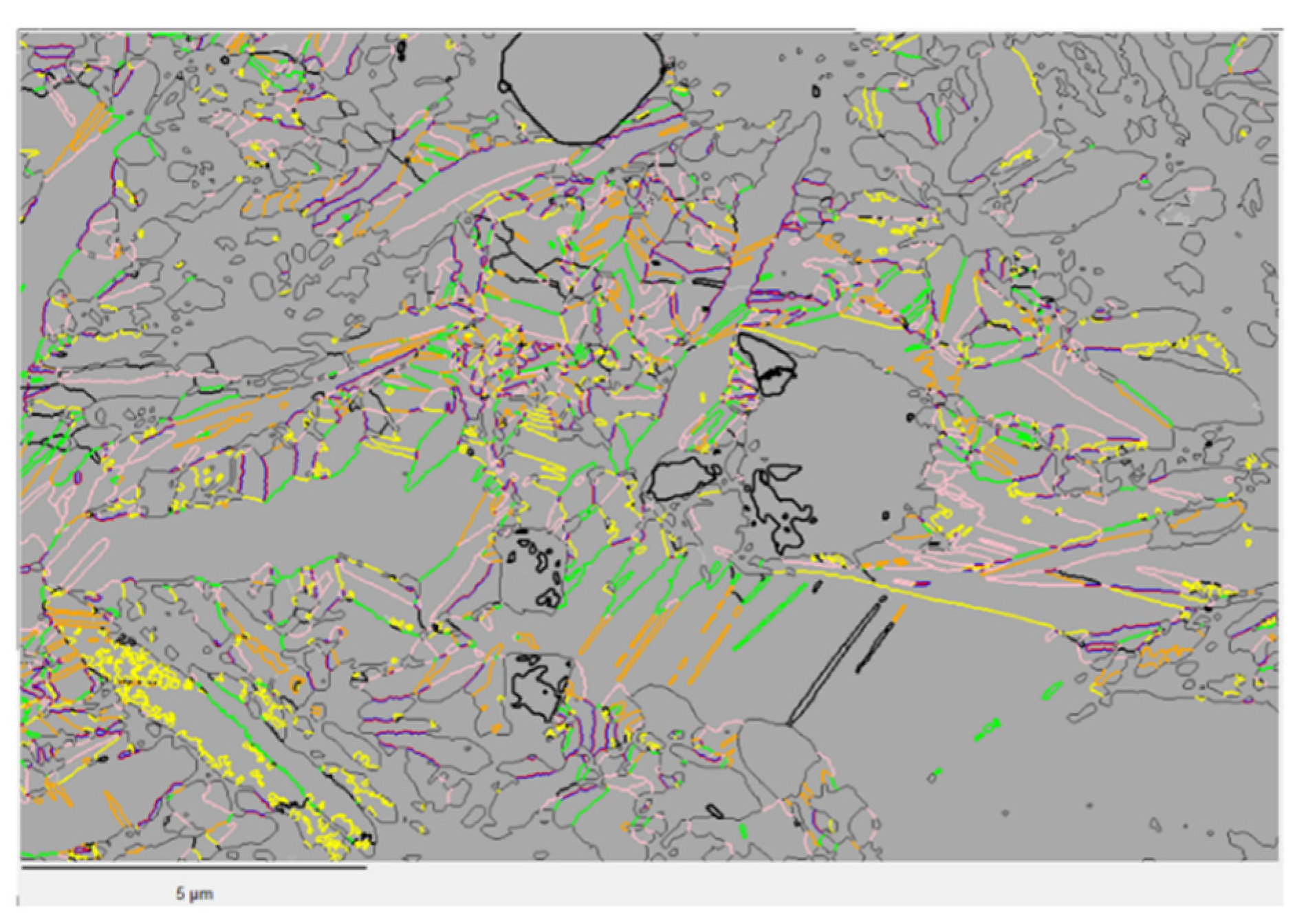
Figure A2.
TKD map of a fully martensitic B19′ NiTi alloy with the junction boundaries colored as function of the operators, such as in Figure 5.
Figure A2.
TKD map of a fully martensitic B19′ NiTi alloy with the junction boundaries colored as function of the operators, such as in Figure 5.

References
- Buehler, W.J.; Gilfrich, J.W.; Wiley, R.C. Effect of Low-Temperature Phase Changes on the Mechanical Properties of Alloys near Composition TiNi. J. Appl. Phys. 1963, 34, 1473–1477. [Google Scholar] [CrossRef]
- Bhattacharya, K. Microstructure of Martensite. In Why It Forms and How It Gives Rise to the Shape-Memory Effect, 1st ed.; Oxford University Press: New York, NY, USA, 2003. [Google Scholar]
- Otsuka, K.; Ren, X. Physical metallurgy of Ti-Ni-based shape memory alloys. Prog. Mat. Sci. 2005, 50, 511–678. [Google Scholar] [CrossRef]
- Chowdhury, P.; Sehitoglu, H. Deformation physics of shape memory alloys—Fundamentals at atomistic frontier. Prog. Mater. Sci. 2017, 88, 49–88. [Google Scholar] [CrossRef]
- Otsuka, K.; Sawamura, T.; Shimizu, K. Crystal structure and internal defects of equiatomic TiNi martensite. Phys. Stat. Sol. 1971, 5, 457–470. [Google Scholar] [CrossRef]
- Knowles, K.M.; Smith, D.A. The crystallography of the martensitic transformation in equiatomic nickel-titanium. Acta Metall. 1981, 29, 101–110. [Google Scholar] [CrossRef]
- Nishida, M.; Nishiura, T.; Kawano, H.; Inamura, T. Self-accommodation of B19’ martensite in Ti-Ni shape memory alloys-Part I. Morphological and crystallographic studies of the variant selection rules. Philos. Mag. 2012, 92, 2215–2223. [Google Scholar] [CrossRef]
- Nishida, M.; Okunishi, E.; Nishiura, T.; Kawano, H.; Inamura, T.; Li, S.; Hara, T. Self-accommodation of B19’ martensite in Ti-Ni shape memory alloys-Part II. Characteristic interface structures between habit plane variants. Philos. Mag. 2012, 92, 2234–2246. [Google Scholar] [CrossRef]
- Šittner, P.; Molnárová, O.; Kadeřávek, L.; Tyc, O.; Heller, L. Deformation twinning in martensite affecting functional behavior of NiTi shape memory alloys. Materialia 2020, 9, 100506. [Google Scholar] [CrossRef]
- Waitz, T. The self-accommodated morphology of martensite in nanocrystalline NiTi shape memory alloys. Acta Mater. 2005, 53, 2273–2283. [Google Scholar] [CrossRef]
- Liu, Y.; Xie, Z.L. Twinning and detwinning of <011> type II twin in shape memory alloy. Acta Mater. 2003, 51, 5529–5543. [Google Scholar] [CrossRef]
- Liu, Y.; Xie, Z.L. The rational Nature of Type II Twin in NiTi Shape Memory Alloy. J. Intell. Mater. Struct. 2006, 17, 1083–1090. [Google Scholar] [CrossRef]
- Ye, J.; Mishra, R.K.; Pelton, A.R.; Minor, A.M. Direct observation of the NiTi martensitic phase transformation in nanoscale volumes. Acta Mater. 2010, 58, 490–498. [Google Scholar] [CrossRef]
- Ii, S.; Yamauchi, K.; Maruhashi, Y.; Nishida, M. Direct evidence of correlation between {20-1}B19′ and {114}B2 deformation twins in Ti–Ni shape memory alloy. Scr. Mater. 2003, 49, 723–727. [Google Scholar] [CrossRef]
- Šittner, P.; Sedlák, P.; Seiner, H.; Sedmák, P.; Pilch, J.; Delville, R.; Heller, L.; Kadeřávek, L. On the coupling between martensitic transformation and plasticity in NiTi: Experiments and continuum based modelling. Prog. Mater. Sci. 2018, 98, 249–298. [Google Scholar] [CrossRef]
- Laplanche, G.; Birk, T.; Schneider, S.; Frenzel, J.; Eggeler, G. Effect of temperature and texture on the reorientation of martensite variants in NiTi shape memory alloys. Acta Mater. 2017, 127, 143–152. [Google Scholar] [CrossRef]
- Xiao, Y.; Zeng, P.; Lei, L.; Zhang, Y. In situ observation on temperature dependence of martensitic transformation and plastic deformation in superelastic NiTi shape memory alloy. Mater. Des. 2017, 134, 111–120. [Google Scholar] [CrossRef]
- Hsu, W.-N.; Polatidis, E.; Šmíd, M.; Casati, N.; Van Petegem, S.; Van Swygenhoven, H. Load path change on superelastic NiTi alloys: In situ synchrotron XRD and SEM DIC. Acta Mater. 2018, 144, 874–883. [Google Scholar] [CrossRef]
- Hsu, W.-N.; Polatidis, E.; Šmíd, M.; Van Petegem, S.; Casati, N.; Van Swygenhoven, H. Deformation and degradation of superelastic NiTi under multiaxial loading. Acta Mater. 2019, 167, 149–158. [Google Scholar] [CrossRef]
- Polatidis, E.; Šmíd, M.; Kuběna, I.; Hsu, W.-N.; Laplanche, G.; Van Swygenhoven, H. Deformation mechanisms in a superelastic NiTi alloy: An in-situ high resolution digital image correlation study. Mater. Des. 2020, 191, 108622. [Google Scholar] [CrossRef]
- Keller, R.R.; Geiss, R.H. Transmission EBSD from 10 nm domains in a scanning electron microscope. J. Microsc. 2012, 245, 245–251. [Google Scholar] [CrossRef]
- Trimby, T. Orientation mapping of nanostructured materials using transmission Kikuchi diffraction in the scanning electron microscope. Ultramicrosc 2012, 120, 16–24. [Google Scholar] [CrossRef] [PubMed]
- Suzuki, S. Feature of Transmission EBSD and its application. JOM 2013, 65, 1254–1263. [Google Scholar] [CrossRef] [Green Version]
- Cayron, C. What EBSD and TKD tell us about the crystallography of the martensitic B2-B19′ transformation in NiTi shape memory alloys. Crystals 2020, 10, 562. [Google Scholar] [CrossRef]
- Bowles, J.S.; Mackenzie, J.K. The crystallography of martensitic transformations I. Acta Metall. 1954, 2, 129–137. [Google Scholar] [CrossRef]
- Bowles, J.S.; Mackenzie, J.K. The crystallography of martensitic transformations II. Acta Metall. 1954, 2, 138–147. [Google Scholar] [CrossRef]
- Wechsler, M.S.; Liebermann, D.S.; Read, T.A. On the theory of the formation of martensite. Trans. AIME 1953, 197, 1503–1515. [Google Scholar]
- Christian, J. Applications of the phenomenological theories of martensite I–II. J. Inst. Met. 1956, 84, 386–394. [Google Scholar]
- Bain, E.C.; Dunkirk, N. The nature of martensite. Trans. AIME 1924, 70, 25–47. [Google Scholar]
- Bhadeshia, H.K.D.H. Worked Examples in the Geometry of Crystals, 2nd ed.; The Institute of Metals: London, UK, 1987. [Google Scholar]
- Wayman, C.M. Shear transformations and microstructures. Metallography 1975, 8, 105–130, republished in Mater. Charact. 1997, 39, 235–260. [Google Scholar] [CrossRef]
- Duparc, O.B.M.H. A review of some elements for the history of mechanical twinning centred on its German origins until Otto Mügge’s K1 and K2 invariant plane notation. J. Mater. Sci. 2016, 52, 4182–4196. [Google Scholar] [CrossRef]
- Mügge, O. Ueber Homogene Deformationen (einfache Schiebungen) an den Triklinen Doppelsalzen BaCdCl4.4aq., Neues Jahrbuch für Mineralogie, Geologie und Palaeontologie Beilage-Band. 1889. Available online: https://www.phase-trans.msm.cam.ac.uk/2001/geometry2/Geometry.pdf (accessed on 22 November 2021).
- Kihô, H. The Crystallographic Aspect of the Mechanical Twinning in Metals. J. Phys. Soc. Jpn. 1954, 9, 739–747. [Google Scholar] [CrossRef]
- Jaswon, M.A.; Dove, D.B. The Crystallography of Deformation Twinning. Acta Cryst. 1960, 13, 232–240. [Google Scholar] [CrossRef] [Green Version]
- Bilby, B.A.; Crocker, A.G. The Theory of the Crystallography of Deformation Twinning. Proc. R. Soc. Lond. Ser. A 1965, 288, 240–255. [Google Scholar]
- Bevis, M.; Crocker, A.G. Twinning Shears in Lattices. Proc. R. Soc. Lond. Ser. A 1968, 304, 123–134. [Google Scholar]
- Cahn, R.W. Twinned Crystals. Adv. Phys. 1954, 3, 363–445. [Google Scholar] [CrossRef]
- Christian, J.W.; Mahajan, S. Deformation Twinning. Prog. Mater. Sci. 1995, 39, 1–157. [Google Scholar] [CrossRef]
- Gupta, S.P.; Johnson, A.A. Morphology and crystallography of beta’ martensite in TiNi alloys. Trans. Jpn. Inst. Metals. 1973, 14, 292–302. [Google Scholar] [CrossRef] [Green Version]
- Sinclair, R. Origin of stacking faults in NiTi martensite. AIP Conf. 1979, 53, 269. [Google Scholar]
- Nishida, M.; Yamauchi, K.; Itai, I.; Ohgi, H.; Chiba, A. High resolution electron microscopy studies of twin boundary structure in B19’ martensite in the Ti-Ni shape memory alloy. Acta Metall. Mater. 1995, 43, 1229–1234. [Google Scholar] [CrossRef]
- Mohammed, A.S.K.; Sehitoglu, H. Modeling the interface structure of type II boundary in B19’ NiTi from an atomistic and topological standpoint. Acta Mater. 2020, 183, 93–109. [Google Scholar] [CrossRef]
- Miyazaki, S.; Kimura, S.; Otsuka, K.; Suzuki, Y. The habit plane and transformation strains associated with martensitic transformation in Ti-Ni single crystals. Scr. Metall. 1984, 18, 883–888. [Google Scholar] [CrossRef]
- Miyazaki, S.; Otsuka, K.; Wayman, C.M. The shape memory mechanism associated with the martensitic transformation in Ti-Ni alloys-I. Self-accommodation. Acta Metall. 1989, 37, 1873–1884. [Google Scholar] [CrossRef]
- Ball, J.M.; James, R.D. Finite phase mixtures as minimizers of energy. Arch. Ration. Mech. Anal. 1987, 100, 13–52. [Google Scholar] [CrossRef]
- Pitteri, M.; Zanzotto, G. Generic and non-generic cubic-to-monoclinic transitions and their twins. Acta Mater. 1998, 46, 225–237. [Google Scholar] [CrossRef]
- Pitteri, M.; Zanzotto, G. Continuum Models for Phase Transitions and Twinning in Crystals; Chapman & Hall/CRC: Boca Raton, FL, USA, 2003. [Google Scholar]
- Hane, K.F.; Shield, T.W. Microstructure in the cubic to monoclinic transition in titanium-nickel shape memory alloys. Acta Mater. 1999, 47, 2603–2617. [Google Scholar] [CrossRef]
- Inamura, T.; Nishiura, T.; Kawano, H.; Hosoda, H.; Nishida, M. Self-accommodation of B19’ martensite in Ti-Ni shape memory alloys-Part III. Analysis of habit plane variant clusters by the geometrically nonlinear theory. Philos. Mag. 2012, 92, 2247–2263. [Google Scholar] [CrossRef]
- Gu, H.; Bumke, L.; Chluba, C.; Quandt, E.; James, R.D. Phase engineering and supercompatibility of shape memory alloys. Mater. Todays 2018, 21, 265–277. [Google Scholar] [CrossRef]
- Song, Y.; Chen, X.; Dabade, V.; Shield, T.W.; James, R.D. Enhanced reversibility and unusual microstructure of a phase-transforming material. Nature 2013, 502, 85–88. [Google Scholar] [CrossRef]
- Chen, X.; Liu, T.; Li, R.; Liu, J.; Zhao, Y. Molecular dynamics simulation on the shape memory effect and superelasticity in NiTi shape memory alloy. Comput. Mater. Sci. 2018, 146, 61–69. [Google Scholar] [CrossRef]
- Li, B.; Shen, Y.; An, Q. Structural origin of reversible martensitic transformation and reversible twinning in NiTi shape memory alloy. Acta Mater. 2020, 199, 240–252. [Google Scholar] [CrossRef]
- Janovec, V. Group analysis of domains and domain pairs. Czech. J. Phys. B 1972, 22, 975–994. [Google Scholar] [CrossRef]
- Janovec, V.; Hahn, T.; Klapper, H. International Tables for Crystallography; Authier, A., Ed.; Kluwer Academic Publishers: Dordrecht, The Netherlands, 2003; Volume D, pp. 377–391. [Google Scholar]
- Cayron, C. Groupoid of orientational variants. Acta Cryst. 2006, 62, 21–40. [Google Scholar] [CrossRef] [Green Version]
- Cayron, C. GenOVa: A computer program to generate orientational variants. J. Appl. Cryst. 2007, 40, 1179–1182. [Google Scholar] [CrossRef] [Green Version]
- Cayron, C. ARPGE: A computer program to automatically reconstruct the parent grains from electron backscatter diffraction data. J. Appl. Cryst. 2007, 40, 1183–1188. [Google Scholar] [CrossRef] [Green Version]
- Cayron, C.; Barcelo, F.; de Carlan, Y. The mechanisms of the fcc–bcc martensitic transformation revealed by pole figures. Acta Mater. 2010, 58, 1395–1402. [Google Scholar] [CrossRef]
- Cayron, C. One-step model of the face-centred-cubic to body-centred-cubic martensitic transformation. Acta Cryst. 2013, 69, 498–509. [Google Scholar] [CrossRef]
- Cayron, C. Continuous atomic displacements and lattice distortion during fcc–bcc martensitic transformation. Acta Mater. 2015, 96, 189–202. [Google Scholar] [CrossRef] [Green Version]
- Cayron, C. Angular distortive matrices of phase transitions in the fcc-bcc-hcp system. Acta Mater. 2016, 111, 417–441. [Google Scholar] [CrossRef] [Green Version]
- Baur, A.P.; Cayron, C.; Logé, R. {225}γ habit planes in martensitic steels: From the PTMC to a continuous model. Sci. Rep. 2017, 7, 40938. [Google Scholar] [CrossRef] [PubMed]
- Baur, A.P.; Cayron, C.; Logé, R. Variant selection in surface martensite. J. Appl. Cryst. 2017, 50, 1646–1652. [Google Scholar] [CrossRef] [Green Version]
- Baur, A.P.; Cayron, C.; Logé, R. Variant selection in Fe-2Ni-1.8C under bending. Crystals 2018, 8, 474. [Google Scholar] [CrossRef] [Green Version]
- Larcher, M.N.D.; Cayron, C.; Blatter, A.; Soulignac, R.; Logé, R. EBSD Study of Variant Selection during Ordering Phase Transformation in L10-type Red Gold Alloy. J. Appl. Cryst. 2019, 52, 1202–1213. [Google Scholar] [CrossRef]
- Larcher, M.N.D.; Cayron, C.; Blatter, A.; Soulignac, R.; Logé, R. The thermally activated distortion with amplification effect and related variant selection in red gold alloys. Acta Mater. 2020, 198, 242–256. [Google Scholar] [CrossRef]
- Cayron, C. The transformation matrices (Distortion, orientation, correspondence), their continuous forms and their variants. Acta Cryst. 2019, 75, 411–437. [Google Scholar]
- Jaswon, M.A.; Wheeler, J.A. Atomic Displacements in the Austenite-Martensite Transformation. Acta Cryst. 1948, 1, 216–224. [Google Scholar] [CrossRef]
- Cayron, C. Complements to Mügge and Friedel’s theory of twinning. Metals 2020, 10, 231. [Google Scholar] [CrossRef] [Green Version]
- Cayron, C.; Logé, R. Evidence of new twinning modes in magnesium questioning the shear paradigm. J. Appl. Cryst. 2018, 51, 809–817. [Google Scholar] [CrossRef] [Green Version]
- Cayron, C. Shifting the shear paradigm in the crystallographic models of displacive transformations in metals and alloys. Crystals 2018, 8, 181. [Google Scholar] [CrossRef] [Green Version]
- Cayron, C. The weak plane and weak twins. in preparation.
- Cayron, C. Hard-sphere displacive model of extension twinning in magnesium. Mater. Des. 2017, 119, 361–375. [Google Scholar] [CrossRef] [Green Version]
- Christian, J.W. Deformation by Moving Interfaces. Metall. Trans. A 1982, 13, 509–538. [Google Scholar] [CrossRef]
Figure 1.
A 2D example of a square austenite (A) → parallelogram martensite (M) transformation. (a) There are four orientation variants, assuming for the “natural” OR. (b) Closing-gap OR and associated rotation gradients between the variants and . This new OR maintains invariant the vertical reflection plane . (c) Closing-gap OR and associated rotation gradients between the variants and . This new OR maintains invariant the diagonal reflection plane . (d) Global compatibility between the variants mediated by the closing-gap ORs and associated orientation gradients.

Figure 2.
Junction plane between variants and deduced from the austenite symmetry operation that links them. (a) Reflection on the austenite plane , and (b) 180° rotation around the austenite axis .
Figure 2.
Junction plane between variants and deduced from the austenite symmetry operation that links them. (a) Reflection on the austenite plane , and (b) 180° rotation around the austenite axis .
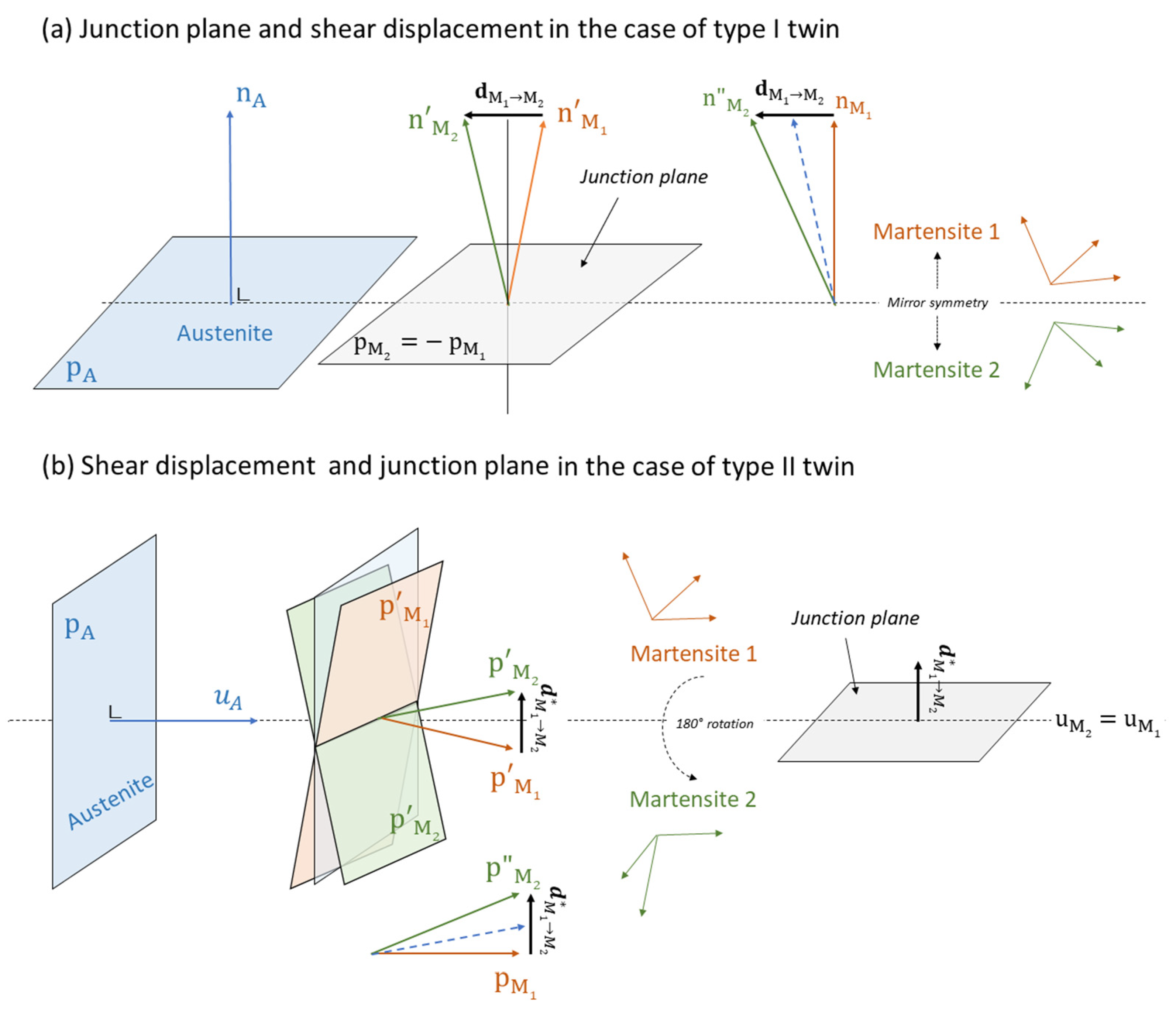
Figure 3.
Axial weak plane between two crystals: 1 and 2. (a) The rational directions and are the same vector; it is the invariant axis of the twin. The rational directions and have close norms and make nearly the same angle with the axis of the twin. The weak plane is parallel to ; it is the plane of the page; its Miller indices are the coordinates of the reciprocal vector in the crystallographic basis of crystal 1 , and of in . (b) The slight intraplanar distortion represented by the black arrows transforms into .
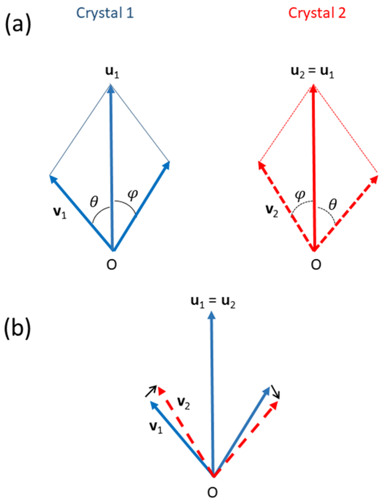
Figure 4.
Theoretical disorientation histogram and rotation axes built from all the orientation variants of all the closing-gap ORs presented in Table 4.
Figure 4.
Theoretical disorientation histogram and rotation axes built from all the orientation variants of all the closing-gap ORs presented in Table 4.
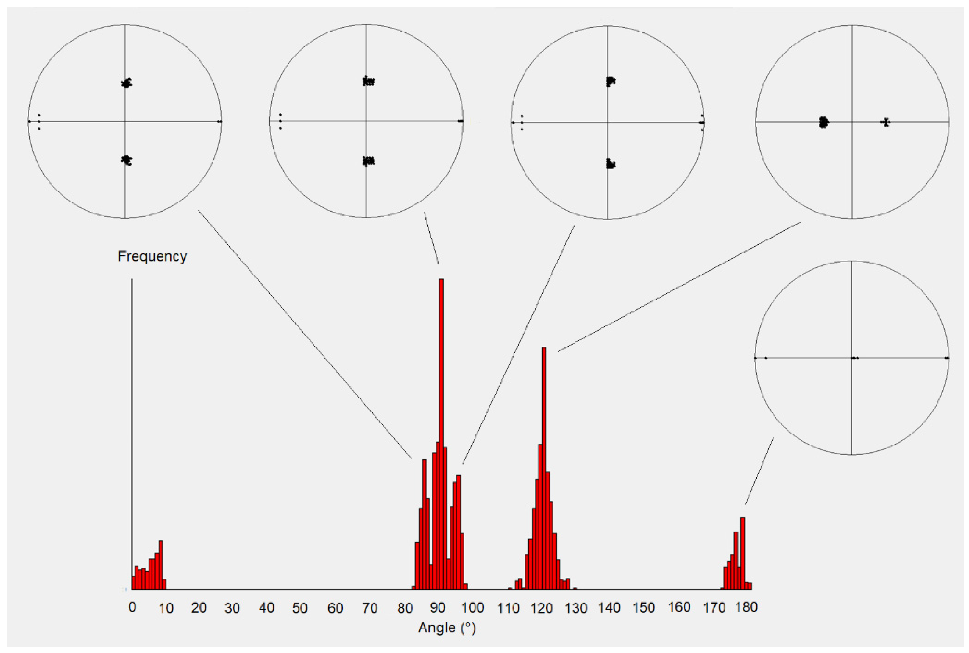
Figure 5.
TKD map of a B19′ martensitic NiTi alloy. (a) IPF-Y colored map of the B19′ grains. (b) Specific grain boundaries colored in a TKD map according to the operators. The polar operators and in red and blue, respectively, overlap on each side of the grain boundaries and merge into a purple color.
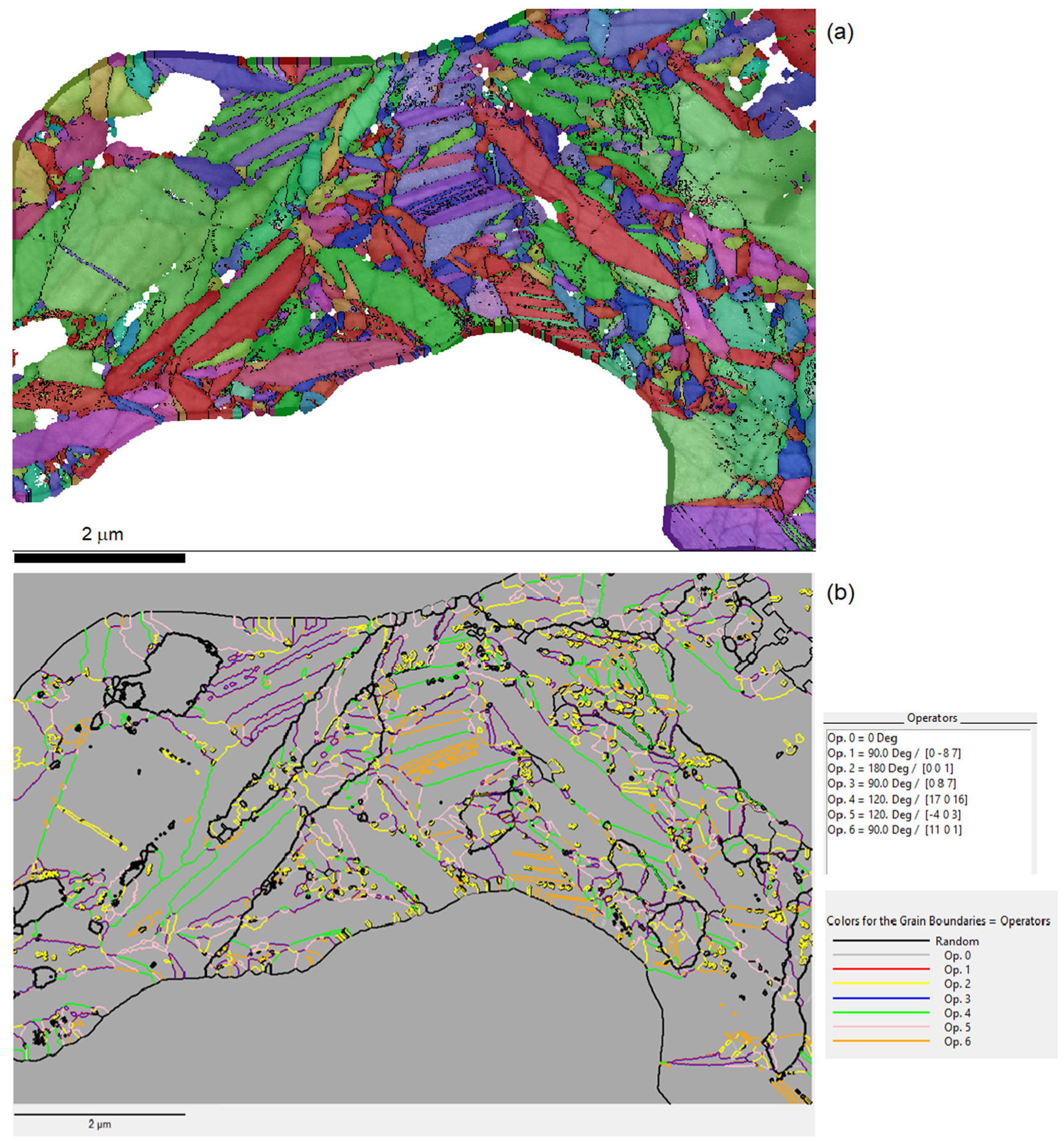
Figure 6.
Traces of the junction planes predicted by the CT for the operators (a) , (b) , (c) , (d) (e) and . The comparison for each pair of B19′ variants is visually made by considering whether the traces are parallel to the grain boundaries. Good agreement was found for most of the boundaries that were considered.
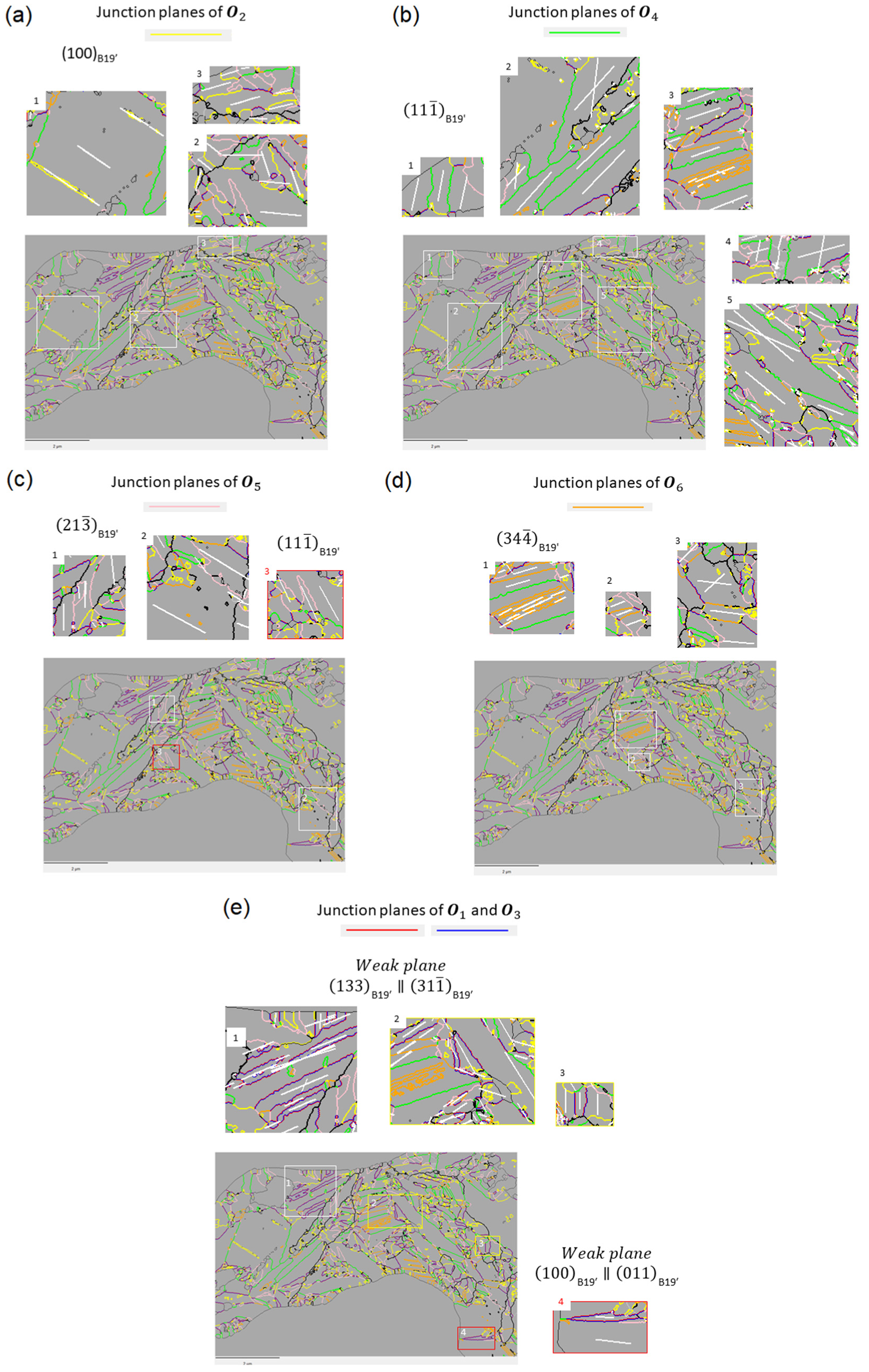
Figure 7.
B19′ martensite reorientated by bending a martensitic NiTi bar (10 mm long and 2 mm thick) at room temperature into a U-shape. (a) IPF-X EBSD map of the B19′ phase. The map was acquired in the tensile part, with the tensile direction along X (horizontal direction). The initial microstructure before bending was constituted of long lenticular laths (see Figure 4b of Ref. [24]). The reddish color of the IPF-X map and the high density close to in the IPF map presented on the right-hand side (Multiple of Uniform Distribution, MUD = 27) show that the B19′ variants are reorientated under the stress. (b) IPF-X map of the parent B2 grains reconstructed with ARPGE.
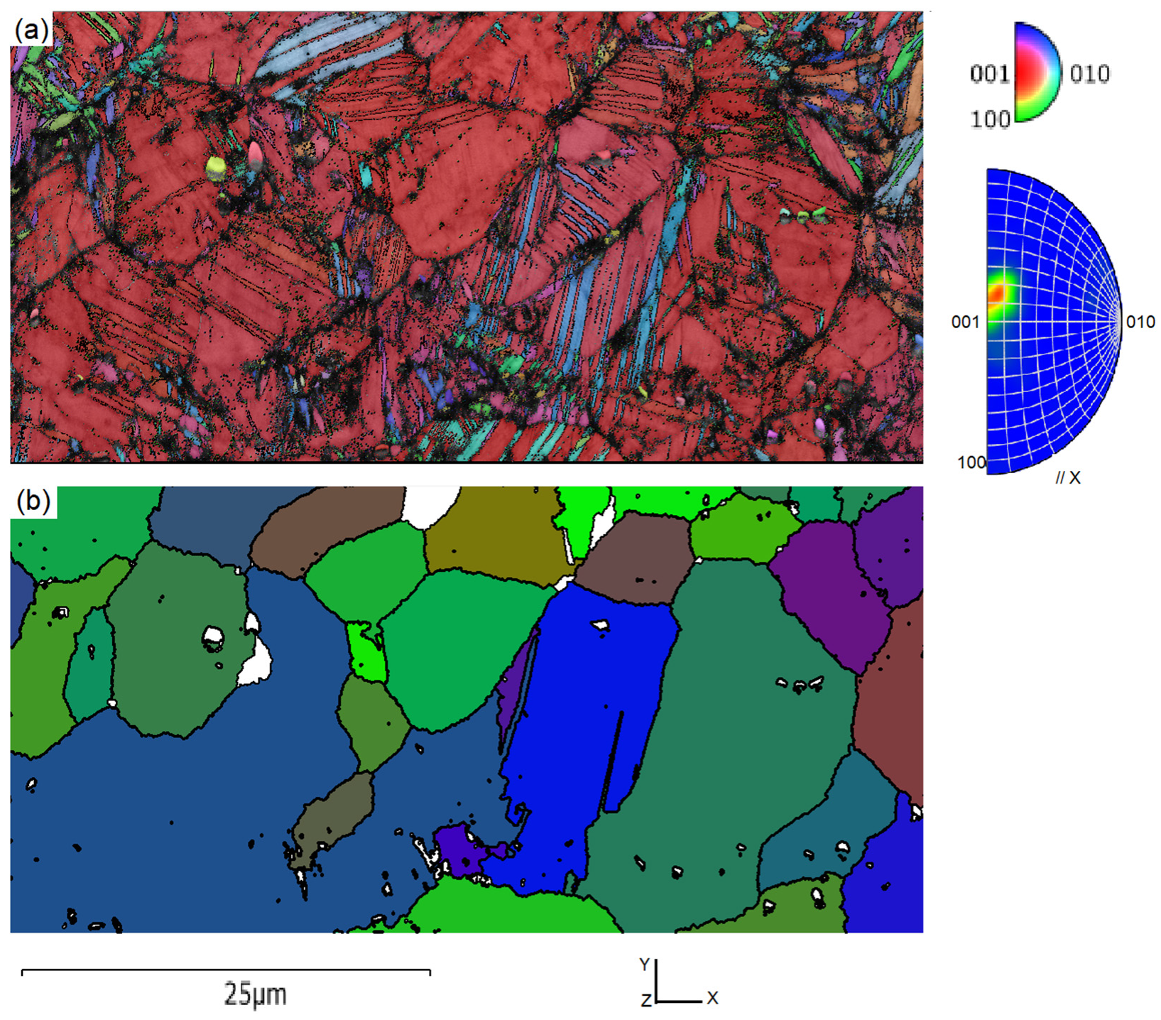
Table 1.
Intersection subgroup, variants and operators of the B2 → B19′ transformation for correspondence, orientation and distortion relations. For this transformation, the intersection subgroup does not depend on the type of relation, and is just noted as .
Table 1.
Intersection subgroup, variants and operators of the B2 → B19′ transformation for correspondence, orientation and distortion relations. For this transformation, the intersection subgroup does not depend on the type of relation, and is just noted as .
| Correspondence | Orientation | Distortion |
|---|---|---|
| Intersection subgroups | ||
| Variants (from simple cosets) | ||
| Number of variants (Lagrange’s formula) | ||
| 12 | 12 | 12 |
| Operators (from double cosets) | ||
| Number of operators (Burnside’s formula) | ||
| 7 | 7 | 7 |
Table 2.
List of operators for the B2 → B19′ transformation. The operators are numbered from 0 (identity operator) to 6; the order results from the double-coset decomposition made in GenOVa. The operators are classified here into three categories: the neutral operator ; the ambivalent operators and the complementary polar operators . The second column gives the disorientation, i.e., the smallest rotation in the set . The third and fourth columns give the B2 symmetries in the double cosets by their matrices and by symmetry elements, respectively. The elements in bold are two-fold symmetries.
| B2 Symmetries in the Double Cosets | |||
|---|---|---|---|
| Disorient. | Matrices | Geometrical Elements | |
| , , , | |||
| , , , | |||
| , , | |||
| , , , | |||
| , , , | |||
| , , , | |||
| , , , | |||
| , | |||
| , , , | |||
| , , , | |||
| , , | |||
| , , , | |||
Table 3.
Junction planes and twin characteristics predicted by the inter-correspondence operator between the B19′ variants. We indicate, for the type I twins, the B2 reflection plane and the B19′ twin plane (junction plane) and, for the type II twins, the B2 180° axis and the B19′ twin axis. The invariant but irrational plane K2 is written by a rational approximate tagged by a symbol . The arrows mean both “correspondence” and “parallelism”. The junction planes that agree with the observations (Section 5.4) are written in bold.
| Reflection Junction Plane (Type I) | Rotational Junction Plane (Type II and Weak) | Shear Amplitude | |
|---|---|---|---|
| or | s = 0.2389 | ||
| s = 0.3096 | |||
| s = 0.1422 | |||
| s = 0.2804 | |||
| no solution | sg = 0.2911 | ||
Table 4.
Closing-gap ORs between two B19′ variants linked by the operator predicted by the correspondence theory. In the last column are the deviation angles between the closing-gap OR and the natural OR AQ [24]. For each operator, the minimum angle is written in bold.
Table 4.
Closing-gap ORs between two B19′ variants linked by the operator predicted by the correspondence theory. In the last column are the deviation angles between the closing-gap OR and the natural OR AQ [24]. For each operator, the minimum angle is written in bold.
| Op. | OR | Deviation from AQ OR |
|---|---|---|
| 1.43° | ||
| 8.23° | ||
| )B2 and | 2.21° | |
| and | 8.88° | |
| )B2 and | 8.11° | |
| and | 2.15° | |
| )B2 and | 7.93° | |
| and | 3.94° | |
| case 1: | 7.04° | |
| case 2: and | 3.45° |
Table 5.
Comparison between the CT and the PTMC to predict the B19′ junction planes associated with the operators . The letters t.I, t.II and C mean “type I”, “type II” and “compound” twins, respectively. In the column “Name in PTMC”, notation with the letter “S” was used by Hane and Shield [51] and notation with a letter (A, B, etc.) by Bhattacharya [2]. For the correspondence theory, the letter W means “weak twin”. The junction planes experimentally observed are written in bold.
| Closing-Gap Disorientation | Junction Planes CT | Shear | Junction Planes PTMC | Name in PTMC | Shear | |
|---|---|---|---|---|---|---|
(from C1) | C1: , C2: | 0.2385 | C1: , C2: | S1, A | 0.2385 | |
(from I) | t.I: t.II: W: | 0.3096 | t.I: t.II: | S3, D/C | 0.3096 | |
(from W) | t.I: t.II: W: | 0.1422 | t.I: t.II: | S4, C/D | 0.1423 | |
(from W) | t.I: t.II: W: | 0.2804 | t.I: t.II: | S2, B | 0.2804 | |
| W: | 0.2912 | no solution | S5 | no value | ||
| S6 |
Publisher’s Note: MDPI stays neutral with regard to jurisdictional claims in published maps and institutional affiliations. |
© 2022 by the author. Licensee MDPI, Basel, Switzerland. This article is an open access article distributed under the terms and conditions of the Creative Commons Attribution (CC BY) license (https://creativecommons.org/licenses/by/4.0/).
Share and Cite
MDPI and ACS Style
Cayron, C. The Correspondence Theory and Its Application to NiTi Shape Memory Alloys. Crystals 2022, 12, 130. https://doi.org/10.3390/cryst12020130
AMA Style
Cayron C. The Correspondence Theory and Its Application to NiTi Shape Memory Alloys. Crystals. 2022; 12(2):130. https://doi.org/10.3390/cryst12020130
Chicago/Turabian StyleCayron, Cyril. 2022. "The Correspondence Theory and Its Application to NiTi Shape Memory Alloys" Crystals 12, no. 2: 130. https://doi.org/10.3390/cryst12020130
Note that from the first issue of 2016, this journal uses article numbers instead of page numbers. See further details here.