Explore Optical Solitary Wave Solutions of the kp Equation by Recent Approaches

Abstract

The study of nonlinear evolution equations is a subject of active interest in different fields including physics, chemistry, and engineering. The exact solutions to nonlinear evolution equations provide insightful details and physical descriptions into many problems of interest that govern the real world. The Kadomtsev–Petviashvili (kp) equation, which has been widely used as a model to describe the nonlinear wave and the dynamics of soliton in the field of plasma physics and fluid dynamics, is discussed in this article in order to obtain solitary solutions and explore their physical properties. We obtain several new optical traveling wave solutions in the form of trigonometric, hyperbolic, and rational functions using two separate direct methods: the $(w/g)$-expansion approach and the Addendum to Kudryashov method (akm). The nonlinear partial differential equation (nlpde) is reduced into an ordinary differential equation (ode) via a wave transformation. The derived optical solutions are graphically illustrated using Maple 15 software for specific parameter values. The traveling wave solutions discovered in this work can be viewed as an example of solutions that can empower us with great flexibility in the systematic analysis and explanation of complex phenomena that arise in a variety of problems, including protein chemistry, fluid mechanics, plasma physics, optical fibers, and shallow water wave propagation.

1. Introduction

In physical science, the study of traveling wave solutions is critical for understanding and quantitatively describing a variety of nonlinear phenomena. In most cases, complex phenomena in nature generally involve nonlinear properties that can be characterized by nlpdes where solitary and soliton solutions may appear [1,2]. Nonlinear chaotic systems, plasma waves, heat conduction systems, diffusion processes, ocean engineering, and chemical physics, for example, are modeled and described by nonlinear equations [3,4,5]. Therefore, it is significant to investigate exact traveling wave solutions, since new exact solutions may provide a better understanding of most physical and biological phenomena that these models represent. Furthermore, exact solutions can enable us to explore the stability of desired solutions as well as to perform numerical analysis for nlpdes. Solitary and soliton waves solutions which are solutions of specific nlpdes are considered to be a special classes of traveling wave solutions that have distinct features. These distinct features can determine the behavior of the solution, and hence the properties of the phenomena with which the nlpde is formed [6]. The solitary waves consist of a sequence of solitary waves that propagate without changing shape or size over time. Such solitary waves have been observed in many science and engineering applications, such as surface water elevation and light intensity in optical fibers. Soliton, on the other hand, is a nonlinear solitary wave that provides vital insights into the dynamics of solitary waves and also forms a particular class of Korteweg–de-Vries (kdv) solutions. Solitons have attracted interest from researchers after Gardner et al. [7] developed the inverse scattering method for solving the kdv equations.

Despite the tremendous successes of nlpdes in characterizing the complex phenomena, not all of the models’ equations are solvable. Hence, familiarity with all classic and recently established approaches for addressing these models becomes increasingly vital. Over the past few years, numerous strategies have been proposed by mathematicians and scientists, such as the F-expansion method [8], the variational iteration method [9], method of sine–cosine [10], the tanh-function technique [11], the auxiliary equation method [12], the exp-function technique [13,14], the exact soliton solution [15,16,17], the generalized Kudryashov approach [18], and the newly extended generalized Kudryashov approach [19]. A more detailed discussion on some recent direct methods can be found in several related works (see, for example, [20,21,22,23]).

The kdv is a nonlinear partial differential equation which has a fundamental role in describing the dynamics of long waves in acoustic waves on a crystal lattice, shallow water waves, optics and plasma physic, quantum mechanics, and fluid mechanics. The kdv equation is expressed in the form [24]:

$$u_t+u_{xxx}+6u_x{u}_{xx}=0,$$

here, x and t denote respectively the independent spatial and time variables; $u=u(x,y,t)$ and $u_t=\partial u/\partial t, u_x=\partial u/\partial x$ and so on. This equation was used to describe how waves arise under the influence of weak nonlinearity of $u_x{u}_{xx}$ and linear dispersion of $u_{xxx}$. In addition, it is broadly applied in many science and engineering applications to describe weakly nonlinear long waves [1,25,26].

In the 1970s, Kadomtsov and Petviashivili introduced a two-dimensional dispersive wave equation, known as kp equation, as an extension of the nonlinear $(1+1)$ dimensional kdv equation. This equation aims to study nonlinear waves varying slowly in a dispersive medium under the influence of weak transversal perturbations. Here, as an application of the $(w/g)$-expansion approach and the akm, we study the kp equation to explore the new traveling wave solutions. For the purposes of discussion, consider the dependent variable $u=u(x,y,t)$ satisfying the $(2+1)$-dimensional kp equation [27]:

$$u_{xt}-6u{u}_{xx}-6{\left(u_x\right)}^2+u_{xxxx}+3{\delta }^2{u}_{yy}=0,$$

(1)

or

$$\begin{array}{c}\hfill {(u_t-6u{u}_x+u_{xxx})}_x+3{\delta }^2{u}_{yy}=0,\end{array}$$

where the independent spatial variables are x and y, and the time variable is t. Assuming that ${\delta }^2=1$, then the system (1) is used to analyze weakly nonlinear dispersive waves in plasma as well as weakly nonlinear long water waves in modulation. However, setting ${\delta }^2=1$, then the system (1) is used to study acoustic waves and admits unstable soliton solutions.

In recent years, the investigation of exact traveling wave solutions of the kp model is becoming successively attractive to many researchers due to its great applications in various fields, especially in the field of fluid dynamics and plasma physics. For example, Khan and Akbar [27] explored the traveling wave solutions of the kp equation employing method of the $exp(-\Phi (\xi \left)\right)$-expansion. Chen [28] investigated $(3+1)$-dimensional kp equation by implementing the new generalized transformation in the homogeneous balance method. Other methods that have been successively applied to construct an exact solution from this model include a modified simple equation method [29], decomposition method [30], Hirota’s bilinear method and the tanh-coth method [31], and the generalized expansion method [32].

Wen-An et al. [33] explored the modified $(w/g)$-expansion approach for constructing wave solutions of the Vakhnenko equation which is applied to describe the high-frequency wave propagation in relaxing media. This expansion approach is considered as the generalization of the $(G^{\prime }/G)$-expansion method, which was introduced by Wang et al. [34]. For certain special choices of the function w and g, two new expansion methods can be obtained, namely, $(g^{\prime }/g^2)$-expansion and $\left(g^{\prime }\right)$-expansion. Here, we focus attention on applying these interesting new expansion methods to obtain new traveling wave solutions of kp Equation (1).

In this paper, Section 2 describes briefly the procedure of the modified ($w/g$)-expansion method. Section 3 presents the three expansion methods; namely, the modified $(g^{\prime }/g^2)$-expansion approach and $\left(g^{\prime }\right)$-expansion approach, and the generalized simple $(w/g)$-expansion approach. The akm is introduced and applied, in Section 4, to obtain new optical solitary wave solutions of the kp equation. The results of this study are graphically described in Section 5 using the Maple 15 program. Although this article focuses on exploring the exact traveling solutions of the kp equation, we expect that the presented direct expansions methods should also be able to investigate a wide range of nonlinear problems in mathematical physics and engineering applications.

2. Methodology of the Modified (w/g)-Expansion Approach

This section describes briefly the basic idea of the modified ($w/g$)-expansion approach as presented in [33,35]. We assume that a general nlpde in two variables x and t is given by:

$$P(u,u_t,u_x,u_{tt},u_{xx},u_{xt},\dots )=0,$$

(2)

where $u(x,y,t)$ is an unidentified function and P is a polynomial function in $u=u(x,t)$ and its partial derivatives, which includes both linear and nonlinear terms. The following steps are used to solve the above nlpde:

Step 1. We seek the traveling wave transformation to convert the independent variables x and t into a compound variable $\xi$ in the following form:

$$u(x,t)=U\left(\xi \right),$$

(3)

where $\xi =x-kt$, k is the wave speed. This transformation Equation (3) empowers us to convert the nlpde (2) to the following ode:

$$Q(U,U^{\prime },U^{″},\dots )=0,$$

(4)

where Q denotes a polynomial function in $U\left(\xi \right)$ and its derivatives $U^{\prime }$ with respect to $\xi$. Since Equation (3) is a completely integrable equation, we integrate it with respect to $\xi$ to obtain $Q_1(U,U^{\prime },U^{\prime },\dots )=0$.

Step 2. Assuming that the solution to the ode (4) is given by:

$$U\left(\xi \right)=\sum _{i=0}^m{a}_i{\left(\frac{w\left(\xi \right)}{g\left(\xi \right)}\right)}^i,$$

(5)

where $a_i$ are constants, for $i=0,1,\dots ,m.$ The functions $w=w\left(\xi \right)$ and $g\left(\xi \right)$ satisfy the following ode:

$${\left(\frac{w\left(\xi \right)}{g\left(\xi \right)}\right)}^{{}^{\prime }}=a+b\left(\frac{w\left(\xi \right)}{g\left(\xi \right)}\right)+c{\left(\frac{w\left(\xi \right)}{g\left(\xi \right)}\right)}^2,$$

(6)

or

$$w^{\prime }g-w{g}^{\prime }=a{g}^2+bwg+c{w}^2,$$

(7)

where $a,b,$ and c are constants.

Step 3. By balancing the nonlinear term and the highest order derivative appearing in the ode (4), we find the positive integer n in Formula (5).

Step 4. Substitute the solution (5) into the ode (4) along with the first order Equation (6); and combine together any terms with the same powers of ${(w/g)}^i$, for $i=0,1,2,\dots ,m$, so that the left-hand side of the ode (4) is turned into a polynomial in ${(w/g)}^i$. In this polynomial, we equate all the coefficients to zero. As a result of this procedure, we get a system of equations for $a_i,$ when $i=0,1,\dots ,m,$ and $k$.

Step 5. Solve this system of equations by the assistance of Mathematica or Maple and we find $a_i,$ and k.

3. Application of Extended Rational (w/g)-Expansion Approach

This section presents three expansion methods; namely, the modified $(g^{\prime }/g^2)$-expansion approach and $\left(g^{\prime }\right)$-expansion approach, and the generalized simple $(w/g)$-expansion approach to explore new optical solitary wave solutions for nonlinear equations via kp Equation (1).

As an illustration, we consider the nonlinear kp Equation (1). The traveling wave variable given below

$$u(x,y,t)=U\left(\xi \right),\xi =x+y-kt,$$

(8)

where k is an arbitrary constant that permits us to convert the nonlinear kp Equation (1) to the following ode:

$${\left(k{U}^{\prime }-6U{U}^{\prime }+U^{‴}\right)}^{\prime }+3{\delta }^2{U}^{″}=0,$$

by integrating twice, we have:

$$U^{″}+\left(3{\delta }^2-k\right)U-3U^2+C_1=0,$$

(9)

where $C_1$ is the integration constant.

3.1. The Modified $(g^{\prime }/g^2)$-Expansion Approach

This subsection implements the modified $(g^{\prime }/g^2)$-expansion approach to the kp Equation (9) to derive new traveling wave solutions. By setting $w=g^{\prime }/g,$ and $b=0$ in the auxiliary Equation (7), we obtain new expansion so that $u\left(\xi \right)$ is given by:

$$U\left(\xi \right)=\sum _{i=0}^m{a}_i{\left(\frac{g^{\prime }}{g^2}\right)}^i,$$

(10)

where $a_i$ are constants for $i=0,1,\dots ,m$, and $g\left(\xi \right)$ satisfies the nlpde in the form

$$g^2{g}^{″}-2g{\left(g^{\prime }\right)}^2=a{g}^4+c{\left(g^{\prime }\right)}^2,$$

(11)

this is known as the $(g^{\prime }/g^2)$-expansion approach which has been introduced in [33]. Balancing the highest order derivative $U^{″}$ and the nonlinear term $U^2$ in Equation (9) using the homogeneous balance method [36] yields the degree m of the polynomial must equal to 2. As a result, the solution of Equation (9) has the following form:

$$U\left(\xi \right)=a_0+a_1\left(\frac{g^{\prime }}{g^2}\right)+a_2{\left(\frac{g^{\prime }}{g^2}\right)}^2.$$

(12)

Here, $a_0,a_1$, and $a_2$ are constants, so that, $g\left(\xi \right)$ satisfies Equation (11). Substitute Equations (11) and (12) into Equation (9) and combine together any terms with the same powers of ($g^{\prime }/g^2$). As a result of this substitution, the left-hand side of Equation (9) is reduced into a polynomial function in ($g^{\prime }/g^2$). We equate all the coefficients of this polynomial to zero. This procedure produces a system of algebraic equations for $a_0, a_1, a_2, C_1$ and k that can be addressed by using Mathematica or Maple to obtain:

$$a_0=\frac{4}{3}ac+\frac{1}{2}{\delta }^2-\frac{1}{6}k,a_1=0,a_2=2c^2,C_1=\frac{4}{3}{c}^2{a}^2-\frac{3}{4}{\delta }^4+\frac{1}{2}{\delta }^{2}k-\frac{1}{12}{k}^2,$$

where $a, c,$ and k are constants. Therefore, the general solutions of Equation (11) take the following form:

$$g\left(\xi \right)=\left\{\begin{array}{c}\begin{array}{cc}\hfill & \frac{2c}{ln\left[\frac{c}{a}{[A_{1}sin\left(\sqrt{ac}\xi \right)-A_{2}cos\left(\sqrt{ac}\xi \right)]}^2\right]},ca>0\hfill \\ \hfill & -\frac{2c}{2\sqrt{\left|ac\right|}\xi -ln[\frac{c}{4a}{(A_1{e}^{2\sqrt{\left|ac\right|}\xi }-A_2)}^2]},ca<0\hfill \\ \hfill & \frac{c}{ln\left[A_{1}c\xi +A_{2}c\right]},a=0,c\ne 0\hfill \end{array}\end{array}\right.$$

and

$$\left(\frac{g^{\prime }}{g^2}\right)=\left\{\begin{array}{c}\begin{array}{cc}\hfill & \sqrt{\frac{a}{c}}\left[\frac{A_{1}cos\left(\sqrt{ac}\xi \right)+A_{2}sin\left(\sqrt{ac}\xi \right)}{A_{1}sin\left(\sqrt{ac}\xi \right)-A_{2}cos\left(\sqrt{ac}\xi \right)}\right],ca>0\hfill \\ \hfill & \frac{1}{2c}\left[2\sqrt{\left|ac\right|}-\frac{4\sqrt{\left|ac\right|}{A}_1{e}^{2\sqrt{\left|ac\right|}\xi }}{A_1{e}^{2\sqrt{\left|ac\right|}\xi }-A_2}\right],ca<0\hfill \\ \hfill & -\frac{A_1}{A_{1}c\xi +A_{2}c},a=0,c\ne 0.\hfill \end{array}\end{array}\right.$$

Hence, there are three different types of traveling wave solutions of the kp Equation (1):

Case 1. When $ca>0$, the rational wave solution takes the following form:

$$U\left(\xi \right)=\frac{4}{3}ac+\frac{1}{2}{\Delta }^2-\frac{1}{6}k+2ac{\left[\frac{A_{1}cos\left(\sqrt{ac}\xi \right)+A_{2}sin\left(\sqrt{ac}\xi \right)}{A_{1}sin\left(\sqrt{ac}\xi \right)-A_{2}cos\left(\sqrt{ac}\xi \right)}\right]}^2.$$

Therefore, the traveling wave solution of kp Equation (1) is given by:

$$u_1(x,y,t)=\frac{4}{3}ac+\frac{1}{2}{\delta }^2-\frac{1}{6}k+2ac{\left[\frac{A_{1}cos\left[\sqrt{ac}(x+y-kt)\right]+A_{2}sin\left[\sqrt{ac}(x+y-kt)\right]}{A_{1}sin\left[\sqrt{ac}(x+y-kt)\right]-A_{2}cos\left[\sqrt{ac}(x+y-kt)\right]}\right]}^2.$$

(13)

Case 2. When $ca<0$, the rational wave solution has the following form:

$$U\left(\xi \right)=\frac{4}{3}ac+\frac{1}{2}{\delta }^2-\frac{1}{6}k+\frac{1}{2}{\left(2\sqrt{\left|ac\right|}-\frac{4\sqrt{\left|ac\right|}{A}_1{e}^{2\sqrt{\left|ac\right|}\xi }}{A_1{e}^{2\sqrt{\left|ac\right|}\xi }-A_2}\right)}^2.$$

Then, the traveling wave solution of kp Equation (1) takes the following form:

$$u_2(x,y,t)=\frac{4}{3}ac+\frac{1}{2}{\delta }^2-\frac{1}{6}k+\frac{1}{2}{\left(2\sqrt{\left|ac\right|}-\frac{4\sqrt{\left|ac\right|}{A}_1{e}^{2\sqrt{\left|ac\right|}\left[x+y-kt\right]}}{A_1{e}^{2\sqrt{\left|ac\right|}\left[x+y-kt\right]}-A_2}\right)}^2.$$

(14)

Case 3. When $a=0,$ and $c\ne 0$, the rational wave solution is expressed as:

$$U\left(\xi \right)=\frac{1}{2}{\delta }^2-\frac{1}{6}k+\frac{2c^2{A}_1^2}{{\left(A_{1}c\xi +A_{2}c\right)}^2}.$$

Then, the traveling wave solution of kp Equation (1) is given by:

$$u_3(x,y,t)=\frac{1}{2}{\delta }^2-\frac{1}{6}k+\frac{2c^2{A}_1^2}{{\left[A_{1}c\left(x+y-kt\right)+A_{2}c\right]}^2}.$$

(15)

3.2. The Modified $\left(g^{\prime }\right)$-Expansion Approach

This subsection aims to apply the modified $\left(g^{\prime }\right)$-expansion approach to explore the traveling wave solutions of Equation (9). By setting $w=g{g}^{\prime }$, and $b=0,$ in the auxiliary Equation (7) we obtain new expansion so that $u\left(\xi \right)$ is expressed as:

$$U\left(\xi \right)=\sum _{i=0}^m{a}_i{\left(g^{\prime }\right)}^i,$$

where $a_i$ are constants for $i=0,1,\dots ,m$, so that $g\left(\xi \right)$ satisfies the nlpde in the form:

$$g^{″}=a+b{g}^{\prime }+c{\left(g^{\prime }\right)}^2.$$

(16)

This is known as the $\left(g^{\prime }\right)$-expansion approach which has been introduced in [33,37]. Balancing the highest order derivative $U^{″}$ and the nonlinear term $U^2$ in Equation (9) yields the degree m of the polynomial must equal 2. As a result, the solution of Equation (9) is given by:

$$U\left(\xi \right)=a_0+a_1{g}^{\prime }+a_2{g}^{\prime 2},$$

(17)

where $a_0, a_1$ and $a_2$ are constants, so that and $g\left(\xi \right)$ satisfies Equation (16). Substitute Equations (16) and (17) into Equation (9) and combine together any terms with the same powers of $\left(g^{\prime }\right)$. As a result of this substitution, the left-hand side of Equation (9) is reduced into a polynomial function in $\left(g^{\prime }\right)$. We equate all the coefficients of this polynomial to zero. This procedure yields systems of equations for $a_0, a_1, a_2, C_1$ and k, which can be addressed using Mathematica or Maple to obtain:

$$a_0=\frac{4}{3}ac+\frac{1}{6}{b}^2+\frac{1}{2}{\delta }^2-\frac{1}{6}k,a_1=2bc,a_2=2c^2,C_1=\frac{4}{3}{a}^2{c}^2-\frac{2}{3}{b}^{2}ca-\frac{3}{4}{\delta }^4+\frac{1}{2}{\delta }^{2}k+\frac{1}{12}{b}^4-\frac{1}{12}{k}^2,$$

where $a, b, c$ and k are arbitrary constants. The general solutions of Equation (16) are given as:

$$g\left(\xi \right)=\left\{\begin{array}{c}\begin{array}{cc}\hfill \frac{1}{2c}& \left[ln(1+{tan}^2\left(\frac{1}{2}\sqrt{\Delta }\xi \right))-b\xi \right],\Delta =4ac-b^2>0,\hfill \\ \hfill \frac{1}{2c}& \left[ln({tanh}^2\left(\frac{1}{2}\sqrt{-\Delta }\xi \right)-1)-b\xi \right],\Delta =4ac-b^2<0,\hfill \\ \hfill -\frac{1}{c}& \left[ln\left(\xi \right)+\frac{b}{2}\xi \right],\Delta =4ac-b^2=0,\hfill \end{array}\end{array}\right.$$

and

$$g^{\prime }=\left\{\begin{array}{c}\begin{array}{cc}\hfill \frac{1}{2c}& \left[\sqrt{\Delta }tan\left(\frac{1}{2}\sqrt{\Delta }\xi \right)-b\right],\Delta =4ac-b^2>0,\hfill \\ \hfill -\frac{1}{2c}& \left[\sqrt{-\Delta }tanh\left(\frac{1}{2}\sqrt{-\Delta }\xi \right)+b\right],\Delta =4ac-b^2<0,\hfill \\ \hfill -\frac{1}{c}& \left(\frac{1}{\xi }+\frac{b}{2}\right),\Delta =4ac-b^2=0.\hfill \end{array}\end{array}\right.$$

Therefore, we have three types of traveling wave solutions of the kp Equation (1):

Case 1. When $\Delta =4ac-b^2>0$, then, the traveling wave solution of Equation (9) is given by:

$$U\left(\xi \right)=\frac{4}{3}ac+\frac{1}{6}{b}^2+\frac{1}{2}{\Delta }^2-\frac{1}{6}k+b\left[\sqrt{\Delta }tan\left(\frac{1}{2}\sqrt{\Delta }\xi \right)-b\right]+\frac{1}{2}{\left[\sqrt{\Delta }tan\left(\frac{1}{2}\sqrt{\Delta }\xi \right)-b\right]}^2.$$

Hence, the traveling wave solution of kp Equation (1) has the following form:

$$u_4(x,y,t)=\frac{4}{3}ac+\frac{1}{6}{b}^2+\frac{1}{2}{\delta }^2-\frac{1}{6}k+b\left[\sqrt{\Delta }tan(\frac{1}{2}\sqrt{\Delta }\left[x+y-kt\right])-b\right]+\frac{1}{2}{\left[\sqrt{\Delta }tan(\frac{1}{2}\sqrt{\Delta }\left[x+y-kt\right])-b\right]}^2.$$

(18)

Case 2. When $\Delta =4ac-b^2<0$, then, the traveling wave solution of Equation (9) is given by:

$$U\left(\xi \right)=\frac{4}{3}ac+\frac{1}{6}{b}^2+\frac{1}{2}{\delta }^2-\frac{1}{6}k-b\left[\sqrt{-\Delta }tanh\left(\frac{1}{2}\sqrt{-\Delta }\xi \right)+b\right]+\frac{1}{2}{\left[\sqrt{-\Delta }tanh(\frac{1}{2}\sqrt{-\Delta }\xi )+b\right]}^2.$$

Therefore, the traveling wave solution of kp Equation (1) is expressed as:

$$\begin{array}{ccc}\hfill u_5\left(x,y,t\right)& =& \frac{4}{3}ac+\frac{1}{6}{b}^2+\frac{1}{2}{\delta }^2-\frac{1}{6}k-b\left[\sqrt{-\Delta }tanh\left(\frac{1}{2}\sqrt{-\Delta }\left[x+y-kt\right]\right)+b\right]\hfill \\ & & +\frac{1}{2}{\left[\sqrt{-\Delta }tanh\left(\frac{1}{2}\sqrt{-\Delta }\left[x+y-kt\right]\right)+b\right]}^2.\hfill \end{array}$$

(19)

Case 3. When $\Delta =4ac-b^2=0$, then, the traveling wave solution of Equation (9) is in the form:

$$U\left(\xi \right)=\frac{2}{3}{b}^2+\frac{1}{2}{\delta }^2-\frac{1}{6}k-2b\left(\frac{1}{\xi }+\frac{b}{2}\right)+2{\left(\frac{1}{\xi }+\frac{b}{2}\right)}^2.$$

Hence, the traveling wave solution of kp Equation (1) is given by:

$$u_6(x,y,t)=\frac{2}{3}{b}^2+\frac{1}{2}{\delta }^2-\frac{1}{6}k-2b\left(\frac{1}{x+y-kt}+\frac{b}{2}\right)+2{\left(\frac{1}{x+y-kt}+\frac{b}{2}\right)}^2.$$

(20)

3.3. The Generalized Simple ($w/g$)-Expansion Method

This subsection aims to explore the traveling wave solutions of Equation (9) using the generalized simple ($w/g$)-expansion approach. We can obtain a new form of exact solutions as:

$$U\left(\xi \right)=\sum _{i=0}^m{a}_i{\left(\frac{w}{g}\right)}^i,$$

where $a_i$ are constants, for $i=0,1,\dots ,m$, so that the functions w and g satisfy the first order differential equations

$$w^{\prime }=\lambda g,g^{\prime }=\mu w,$$

(21)

where $\lambda$ and $\mu$ are arbitrary constants. This is called the generalized simple ($w/g$)-expansion approach. Balancing the highest order derivative $U^{″}$ and the nonlinear term $U^2$ in Equation (9) using the homogeneous balance method [36] yields the degree m of the polynomial has to be 2. As a result, the solution of Equation (9) can be expressed as:

$$U\left(\xi \right)=a_0+a_1\left(\frac{w}{g}\right)+a_2{\left(\frac{w}{g}\right)}^2,$$

(22)

where $a_0, a_1$, and $a_2$ are constants, so that $w\left(\xi \right)$ and $g\left(\xi \right)$ satisfy Equation (21). Substitute Equations (21) and (22) and into Equation (9) and combine together any terms with the same powers of ($w/g$). As a result of this substitution, the left-hand side of Equation (9) is reduced into a polynomial function in ($w/g$). We equate all the coefficients of this polynomial to zero. This procedure yields systems of equations for $a_0, a_1, a_2, C_1$ and k, which can be addressed using Mathematica or Maple to obtain:

$$a_0=\frac{1}{2}{\delta }^2-\frac{4}{3}\lambda \mu -\frac{1}{6}k,a_1=0,a_2=2{\mu }^2,C_1=-\frac{3}{4}{\delta }^4+\frac{1}{2}{\delta }^{2}k+\frac{4}{3}{\mu }^2{\lambda }^2-\frac{1}{12}{k}^2,$$

(23)

where $k,\lambda$ and $\mu$ are constants. Therefore, the general solutions of Equation (21) become:

$$\left(\frac{w}{g}\right)=\left\{\begin{array}{c}\begin{array}{ccc}\hfill \frac{\sqrt{\lambda }}{\sqrt{\mu }}& \frac{\left[A_1\sqrt{\mu }cosh\left(\sqrt{\lambda \mu }\xi \right)+A_2\sqrt{\lambda }sinh\left(\sqrt{\lambda \mu }\xi \right)\right]}{\left[A_1\sqrt{\mu }sinh\left(\sqrt{\lambda \mu }\xi \right)+A_2\sqrt{\lambda }cosh\left(\sqrt{\lambda \mu }\xi \right)\right]}\hfill & \lambda , \mu >0,\\ \hfill \frac{\sqrt{-\lambda }}{\sqrt{-\mu }}& \frac{\left[A_1\sqrt{-\mu }cosh\left(\sqrt{\lambda \mu }\xi \right)-A_2\sqrt{-\lambda }sinh\left(\sqrt{\lambda \mu }\xi \right)\right]}{\left[{-A}_1\sqrt{-\mu }sinh\left(\sqrt{\lambda \mu }\xi \right)+A_2\sqrt{-\lambda }cosh\left(\sqrt{\lambda \mu }\xi \right)\right]}\hfill & \lambda , \mu <0,\\ \hfill \frac{\sqrt{\lambda }}{\sqrt{-\mu }}& \frac{\left[A_1\sqrt{-\mu }cos\left(\sqrt{-\lambda \mu }\xi \right)+A_2\sqrt{\lambda }sin\left(\sqrt{-\lambda \mu }\xi \right)\right]}{\left[{-A}_1\sqrt{-\mu }sin\left(\sqrt{-\lambda \mu }\xi \right)+A_2\sqrt{\lambda }cos\left(\sqrt{-\lambda \mu }\xi \right)\right]}\hfill & \lambda >0\mathrm{and}\mu <0,\\ \hfill \frac{\sqrt{-\lambda }}{\sqrt{\mu }}& \frac{\left[A_1\sqrt{\mu }cos\left(\sqrt{-\lambda \mu }\xi \right)-A_2\sqrt{-\lambda }sin\left(\sqrt{-\lambda \mu }\xi \right)\right]}{\left[A_1\sqrt{\mu }sin\left(\sqrt{-\lambda \mu }\xi \right)+A_2\sqrt{-\lambda }cos\left(\sqrt{-\lambda \mu }\xi \right)\right]}\hfill & \lambda <0\mathrm{and}\mu >0.\end{array}\end{array}\right.$$

Therefore, we have four types of traveling wave solutions of the kp Equation (1) as follows:

Case 1: When $\lambda >0$ and $\mu >0$, then, the traveling wave solution of Equation (9) is expressed as:

$$U\left(\xi \right)=\frac{1}{2}{\delta }^2-\frac{4}{3}\lambda \mu -\frac{1}{6}k+2\lambda \mu {\left[\frac{A_1\sqrt{\mu }cosh\left(\sqrt{\lambda \mu }\xi \right)+A_2\sqrt{\lambda }sinh\left(\sqrt{\lambda \mu }\xi \right)}{A_1\sqrt{\mu }sinh\left(\sqrt{\lambda \mu }\xi \right)+A_2\sqrt{\lambda }cosh\left(\sqrt{\lambda \mu }\xi \right)}\right]}^2.$$

Consequently, the exact solution of kp Equation (1) is expressed as:

$$u_7(x,y,t)=\frac{1}{2}{\delta }^2-\frac{4}{3}\lambda \mu -\frac{1}{6}k+2\lambda \mu {\left[\frac{A_1\sqrt{\mu }cosh\left[\sqrt{\lambda \mu }(x+y-kt)\right]+A_2\sqrt{\lambda }sinh\left[\sqrt{\lambda \mu }(x+y-kt)\right]}{A_1\sqrt{\mu }sinh\left[\sqrt{\lambda \mu }(x+y-kt)\right]+A_2\sqrt{\lambda }cosh\left[\sqrt{\lambda \mu }(x+y-kt)\right]}\right]}^2.$$

(24)

Case 2. When $\lambda <0$ and $\mu <0$, then the traveling wave solution of Equation (9) is expressed as:

$$U=\frac{1}{2}{\delta }^2-\frac{4}{3}\lambda \mu -\frac{1}{6}k+2\lambda \mu {\left[\frac{A_1\sqrt{-\mu }cosh\left(\sqrt{\lambda \mu }\xi \right)-A_2\sqrt{-\lambda }sinh\left(\sqrt{\lambda \mu }\xi \right)}{{-A}_1\sqrt{-\mu }sinh\left(\sqrt{\lambda \mu }\xi \right)+A_2\sqrt{-\lambda }cosh\left(\sqrt{\lambda \mu }\xi \right)}\right]}^2.$$

Consequently, the traveling wave solution of kp Equation (1) has the following form:

$$u_8=\frac{1}{2}{\delta }^2-\frac{4}{3}\lambda \mu -\frac{1}{6}k+2\lambda \mu {\left[\frac{A_1\sqrt{-\mu }cosh\left(\sqrt{\lambda \mu }(x+y-kt)\right)-A_2\sqrt{-\lambda }sinh\left(\sqrt{\lambda \mu }(x+y-kt)\right)}{{-A}_1\sqrt{-\mu }sinh\left(\sqrt{\lambda \mu }(x+y-kt)\right)+A_2\sqrt{-\lambda }cosh\left(\sqrt{\lambda \mu }(x+y-kt)\right)}\right]}^2.$$

(25)

Case 3. When $\lambda >0$ and $\mu <0$, hence, the traveling wave solution of Equation (9) is expressed as

$$U\left(\xi \right)=\frac{1}{2}{\delta }^2-\frac{4}{3}\lambda \mu -\frac{1}{6}k-2\lambda \mu {\left[\frac{A_1\sqrt{-\mu }cos\left(\sqrt{-\lambda \mu }\xi \right)+A_2\sqrt{\lambda }sin\left(\sqrt{-\lambda \mu }\xi \right)}{{-A}_1\sqrt{-\mu }sin\left(\sqrt{-\lambda \mu }\xi \right)+A_2\sqrt{\lambda }cos\left(\sqrt{-\lambda \mu }\xi \right)}\right]}^2.$$

Consequently, the wave solution of kp Equation (1) has the following form:

$$u_9(x,y,t)=\frac{1}{2}{\delta }^2-\frac{4}{3}\lambda \mu -\frac{1}{6}k-2\lambda \mu {\left[\frac{A_1\sqrt{-\mu }cos\left(\sqrt{-\lambda \mu }\left(x+y-kt\right)\right)+A_2\sqrt{\lambda }sin\left(\sqrt{-\lambda \mu }\left(x+y-kt\right)\right)}{{-A}_1\sqrt{-\mu }sin\left(\sqrt{-\lambda \mu }\left(x+y-kt\right)\right)+A_2\sqrt{\lambda }cos\left(\sqrt{-\lambda \mu }\left(x+y-kt\right)\right)}\right]}^2.$$

(26)

Case 4. When $\lambda <0$ and $\mu >0,$ hence, the periodic wave solution of kp Equation (1) is expressed as:

$$U\left(\xi \right)=\frac{1}{2}{\delta }^2-\frac{4}{3}\lambda \mu -\frac{1}{6}k-2\lambda \mu {\left[\frac{A_1\sqrt{\mu }cos\left(\sqrt{-\lambda \mu }\xi \right)-A_2\sqrt{-\lambda }sin\left(\sqrt{-\lambda \mu }\xi \right)}{A_1\sqrt{\mu }sin\left(\sqrt{-\lambda \mu }\xi \right)+A_2\sqrt{-\lambda }cos\left(\sqrt{-\lambda \mu }\xi \right)}\right]}^2.$$

Consequently, the wave solution of kp Equation (1) is presented as:

$$u_{10}(x,y,t)=\frac{1}{2}{\delta }^2-\frac{4}{3}\lambda \mu -\frac{1}{6}k-2\lambda \mu {\left[\frac{A_1\sqrt{\mu }cos\left(\sqrt{-\lambda \mu }(x+y-kt)\right)-A_2\sqrt{-\lambda }sin\left(\sqrt{-\lambda \mu }(x+y-kt)\right)}{A_1\sqrt{\mu }sin\left(\sqrt{-\lambda \mu }(x+y-kt)\right)+A_2\sqrt{-\lambda }cos\left(\sqrt{-\lambda \mu }(x+y-kt)\right)}\right]}^2,$$

(27)

where $\xi =x+y-kt$.

Remark 1

([33]). Setting $g=c=1,$ and $b=0$ in the auxiliary Equation (7), then the solution (5) takes the following form:

$$U\left(\xi \right)=\sum _{i=0}^m{a}_i{w}^i,$$

where $a_i$ are constants for $i=0,1,\dots ,m,$ so that w satisfies the following relation:

$$w^{\prime }=a+w^2.$$

In this scenario, the $(w/g)$- expansion approach is identical to the tanh-function approach. Meanwhile, the $(w/g)$- expansion function is equivalent to the Riccati expansion function method [38,39] by setting $g=1,$ and the constants $a=b=c\ne 0$.

Remark 2

([33,37]). Setting the function $w=g^{\prime },$ and the constants $a=-\mu , b=-\lambda$ and $c=-1$ in the auxiliary Equation (7), then the solution (5) has the following form:

$$U\left(\xi \right)=\sum _{i=0}^m{a}_i{\left(\frac{g^{\prime }}{g}\right)}^i,$$

where $a_i$ are constants, for $i=0,1,\dots ,m$, so that g satisfies the following differential equation:

$$g^{″}+\lambda g^{\prime }+\mu g=0.$$

In this scenario, the $(w/g)$-expansion approach is identical to the $(G^{\prime }/G)$-expansion approach which has been introduced by Wang et al. [34].

4. Addendum to the Kudryashov Method (akm)

Kudryashov [40] developed a so-called Kudryashov approach for finding solitary wave solutions to nlees that arise in a large range of applications. The original motivation for this method was to execute calculations without requiring the use of a specific function’s form. Recently, inspired by this work, Zayed et al. [41] proposed the Addendum to the Kudryashov Method (akm). This approach is an effective and powerful mathematical tool in describing many physical phenomena. The principle aim of the following sections is to use this approach to obtain different types of traveling wave solutions of the kp Equation (1).

4.1. Methodology of akm

Here, we briefly review the basic steps of akm as follows:

Step 1: Assuming that a solution of Equation (9) exists in the form:

$$\varphi \left(\xi \right)=\sum _{g=0}^N{A}_g{\left[R\left(\xi \right)\right]}^g,$$

(28)

where $A_g(g=0,1,2,\dots ,N)$ are non-zero constants. The function $R\left(\xi \right)$ satisfies the following first order differential equation:

$$R^{{}^{\prime }2}\left(\xi \right)=R^2\left(\xi \right)[1-\chi R^{2T}\left(\xi \right)]{ln}^{2}K,$$

(29)

where $0<K\ne 1,$ in here $\chi$ is an arbitrary constant. The solution of Equation (29) can be expressed as:

$$R\left(\xi \right)={\left[\frac{4A}{4A^2{exp}_K\left(T\xi \right)+\chi {exp}_K(-T\xi )}\right]}^{1/T}.$$

(30)

Here, ${exp}_K\left(T\xi \right)=K^{T\xi }$, T and A represent a natural number and a non- zero real number, respectively.

Step 2: The following formula can be used to compute the relationship between N and T: Assuming $F\left[\varphi \right(\xi \left)\right]=N$, hence we can define $F\left[{\varphi }^{{}^{\prime }}\left(\xi \right)\right]=T+N$, and $F\left[{\varphi }^{{}^{″}}\left(\xi \right)\right]=2T+N$. Therefore, $F\left[{\varphi }^{\left(r\right)}\left(\xi \right)\right]=N+rT$, and $F\left[{\varphi }^{\left(r\right)}\left(\xi \right){\varphi }^s\left(\xi \right)\right]=rT+N(s+1)$.

Step 3: Substitute relations (28) and (29) into Equation (9), then we equate all the coefficients of the following term to zero ${\left[R\left(\xi \right)\right]}^f{\left[R^{{}^{\prime }}\left(\xi \right)\right]}^i,$ for $f=0,1,\dots$ and $i=0,1.$ This procedure yields systems of equations in $A_g$ for $(g=0,1,2,\dots ,N).$ We need to address these equations to determine $A_g$ and c. As a result, we will get the analytical solutions to Equation (9).

4.2. Addendum to the Kudryashov Method (akm) to the Kadomtsev–Petviashvili (kp) Equation

This subsection aims to use the akm to explore the exact traveling wave solutions for a nonlinear pde. The following equation is obtained by balancing the nonlinear terms $U^{{}^{″}}$ and $U^2$, in (9):

$$N+2T=2N\Rightarrow N=2T.$$

(31)

Here, we present two scenarios for determining the solutions of Equation (9).

Case 1. Assuming $T=1,$ yields $N=2.$ Then, based on Equation (31), we can conclude that the solution of Equation (9) can be expressed as:

$$U\left(\xi \right)=A_0+A_{1}R\left(\xi \right)+A_2{R}^2\left(\xi \right),$$

(32)

where $A_0, A_1$ and $A_2$ are arbitrary constants, such that $A_2\ne 0.$ Equations (28) and (32) are substituted into Equation (9), and any terms in the form ${\left[R\left(\xi \right)\right]}^l{\left[R^{{}^{\prime }}\left(\xi \right)\right]}^f,$ are collected and set to zero for $(I=0,1,2,\dots ,12,$ and $f=0,1)$, resulting in a system of equations as follows:

$$\begin{array}{ccc}\hfill -2A_1\chi {ln}^2\left(K\right)-6A_1{A}_2& =& 0,\hfill \\ \hfill -6A_2{ln}^2\left(K\right)\chi -3A_2^2& =& 0,\hfill \\ \hfill A_1{ln}^2\left(K\right)+3A_1{\delta }^2-A_{1}k-6A_0{A}_1& =& 0,\hfill \\ \hfill 4A_2{ln}^2\left(K\right)+3A_2{\delta }^2-A_{2}k-6A_0{A}_2-3A_1^2& =& 0,\hfill \\ \hfill 3A_0{\delta }^2-3A_0^2-A_{0}k+C_1& =& 0.\hfill \end{array}$$

(33)

The above system of algebraic Equation (33) can be solved to obtain:

$$\begin{array}{c}\hfill A_0=\frac{2}{3}{ln}^2\left(K\right)+\frac{1}{2}{\delta }^2-\frac{1}{2}k,A_1=0,A_2=-2{ln}^2\left(K\right)\chi ,C_1=-\frac{3}{4}{\delta }^4+\frac{1}{2}{\delta }^{2}k+\frac{4}{3}{ln}^4\left(K\right)-\frac{1}{12}{k}^2,\end{array}$$

(34)

We calculate the straddled solitary solution of Equation (9) by substituting Equations (30) and (34) into Equation (32) as follows:

$$U\left(\xi \right)=\frac{2}{3}{ln}^2\left(K\right)+\frac{1}{2}{\delta }^2-\frac{1}{2}k-\frac{32A^2{ln}^2\left(K\right)\chi }{{[4A^2{exp}_K\left(T\xi \right)+\chi {exp}_K(-T\xi )]}^2}.$$

(35)

In particular, the dark solution to Equation (9) is obtained by setting $\chi =4A^2$ in Equation (35) as

$$U\left(\xi \right)=-\frac{2}{3}{ln}^2\left(K\right)+\frac{1}{2}{\delta }^2-\frac{1}{2}k+2{ln}^2\left(K\right){tanh}^2[(x+y-kt)lnK],$$

(36)

while the singular soliton solution to Equation (9) is obtained by setting $\chi =-4A^2$ in Equation (35) as

$$U\left(\xi \right)=\frac{2}{3}{ln}^2\left(K\right)+\frac{1}{2}{\delta }^2-\frac{1}{2}k+2{ln}^2\left(K\right){csch}^2[(x+y-kt)lnK].$$

(37)

Case 2. Assuming $T=2,$ yields $N=4.$ Then, based on Equation (31), we can conclude that the solution of Equation (9) is expressed as follows:

$$U\left(\xi \right)=A_0+A_{1}R\left(\xi \right)+A_2{R}^2\left(\xi \right)+A_3{R}^3\left(\xi \right)+A_4{R}^4\left(\xi \right),$$

(38)

where $A_0, A_1, A_3$ and $A_4$ are arbitrary constants, such that $A_4\ne 0.$ Equations (28) and (38) are substituted into Equation (9), and all terms in the form ${\left[R\left(\xi \right)\right]}^l{\left[R^{{}^{\prime }}\left(\xi \right)\right]}^f,$ are collected and set to zero for $(I=0,1,2,\dots ,12,$ and $f=0,1)$, resulting in a system of algebraic equations which can be addressed to obtain:

$$\begin{array}{c}\hfill A_0=\frac{8}{3}{ln}^2\left(K\right)+\frac{1}{2}{\delta }^2-\frac{1}{6}k,A_1=A_2=A_3=0,A_4=-8{ln}^2\left(K\right)\chi ,C_1=-\frac{3}{4}{\delta }^4+\frac{1}{2}{\delta }^{2}k+\frac{64}{3}{ln}^4\left(K\right)-\frac{1}{12}{k}^2.\end{array}$$

(39)

We calculate the straddled solitary solution of Equation (9) by substituting Equations (30) and (39) into Equation (38) as follows:

$$U\left(\xi \right)=\frac{8}{3}{ln}^2\left(K\right)+\frac{1}{2}{\delta }^2-\frac{1}{6}k-\frac{128A^2{ln}^2\left(K\right)\chi }{{[4A^2{exp}_K\left(2\xi \right)+\chi {exp}_K(-2\xi )]}^2}.$$

(40)

In particular, the dark solution to Equation (9) is obtained by setting $\chi =4A^2$ in Equation (40) as

$$U\left(\xi \right)=-\frac{16}{3}{ln}^2\left(K\right)+\frac{1}{2}{\delta }^2-\frac{1}{6}k+8{ln}^2\left(K\right){tanh}^2[2(x+y-kt)lnK],$$

(41)

while the singular soliton solution to Equation (9) is obtained by setting $\chi =-4A^2$ in Equation (40) as

$$U\left(\xi \right)=\frac{8}{3}{ln}^2\left(K\right)+\frac{1}{2}{\delta }^2-\frac{1}{6}k+8{ln}^2\left(K\right){csch}^2[2(x+y-kt)lnK].$$

(42)

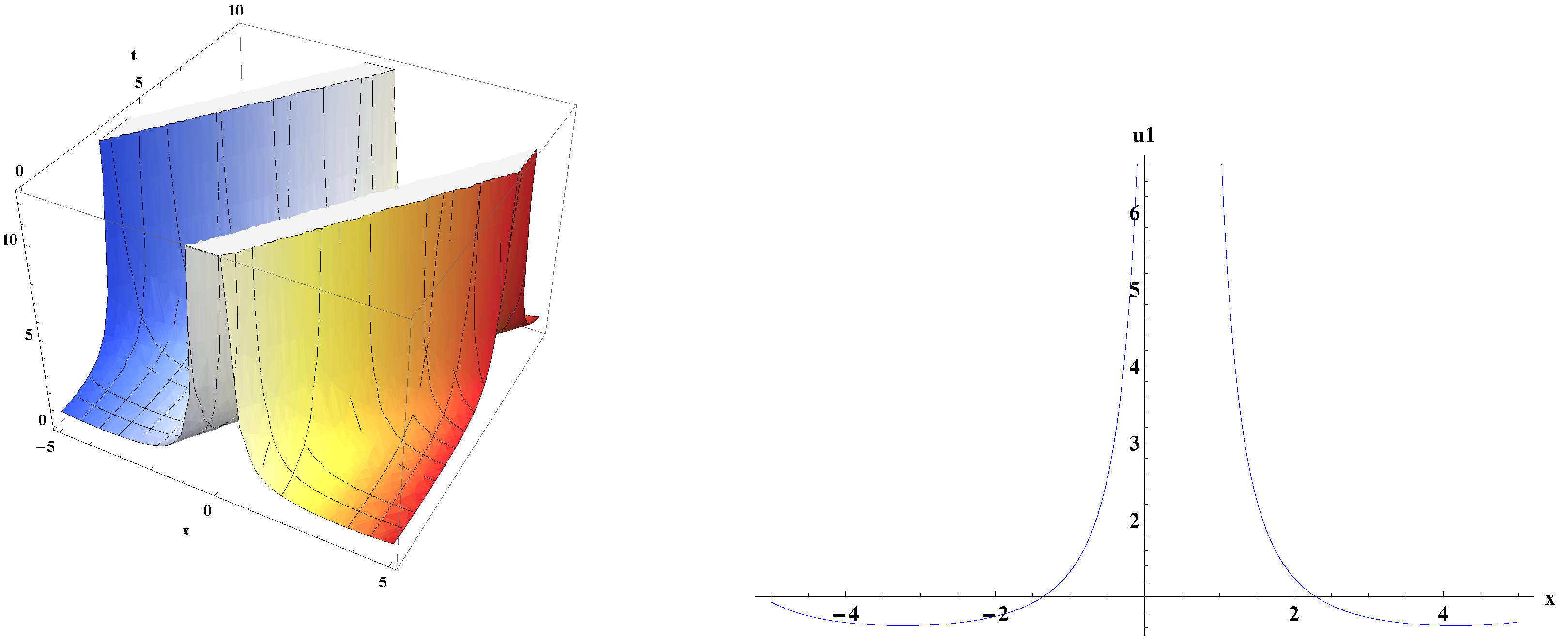
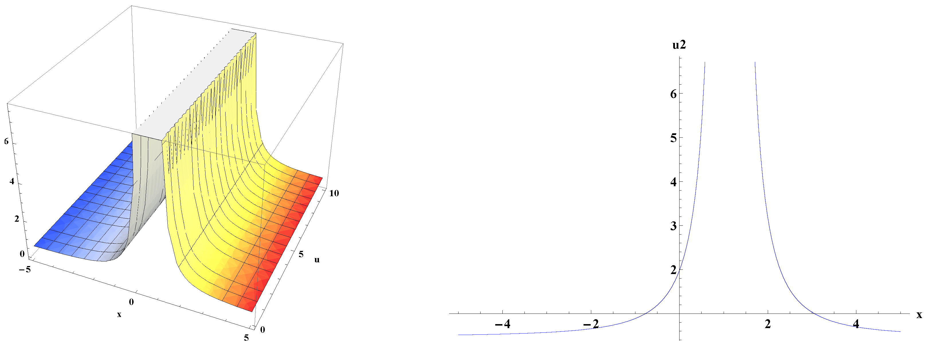
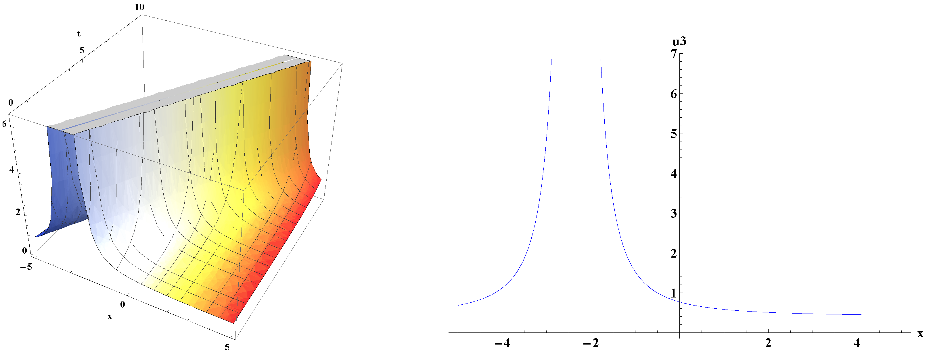
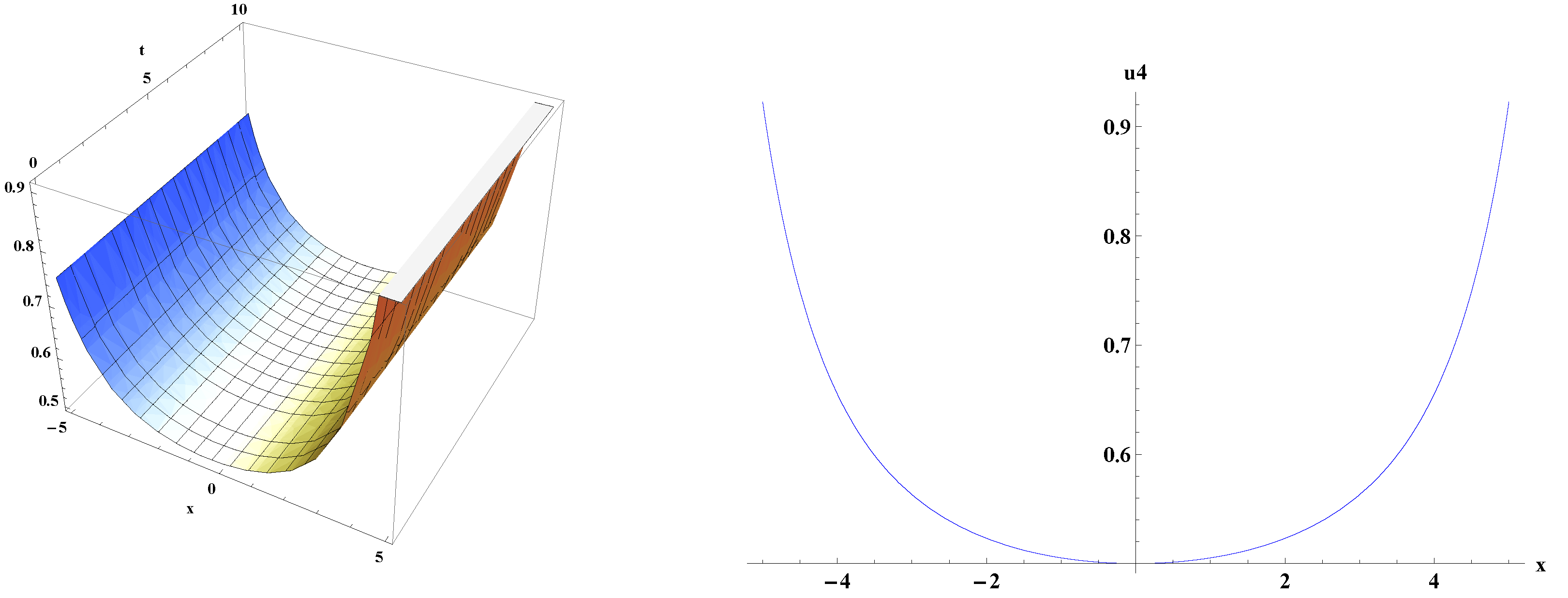
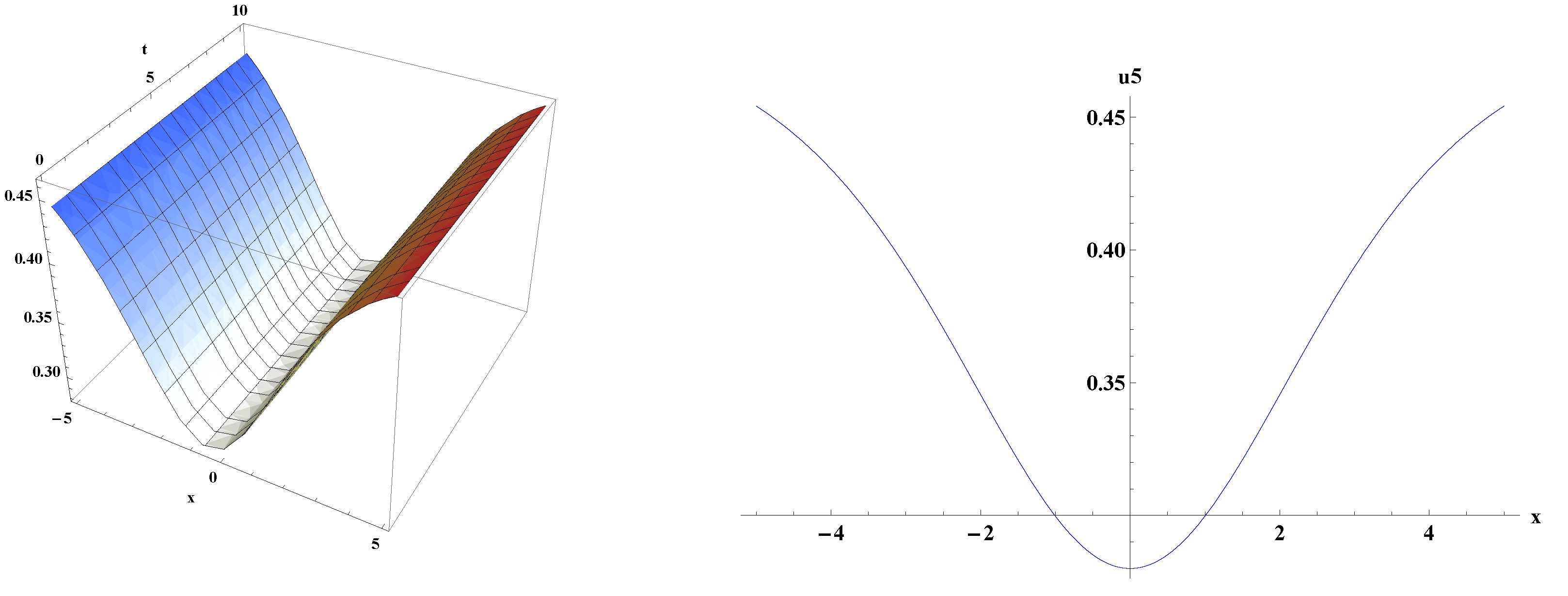
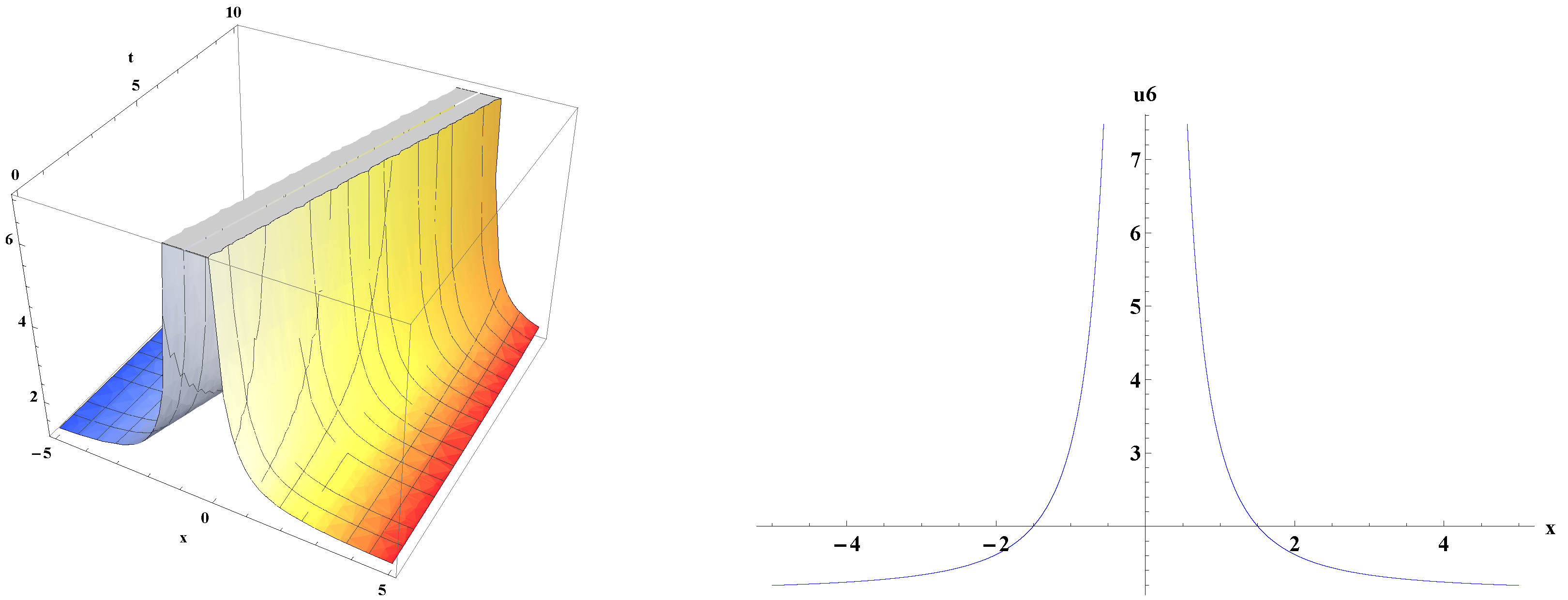
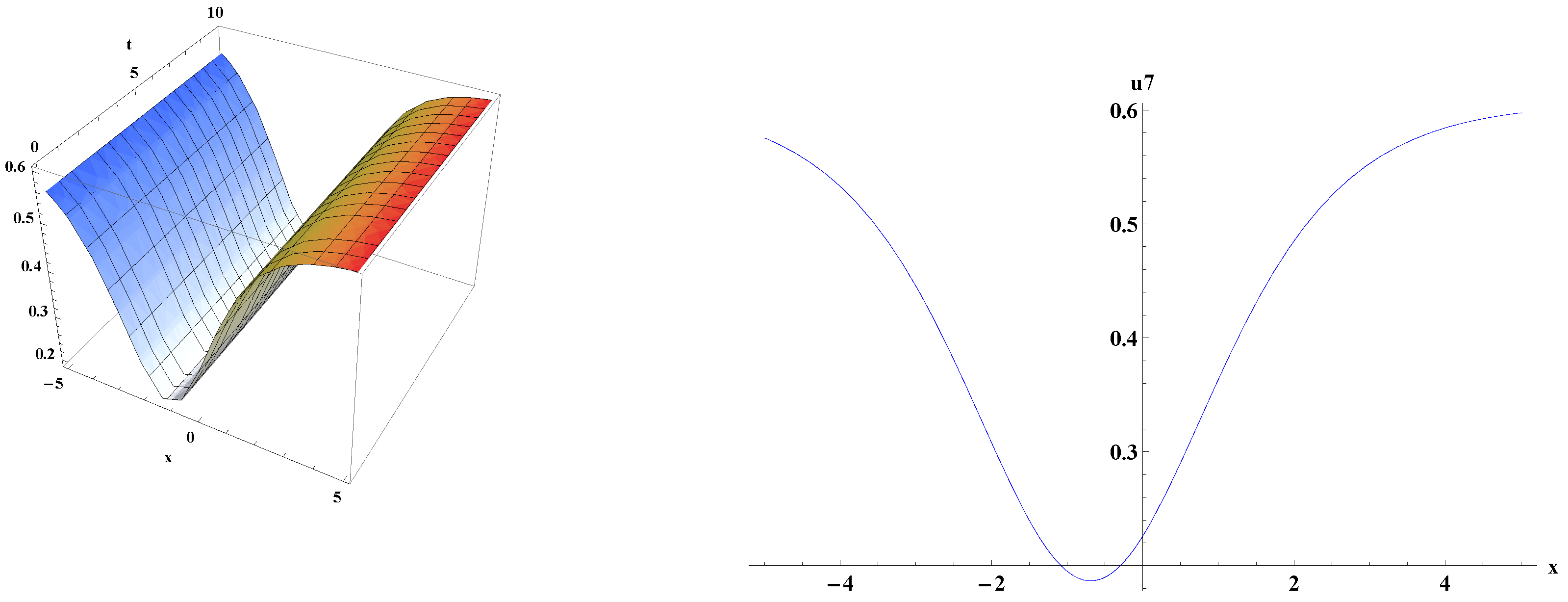
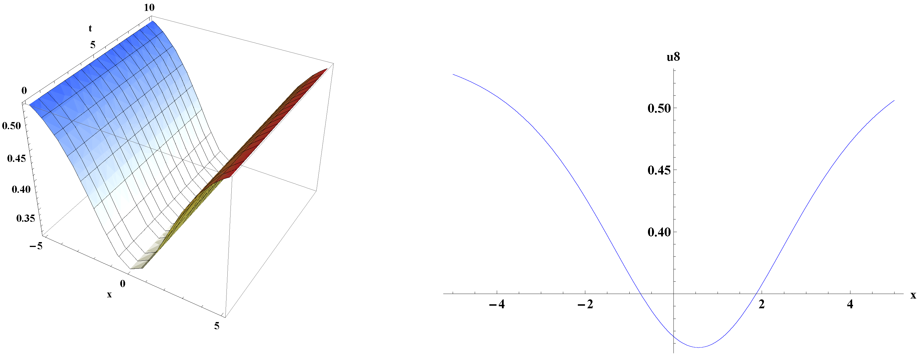
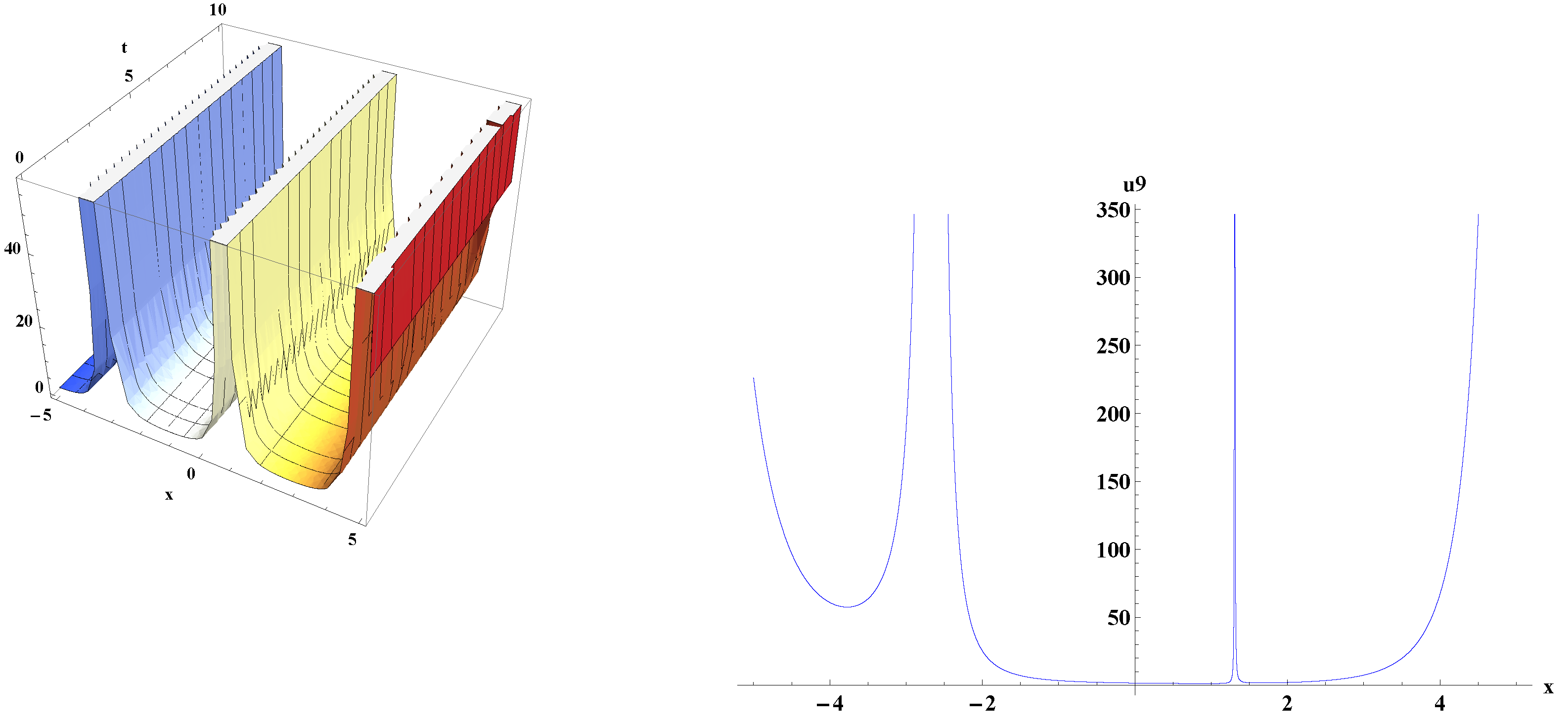
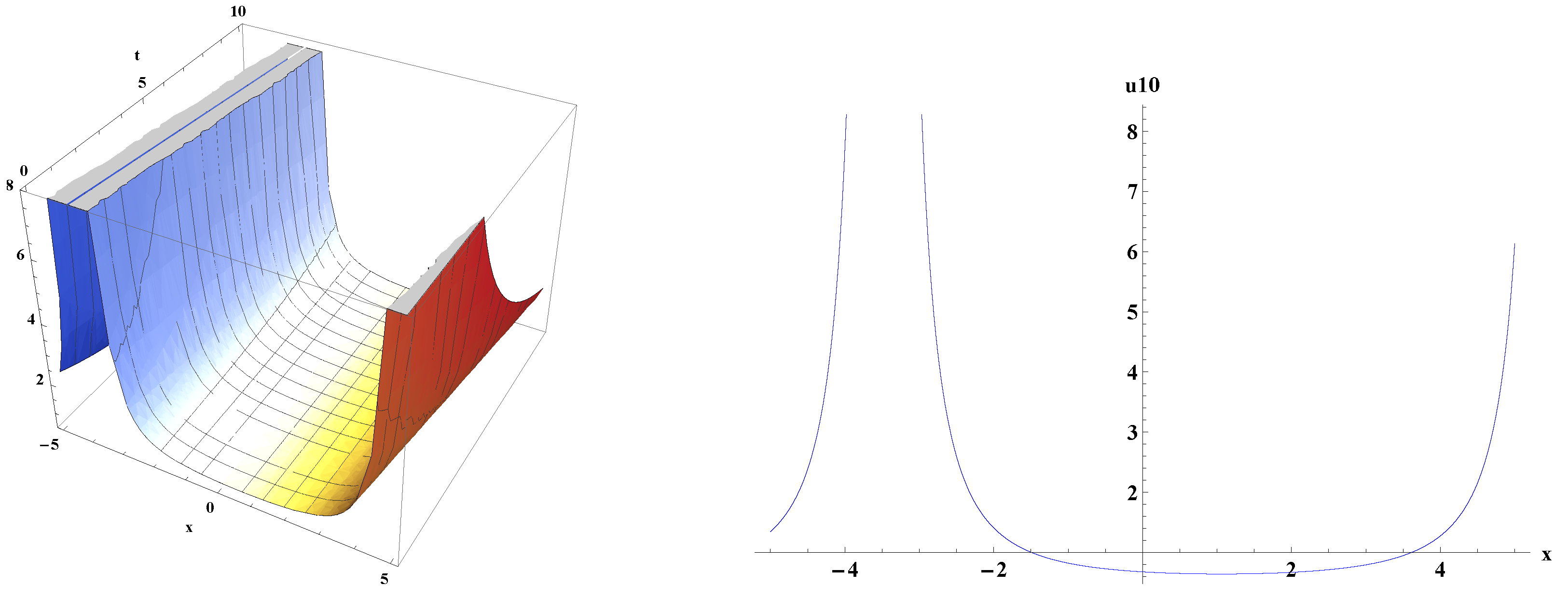
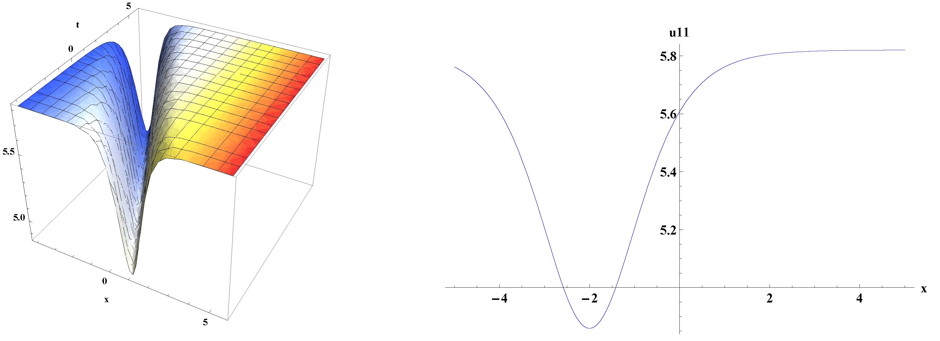
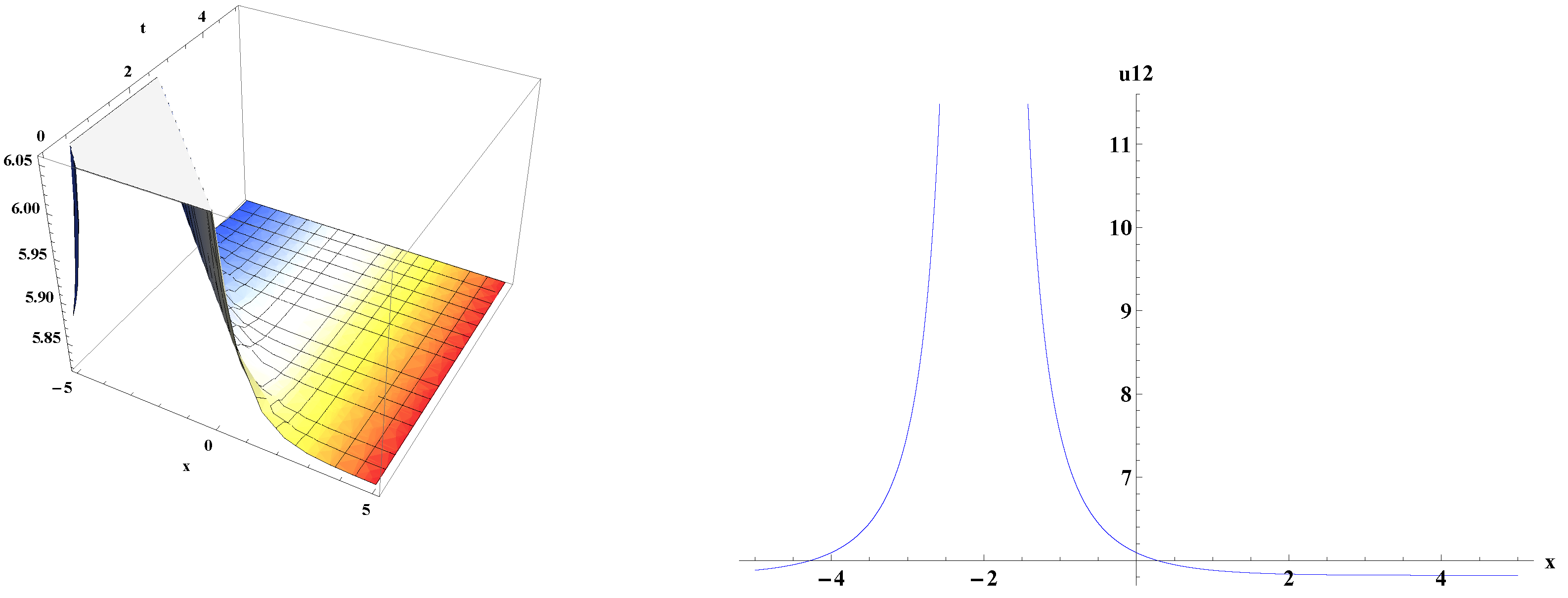
5. Graphical Representations of Traveling Wave Solutions for kp Equation

This section aims to present graphical illustrations of the obtained traveling wave solutions of kp Equation (1). Different types of traveling wave solutions of the desired system can be observed when physical parameters are given by certain values using computer algebra. It is also verified that all of the obtained solutions in this article were valid by inserting them back into the original kp Equation (1). Figure 1, Figure 2 and Figure 3 represent singular wave solutions for kp Equation (1), which were successfully determined in Section 3.1 by using the modified $(g^{\prime }/g^2)$-expansion approach. Solitary waves having a singularity, usually infinite discontinuity, are known as singular soliton solutions. Because this solution involves a spike, it can possibly explain how Rogue waves form. Figure 4, Figure 5 and Figure 6 depict dark and singular wave solutions by using the $\left(g^{\prime }\right)$-expansion approach. The dark solitary wave and singular periodic wave solutions are shown in Figure 7, Figure 8, Figure 9 and Figure 10 by means of the generalized simple $(w/g)$-expansion method (Section 3.3). The obtained traveling wave solutions by akm in Section 4.2 are illustrated in Figure 11 and Figure 12.

6. Conclusions

With the advancement of computer algebra, the investigation of traveling wave solutions for npdes has become a key research area not only in mathematical sciences, but also in many other branches of research such as physics and materials science. In this paper, the extended rational ($w/g$) expansion method is shown to be highly effective and practical for obtaining novel traveling wave solutions for kp Equation (1). To the best of my knowledge, some of these solutions are being obtained for the first time. It has been demonstrated that the extended rational ($g^{\prime }/g^2$)-expansion method is more efficient than the $\left(g^{\prime }\right)$-expansion method, since the former can produce a general form of desired solutions, whilst the latter cannot. Finally, the akm has been successfully described and applied, in Section 4, to obtain new expressions for the traveling wave solutions presented with the support of graphs. It should be emphasized that the presented approaches for obtaining exact traveling wave solutions are both trustworthy, direct, efficient, as well as applicable to a wide range of applications in mathematical physics. Furthermore, these approaches promise a great saving in computation time by using computer algebra such as Mathematica and Maple, which can perform complex and time-consuming algebraic calculations.

References

1. Wazwaz, A.M. Partial Differential Equations and Solitary Waves Theorem; Springer: Berlin, Germany, 2009. [Google Scholar]
2. Grimshaw, R. The solitary wave in water of variable depth. J. Fluid Mech. 1970, 42, 639–656. [Google Scholar] [CrossRef]
3. Baleanu, D.; Machado, A.T.; Luo, A.C.J. Fractional Dynamics and Control; Springer: Berlin/Heidelberg, Germany, 2012; pp. 49–57. [Google Scholar]
4. Boudjehem, B.; Boudjehem, D. Parameter tuning of a fractional-order PI Controller using the ITAE Criteria. In Fractional Dynamics Control; Springer: New York, NY, USA, 2011; pp. 49–57. [Google Scholar]
5. Alotaibi, H. Developing Multiscale Methodologies for Computational Fluid Mechanics. Ph.D. Thesis, University of Adelaide, Adelaide, Australia, 2017. [Google Scholar]
6. Wazwaz, A.M. New Solitary Wave Solutions to the Modified Forms of Degasperis-prcesi and Cassama-Holm Equations. Appl. Math. Comput. 2007, 186, 130–141. [Google Scholar]
7. Gardner, G.S.; Greene, J.M.; Kruskal, M.D.; Mimura, R.M. Method for solving the Korteweg-de-Vries equations. Phys. Rev. Lett. 1967, 19, 1095. [Google Scholar] [CrossRef]
8. Abd-el-Malek, M.B.; Amin, A.M. New exact solutions for solving the initial-value-problem of the KdV-KP equation via the Lie group method. Appl. Math. Comput. 2015, 261, 408–418. [Google Scholar] [CrossRef]
9. Abbasbandy, S. Numerical solutions of nonlinear Klein-Gordon equation by variational iteration method. Int. J. Numer. Meth. Eng. 2007, 70, 876–881. [Google Scholar] [CrossRef]
10. Wazwaz, A.M. A sine-cosine method for handling nonlinear wave equations. Appl. Math. Comput. 2004, 40, 499–508. [Google Scholar]
11. Abdou, M.A. The extended tanh-method and its applications for solving nonlinear physical models. Appl. Math. Comput. 2007, 190, 988–996. [Google Scholar] [CrossRef]
12. Sirendaoreji. New exact traveling wave solutions for the Kawahara and modified Kawahara equations. Chaos Solitons Fractals 2004, 19, 147–150. [Google Scholar] [CrossRef]
13. Akbar, M.A.; Ali, N.H.M. New solitary and periodic solutions of nonlinear evolution equation by exp-function method. World Appl. Sci. J. 2012, 12, 1603–1610. [Google Scholar]
14. He, J.H.; Wu, X.H. Exp-function method for nonlinear wave equations. Chaos Solitons Fractals 2006, 30, 700–708. [Google Scholar] [CrossRef]
15. Khan, K.; Akbar, M.A. Application of (exp(−ϕ(ξ)))-expansion method to find the exact solutions of modified Benjamin-Bona-Mahony equation. World Appl. Sci. J. 2013, 10, 1373–1377. [Google Scholar]
16. Wu, L.; Chen, S.; Pang, C. Traveling wave solution for Generalized Drinfeld-Sokolov equations. Appl. Math. Model. 2009, 33, 4126–4130. [Google Scholar] [CrossRef]
17. Zhang, F.; Qi, J.M.; Yuan, W.J. Further results about traveling wave exact solutions of the Drinfeld-Sokolov equations. J. Appl. Math. 2013, 2013, 523732. [Google Scholar] [CrossRef]
18. Kaplan, M.; Bekir, A.; Akbulut, A. A generalized Kudryashov method to some nonlinear evolution equations in mathematical physics. Nonlinear Dyn. 2016, 85, 2843–2850. [Google Scholar] [CrossRef]
19. Zayed, E.M.; Shohib, R.M.; Alngar, M.E. New extended generalized Kudryashov method for solving three nonlinear partial differential equations. Nonlinear Anal. Model. Control 2020, 25, 598–617. [Google Scholar] [CrossRef]
20. Alotaibi, H. Traveling Wave Solutions to the Nonlinear Evolution Equation Using Expansion Method and Addendum to Kudryashov’s Method. Symmetry 2021, 13, 2126. [Google Scholar] [CrossRef]
21. Gepreel, K.A. Exact Soliton Solutions for Nonlinear Perturbed Schrödinger Equations with Nonlinear Optical Media. Appl. Sci. 2020, 10, 8929. [Google Scholar] [CrossRef]
22. Zhong, B.; Jiang, J.; Feng, Y. New exact solutions of fractional Boussinesq-like equations. Commun. Optim. Theory 2020, 1–17. [Google Scholar] [CrossRef]
23. Zayed, E.M.E.; Gepreel, K.A.; El-Horbaty, M.; Biswas, A.; Yıldırım, Y.; Alshehri, H.M. Highly Dispersive Optical Solitons with Complex Ginzburg-Landau Equation Having Six Nonlinear Forms. Mathematics 2021, 9, 3270. [Google Scholar] [CrossRef]
24. Laouini, G.; Amin, A.M.; Moustafa, M. Lie Group Method for Solving the Negative-Order Kadomtsev–Petviashvili Equation (nKP). Symmetry 2021, 13, 224. [Google Scholar] [CrossRef]
25. Johnson, R.S. Water waves and Korteweg-de Vries equations. J. Fluid Mech 1980, 97, 701–719. [Google Scholar] [CrossRef]
26. Demiray, H. Weakly nonlinear waves in water of variable depth: Variable-coefficient Korteweg-de Vries equation. Comput. Math. Appl. 2010, 60, 1747–1755. [Google Scholar] [CrossRef]
27. Khan, K.; Akbar, M.A. Exact traveling wave solutions of Kadomtsev–Petviashvili equation. J. Egypt. Math. Soc. 2015, 23, 278–281. [Google Scholar] [CrossRef] [Green Version]
28. Chen, Y.; Yan, Z.; Zhang, H. New explicit solitary wave solutions for (2+1)-dimensional Boussinesq equation and (3+1)-dimensional KP equation. Phys. Lett. 2003, 307, 107–113. [Google Scholar] [CrossRef]
29. Roshid, M.M.; Roshid, H.O. Exact and explicit traveling wave solutions to two nonlinear evolution equations which describe incompressible viscoelastic Kelvin-Voigt fluid. Heliyon 2018, 4, e00756. [Google Scholar] [CrossRef] [Green Version]
30. El-Sayed, S.M.; Kaya, D. The decomposition method for solving (2+1)-dimensional Boussinesq equation and (3+1)-dimensional KP equation. Appl. Math. Comput. 2004, 157, 523–534. [Google Scholar] [CrossRef]
31. Wazwaz, A.M. Multiple-soliton solutions for the KP equation by Hirota’s bilinear method and by the tanh-coth method. Appl. Math. Comput. 2007, 190, 633–640. [Google Scholar] [CrossRef]
32. Moslem, W.M.; Abdelsalam, U.M.; Sabry, R.; El-Shamy, E.F.; El-Labany, S.K. Three-dimensional cylindrical Kadomtsev–Petviashvili equation in a dusty electronegative plasma. J. Plasma Phys. 2010, 76, 453–466. [Google Scholar] [CrossRef]
33. Li, W.-A.; Chen, H.; Zhang, G.-C. The (w/g)-expansion method and its application to Vakhnenko equation. Chin. Phys. B 2009, 18, 400. [Google Scholar]
34. Wang, M.; Li, X.; Zhang, J. The (G′/G)-expansion method and traveling wave solutions of nonlinear evolution equations in mathematical physics. Phys. Lett. 2008, 372, 417–423. [Google Scholar] [CrossRef]
35. Attia, M.T.; Elhanbaly, A.; Abdou, M.A. New exact solutions for isothermal magne to static atmospheres equations. Walailak J. Sci. Technol. 2014, 12, 961–973. [Google Scholar]
36. Wang, M.; Li, X.Z. Extended F-expansion method and periodic wave solutions for the generalized Zakharov equations. Phys. Lett. A 2005, 343, 48–54. [Google Scholar] [CrossRef]
37. Gepreel, K.A. Exact solutions for nonlinear integral member of Kadomtsev–Petviashvili hierarchy differential equations using the modified (w/g)-expansion method. Comput. Math. Appl. 2016, 72, 2072–2083. [Google Scholar] [CrossRef]
38. Abdusalam, H.A. On an improved complex tanh-function method. Int. J. Nonlinear Sci. Numer. Simul. 2005, 6, 99–106. [Google Scholar] [CrossRef]
39. Zayed, E.M.; Zedan, H.A.; Gepreel, K.A. Group analysis and modified extended Tanh- function to find the invariant solutions and soliton solutions for nonlinear Euler equations. Int. J. Nonlinear Sci. Numer. Simul. 2004, 5, 221–234. [Google Scholar] [CrossRef]
40. Kudryashov, N.A. Method for finding highly dispersive optical solitons of nonlinear differential equations. Optik 2020, 206, 163550. [Google Scholar] [CrossRef]
41. Zayed, E.M.E.; Alngar, M.E.M.; Biswas, A.; Kara, A.H.; Ekici, M.; Alzahrani, A.K.; Belic, M.R. Cubicquartic optical solitons and conservation laws with Kudryashov’s sextic power-law of refractive index. Optik 2021, 227, 166059. [Google Scholar] [CrossRef]
Figure 1. Singular periodic solution (13) (left) and its projections at t = 0 (right), when a = 0.6 , c = 0.3 , δ = 1 ,   k = 0.7 ,   A 1 = 0.5 ,   A 2 = 0.1 , and y = 0.5 .
Crystals 12 00159 g001
Figure 2. Singular wave solution (14) (left) and its projections at t = 0 (right), when a = 0.2 , c = 0.3 , δ = 1 ,   k = 0.3 ,   A 1 = 0.4 ,   A 2 = 0.7 , and y = 0.5 .
Crystals 12 00159 g002
Figure 3. Singular wave solution (15) (left) and its projections at t = 0 (right), when a = 0 , c = 0.4 , δ = 1 ,   k = 0.6 ,   A 1 = 0.3 ,   A 2 = 0.7 , and y = 0.5 .
Crystals 12 00159 g003
Figure 4. Dark wave solution (18) (left) and its projections at t = 0 (right), when a = 0.3 ,   c = 0.2 , δ = 1 , k = 0.4 ,   b = 0.2 , and y = 0.5 .
Crystals 12 00159 g004
Figure 5. Dark wave solution (19) (left) and its projections at t = 0 (right), when a = 0.4 , c = 0.2 , δ = 1 ,   k = 0.5 , b = 0.3 , and y = 0.5 .
Crystals 12 00159 g005
Figure 6. Singular solitary wave solution (20) (left) and its projections at t = 0 (right), when a = 1 , c = 1 ,   δ = 1 ,   k = 0.3 ,   b = 2 , and y = 0.5 .
Crystals 12 00159 g006
Figure 7. Dark solitary wave solution (24) (left) and its projections at t = 0 (right), when A 1 = 0.1 , A 2 = 0.5 ,   μ = 0.7 ,   λ = 0.3 ,   k = 0.2 ,   δ = 1 , and y = 0.5 .
Crystals 12 00159 g007
Figure 8. Dark solitary wave solution (25) (left) and its projections at t = 0 (right), when A 1 = 0.2 , A 2 = 0.9 ,   μ = 0.3 ,   λ = 0.4 ,   k = 0.2 ,   δ = 1 , and y = 0.5 .
Crystals 12 00159 g008
Figure 9. Singular periodic wave solution (26) (left) and its projections at t = 0 (right), when A 1 = 0.4 , A 2 = 0.6 ,   μ = 0.7 ,   λ = 0.9 ,   k = 0.2 ,   δ = 1 , and y = 0.5 .
Crystals 12 00159 g009
Figure 10. Singular periodic wave solution (27) (left) and its projections at t = 0 (right), when A 1 = 0.4 , A 2 = 0.9 ,   μ = 0.4 ,   λ = 0.3 ,   k = 0.1 ,   δ = 1 , and y = 0.5 .
Crystals 12 00159 g010
Figure 11. Dark wave solution (36) (left) and its projection at t = 0 (right), when K = 2 ,   k = 2 ,   δ = 3 , and y = 2 .
Crystals 12 00159 g011
Figure 12. Singular wave solution (37) (left) and its projection at t = 0 (right), when K = 2 ,   k = 2 , δ = 3 , and y = 2 .
Crystals 12 00159 g012
Publisher’s Note: MDPI stays neutral with regard to jurisdictional claims in published maps and institutional affiliations.