A Multi-Objective Identification of DEM Microparameters for Brittle Materials

1. Introduction

The discrete element method (DEM) [1] has been widely used by researchers and engineers to research the mechanical characteristics of brittle materials, such as granular material and rock [2,3,4,5,6]. Considering the material failure properties and various kinds of discontinuities, DEM can simulate and analyze the fracture mode and large deformations [7,8,9]. When constructing the DEM model, the contact models are adopted to describe the mechanical behaviors in real materials. Generally, the contact model contains a number of microparameters, which reflect the behavior of the material at the micro-level. It is essential to identify these input parameters to perform DEM computations. In other words, the success of DEM calculation depends on the accuracy of these microparameters.

One crucial challenge of DEM is how to accurately determine the microparameters. Some parameters can be identified directly from experimental tests, while it is difficult to determine others as the measured results from the experiment are macro-responses. Traditionally, a “trial and error” method is utilized to identify these parameters through an iterative way of varying the value of parameters until the DEM computational results match the experimental results [10,11]. Although this method is simple, it has several obvious disadvantages. It may be time-consuming to run a number of DEM calculations to obtain the desired results. Furthermore, it may be full of randomness and experience is needed for parameter identification with this approach. Additionally, as the number of parameters increases, the accuracy of the identified results and the efficiency may be much lower. In order to handle these obstacles, it is necessary to seek an appropriate method to determine the DEM parameters.

With the great progress in research on inverse problem and intelligent algorithm, the method based on inverse technique gets more and more suitable to identify the model parameters [12,13,14]. In this method, the research in parameter identification is transformed to an optimization research and then the parameters are identified by using an optimization algorithm to minimize the objective function, which usually describes the deviation between the computational results and experimental data. Many researchers have presented the inverse approach to determine the DEM microparameters [15,16,17,18]. Yoon [19] used the design of experiment (DOE) method and optimization algorithm to determine some microparameters of the DEM model for rock with uniaxial compressive tests. Tawadrous et al. [20] utilized an artificial neural networks (ANN) method to determine DEM microparameters for a uniaxial compressive model for rock material. Kazerani [21] combined the central composite design (CCD) method with statistical analysis to estimate the DEM input parameters of Augig granite under a compressive test and tensile test, respectively. Do et al. [22] adopted a genetic and DIRECT optimization algorithm to obtain the microparameters of the DEM model for quartz sand. Simone et al. [23] adopted the CCD method and genetic algorithm to identify the DEM microparameters under uniaxial compression. These identified results indicated that the DEM input parameters were determined quickly and effectively by these methods. In these studies, the microparameters were usually determined with one kind of experimental condition, in which single-objective optimization was used. However, when only considering a single experiment during parameter identification, it may cause these parameters to be valid for one case (e.g., compression test) but fail for another (e.g., tensile test); especially for rock-like materials, the mechanical characteristics are very complex under different loadings. Hence, it is of great significance to identify the input parameters of DEM for rock by considering different experimental conditions.

In recent years, many multi-objective optimization algorithms have been presented to deal with multi-objective optimization problems with good performances [24,25,26]. It can obtain the optimal solutions under different conditions and has been applied to parameter identification. Milani et al. [27] proposed a weighted multi-objective identification technique to determine the key parameters of the Johnson–Cook constitutive model for metal materials with split Hopkinson pressure bar tests and a quasi-static test. Papon et al. [28] utilized the multi-objective genetic algorithm to identify the parameters of the Mohr–Coulomb model and elaso-plastic model for soil. Consequently, in order to overcome the abovementioned problem, a multi-objective identification method is developed to identify the DEM microparameters. In this method, the identification problem for the DEM input parameters is converted into a multi-objective optimization research and the micro-multi-objective genetic algorithm (µMOGA) is utilized to solve this problem. Firstly, a set of experiments are carried out to provide input and output data, and then the corresponding DEM models are constructed. Secondly, sensitivity analysis is done to investigate the influence of the input parameters on the computational responses and then the inversed parameters are obtained. Moreover, the approximation model technique is employed for replacing the actual DEM computations to improve computational efficiency. Finally, the inversed microparameters are identified by µMOGA and the validations are performed.

The structure of this paper is as follows: Section 2 presents an overview of the multi-objective identification technique. Section 3 provides detailed solution steps. Section 4 gives the results and discussion of the solution, and Section 5 provides the conclusion.

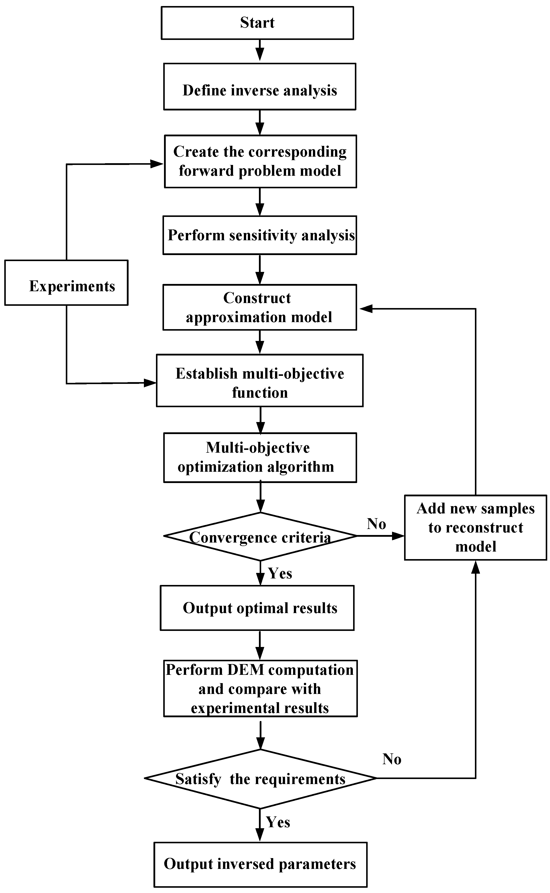
2. Multi-Objective Identification Technique

This study aims to identify the DEM microparameters with different material experiments by a multi-objective identification technique. The flowchart of this identification technique is showed in Figure 1. First of all, it is essential to investigate the physical and mechanical characteristics of the material, then different experiments are carried out to obtain the corresponding responses, which are the input values and validation data for parameter identification. Secondly, on the basis of these experiments, the corresponding DEM numerical model is built and an appropriate contact model is selected to describe the material properties, which is considered as the establishment of the forward problem. In order to reduce ill-posed elements and ensure high sensitivity between responses and the inversed parameters, the microparameters sensitivity analysis of the contact model is performed and then the inversed variables are obtained. Furthermore, the approximation model technique is adopted to replace the DEM calculations for improving the computational efficiency. Based on the computational results and experimental measurement, a multi-objective function is built and a multi-objective optimization problem is constructed. Moreover, µMOGA is employed as an inverse operator to solve this optimization problem. In this study, the multi-objective optimization problem aims to minimize the relative deviation between the DEM computational results and the experimental data under different experimental conditions, which can be expressed as follows:

$$Min\left\{\begin{array}{ccc}{f}_1\left(\mathit{x}\right),& \cdots ,& f_m\left(\mathit{x}\right)\end{array}\right\}$$

(1)

$$f_i\left(\mathit{x}\right)={\displaystyle {\displaystyle \sum }_{j=1}^n}\frac{\left|y_j^c-y_j^{ex}\right|}{y_j^{ex}} i=1,\cdots ,m$$

(2)

where $f_i$ stands for a single-objective function, which describes the relative deviation between the DEM computational results and experimental data under one experimental test. $\mathit{x}$ is the vector of the inversed input parameters and $m$ is the total number of experimental cases. $y_j^c$ is the DEM computational responses, $y_j^{ex}$ is the experimental measured responses, and $n$ is the number of response variables.

While solving this problem, the convergence criteria should be set and the results could be obtained by meeting the convergence criteria. If they are not met, new samples should be added to reconstruct the approximation model and repeat the previous steps. Then, the inversed parameters could be initially determined by solving the inverse problem. Finally, verification and validation should be performed to verify the effectiveness and reliability. Given this, a set of DEM computations with the inversed results for different conditions are carried out and the comparisons between the DEM computed results and the experimental measurements are conducted. If the requirements are satisfied, the values of the inversed parameters are outputted. Otherwise, the approximation model should be reconstructed by adding new samples and then repeating the previous steps until the optimal results are obtained. Consequently, the DEM microparameters can be identified by the presented technique, which mainly consists of material experimental tests, DEM computation, a sensitivity analysis, and an approximation model and multi-objective optimization algorithm—the details of each part will be presented in later sections.

3. DEM Microparameters Identification for Granite

In order to demonstrate the performance of the developed multi-objective identification technique, the identification of DEM microparamters for granite material is performed. In this study, three different experimental tests for granite (uniaxial compression, Brazilian splitting, and the three-point bending test) are conducted for providing input and verification and validation data. The uniaxial compression test and Brazilian splitting test are utilized to determine and verify the DEM microparameters by comparing macro-responses on the Poisson’s ratio, Young’s modulus, and the maximum uniaxial tensile strength and maximum uniaxial compressive strength obtained from the DEM calculation and experimental measurements. Then, the three-point bending test is used to validate the inversed parameters through fracture toughness obtained from DEM computation and experimentation.

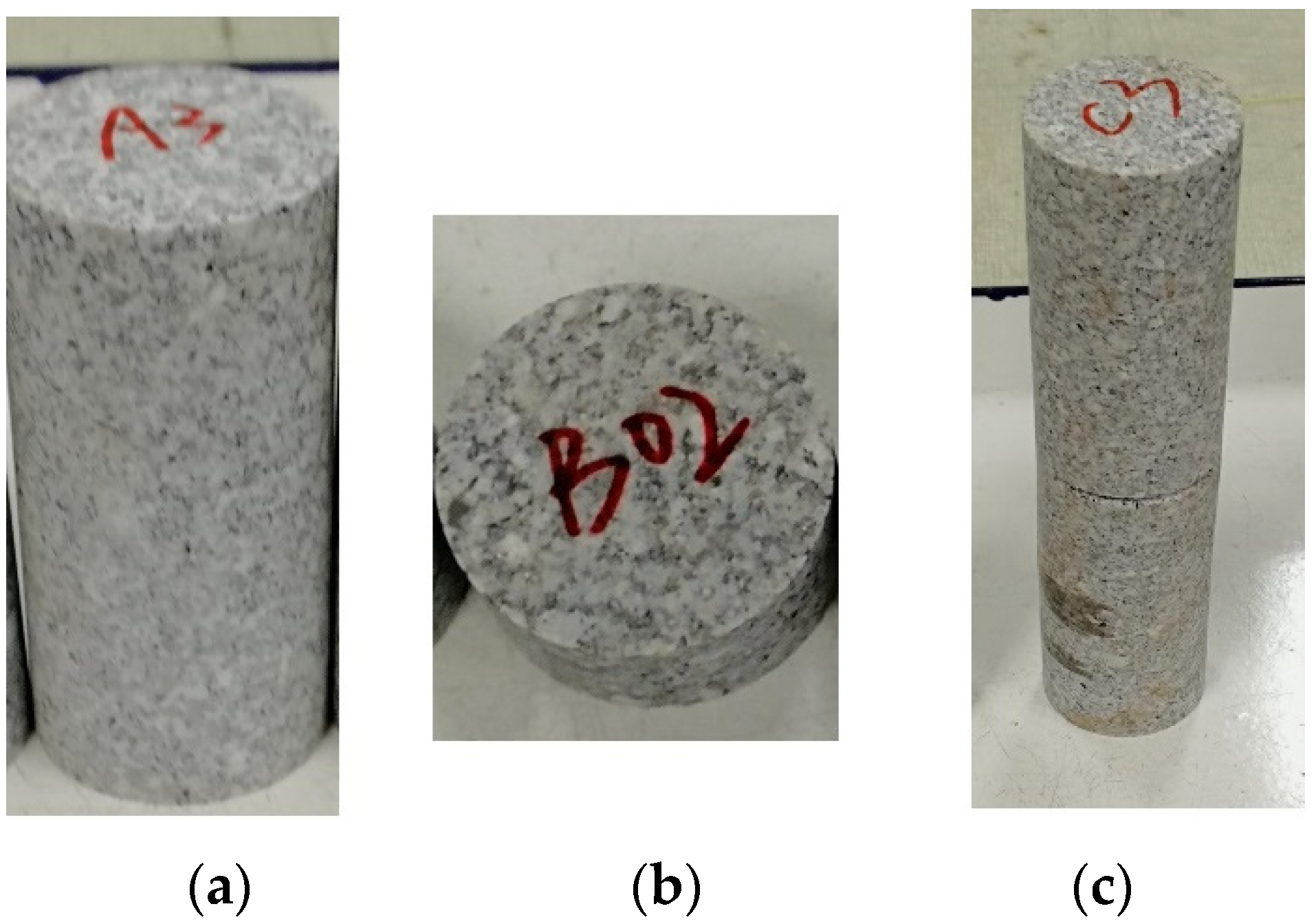
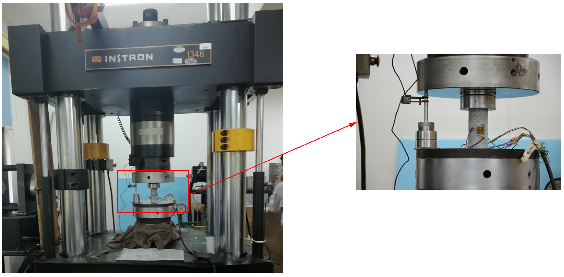
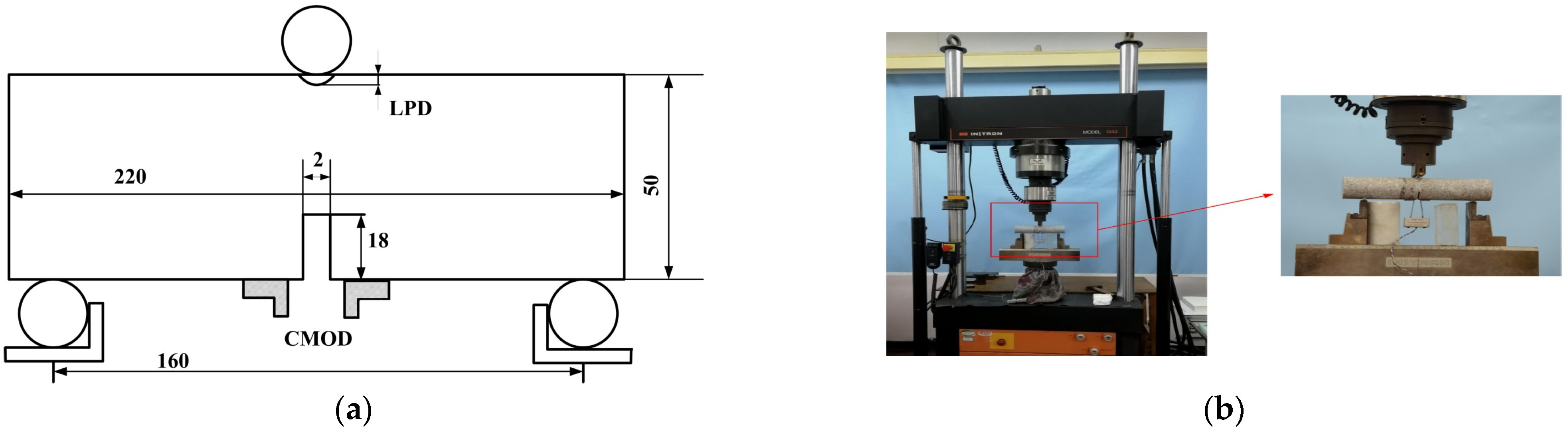
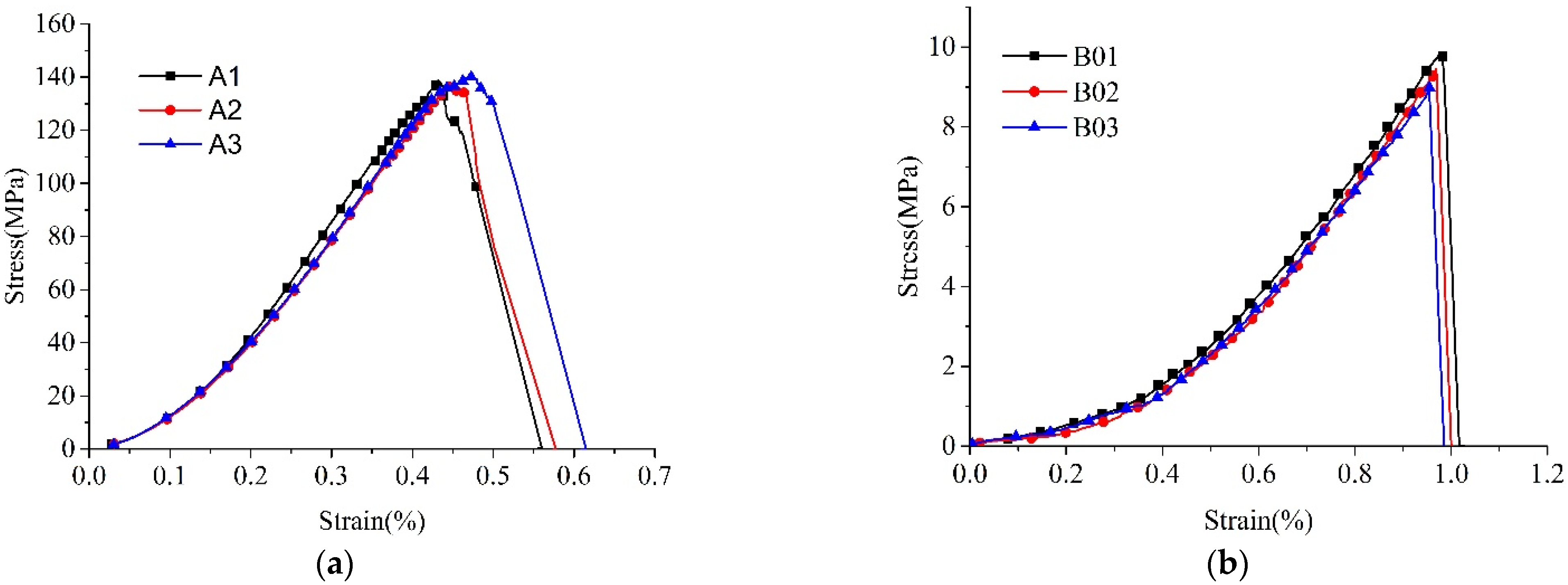
3.1. Experimental Measurement

As shown in Figure 2, granite specimens with three different sizes were made for the tests. The cylindrical specimens with $\phi 50\hspace{0.17em}\mathrm{mm}\times 100\hspace{0.17em}\mathrm{mm}$ and $\phi 50\hspace{0.17em}\mathrm{mm}\times 25\hspace{0.17em}\mathrm{mm}$ were used for the Brazilian splitting and uniaxial compression tests, respectively. The cylindrical specimens with a single-edge notch (the dimensions of the specimen are $\phi 50\hspace{0.17em}\mathrm{mm}\times 200\hspace{0.17em}\mathrm{mm}$ and the dimensions of the notch are 18 mm in length and 2 mm in width) were used for the three-point bending tests. In the tests, A, B, and C denote the uniaxial compression, Brazilian splitting, and three-point bending test, respectively. The Instron 1346 hydraulic servo-controlled machine was used to conduct the uniaxial compression tests, as shown in Figure 3. Additionally, the Instron 1342 hydraulic servo-controlled machine was used to conduct the Brazilian splitting and three-point bending tests, as shown in Figure 4 and Figure 5. In the three-point bending test, the crack opening displacement (COD) transducer is used to measure the crack opening displacement occurring within the gauge on the surface. Furthermore, the measuring accuracy of the transducers is 0.001 mm.

The measured results from the three different kinds of experiments were given in Figure 6 and Figure 7. From these figures, it can be seen that the experimental measured data have a good reproducibility and the results have a fine reliability. Then, through the processing of the experimental data, several macro-responses of granite can be obtained and the value of the variable is the average of the measured results. Hence, the basic mechanical property parameters of granite were listed in

Table 1. The basic mechanical properties of Granite.

$\mathit{\rho }$ (kg/m3)	$\mathit{E}$ (GPa)	$\mathit{\nu }$	${\mathit{\sigma }}_{\mathit{c}}$ (MPa)	${\mathit{\sigma }}_{\mathit{t}}$ (MPa)	${\mathit{K}}_{\mathit{I}\mathit{C}}.$ (MPa·m1/2)
2622	41.5	0.23	138.8	9.5	1.057

, which include Poisson’s ratio $\nu$, uniaxial compression strength ${\sigma }_c$, density $\rho$, Young’s modulus $E$, fracture toughness $K_{IC}$, and uniaxial tensile strength ${\sigma }_t$.

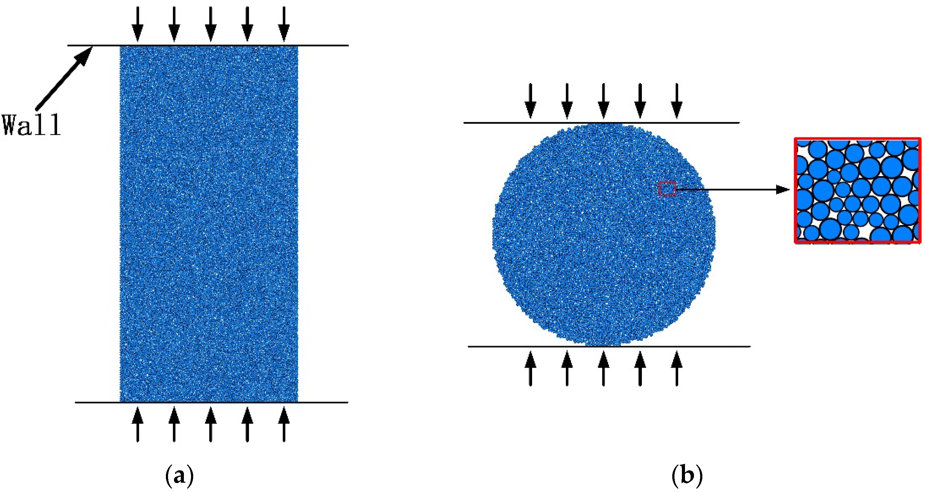
3.2. DEM Model and Its Microparameters

In this study, as the uniaxial compression test and Brazilian splitting test were applied to determine the DEM model parameters, the corresponding DEM numerical model was built, as shown in Figure 8. For the purpose of improving the computational efficiency, the 2-dimension discrete element model was built. The geometric dimensions and the boundary and loading conditions of the DEM models were the same as those of the actual experiments. Additionally, the number of particles is the key issue for the DEM model. Generally, the more the number of particles there are, the higher the model accuracy is. In this work, the number of particles for the DEM models under uniaxial compression and Brazilian splitting were 12,952 and 6100, respectively. Furthermore, the minimum radius for the particle and the maximum-to-minimum radius ratio for the DEM models were 0.25 mm and 1.66, respectively.

The bond particle model (BPM) is one of the most commonly used contact models in DEM, which represents the various mechanical properties of rock-like materials, including elasticity and fracturing [29]. In BPM, there are two forms, including parallel bonds and contact bonds. The parallel bond is not only able to transmit the tension and shear force between the particles, but also to transmit the moment and torque between the particles. In this study, the parallel bond of the BPM was adopted to describe the mechanical behaviors of granite.

As described in reference [29], there were eight microparameters in the BPM model, containing the normal-to-shear stiffness ratios of the ball $K_n/K_s$, the bond effective modulus $\overline{E_c}$, the ball effective modulus $E_c$, the parallel bond radius multiplier $\mathsf{\lambda }$, the shear strength of the parallel bond ${\overline{\tau }}_{\mathrm{c}}$, the particles friction coefficient $\mathsf{\mu }$, the tensile strength of the parallel bond ${\overline{\sigma }}_{\mathrm{c}}$, and the normal-to-shear stiffness ratios of the parallel bond $\overline{K_n}/\overline{K_s}$. Some researchers [29,30] have investigated these parameters and pointed out that the stiffness ratio of the ball can be equal to the stiffness ratio of the parallel bond; the ball effective modulus can be equal to the bond effective modulus; and the radius multiplier of the parallel bond $\mathsf{\lambda }$ is set to 1 to produce a material with cement that completely fills the throat between the cemented particles. Consequently, there were five unknown microparameters ($E_c$, $K_n/K_s$, ${\overline{\sigma }}_c$, ${\overline{\tau }}_{\mathrm{c}},$and $\mathsf{\mu }$), which were very difficult to be directly determined from their values from the experiments.

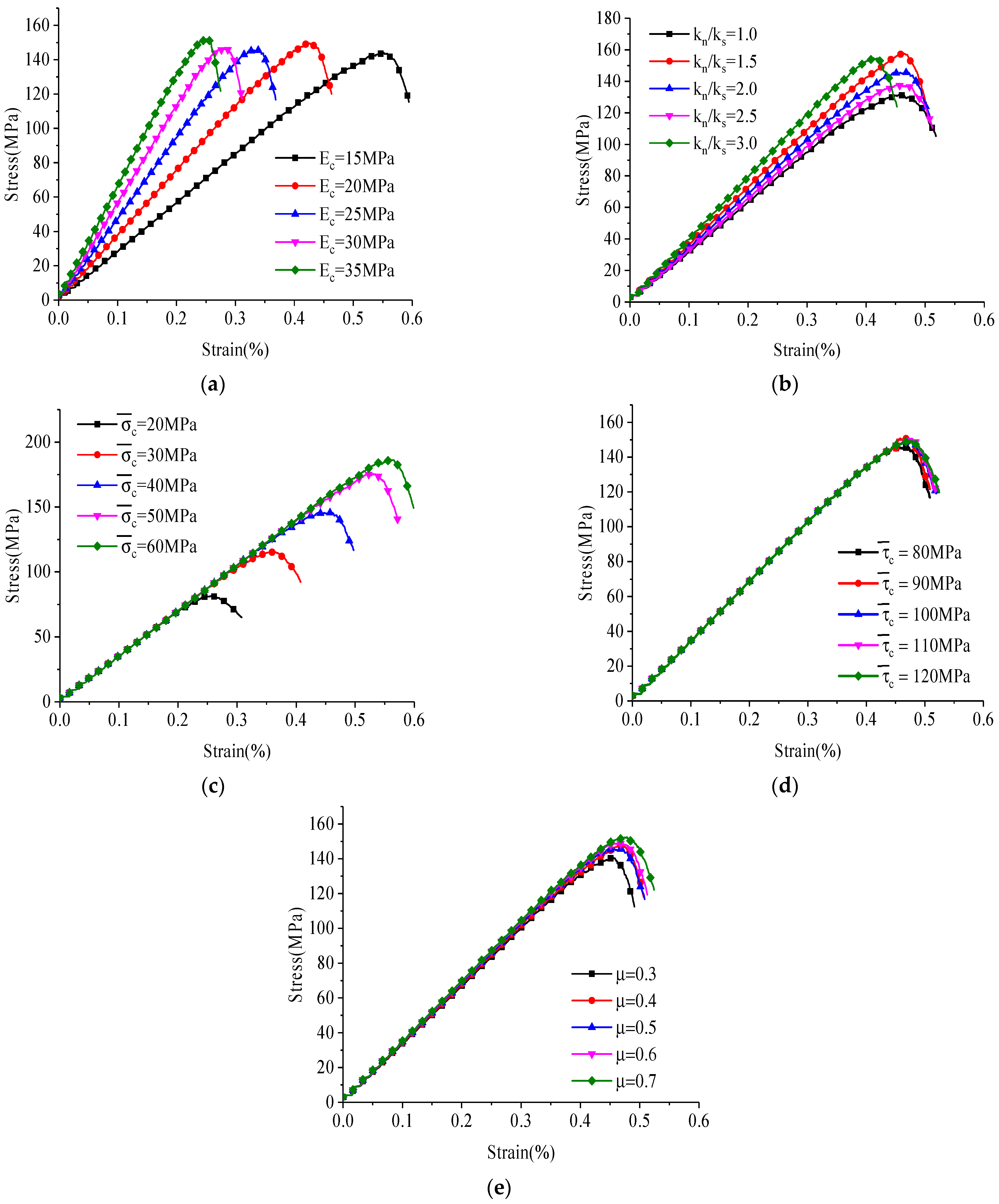
3.3. Parameter Sensitivity Analysis

During parameter identification by the inverse method, the inversed parameters should have a high sensitivity to the output responses for reducing any ill-posed elements. Given this, a sensitivity analysis of the unknown parameters combined with numerical calculations was carried out to estimate the relationship between the inversed parameters and responses.

In this work, a series of DEM computations under uniaxial compression and Brazilian splitting conditions were performed for the sensitivity analysis. Firstly, the initial values for the unknown parameters should be set ($E_c$ is 25 GPa, $K_n/K_s$ is 2, ${\overline{\sigma }}_c$ is 40 MPa, ${\overline{\tau }}_c$ is 100 MPa, and $\mathsf{\mu }$ is 0.5). Then, four values for each parameter were given, as listed in

Table 2. Four values of each parameter for sensitivity analysis.

No.	${\mathit{E}}_{\mathit{c}} (\mathbf{GPa})$	${\mathit{k}}_{\mathit{n}}/{\mathit{k}}_{\mathit{s}}$	${\overline{\mathit{\sigma }}}_{\mathit{c}} (\mathbf{MPa})$	${\overline{\mathit{\tau }}}_{\mathit{c}} (\mathbf{MPa})$	μ
1	15	1	20	80	0.3
2	20	1.5	30	90	0.4
3	30	2.5	50	110	0.6
4	35	3	60	120	0.7

. For the sensitivity analysis of one parameter, the values of this parameter were varied and the other four parameters’ values were still set to the initial values. Given this, the DEM calculation could be performed five times for one parameter’s sensitivity analysis under one experimental condition.

The results of the parameters’ sensitivity analysis under the uniaxial compressive case and Brazilian splitting case were shown in Figure 9 and Figure 10. It can be seen that the variation trend of macro-computational responses was similar to the change of each parameter’s value both under the uniaxial compressive and Brazilian splitting case. It is also found that the responses varied greatly with parameters $K_n/K_s$, $E_c$, and ${\overline{\sigma }}_c$ varying dependently, which meant that $K_n/K_s$, $E_c$, and ${\overline{\sigma }}_c$ were highly sensitive to the responses. However, the changes in the values of parameters ${\overline{\tau }}_c$and $\mathsf{\mu }$ had little effect on the responses, which indicated that ${\overline{\tau }}_c$and $\mathsf{\mu }$ were lowly sensitive to the responses. Based on these results from the sensitivity analysis, the three unknown parameters $K_n/K_s$, $E_c$, and ${\overline{\sigma }}_c$ are defined as inversed parameters. Furthermore, based on the experimental measurements, the range of these parameters could be obtained. The ranges of $K_n/K_s$, $E_c$, and ${\overline{\sigma }}_c$ were $\left[\begin{array}{cc}1.5& 3.0\end{array}\right]$, $\left[\begin{array}{cc}20\hspace{0.17em}\mathrm{GPa}& 30\hspace{0.17em}\mathrm{GPa}\end{array}\right]$, and $\left[\begin{array}{cc}20\hspace{0.17em}\mathrm{MPa}& 40\hspace{0.17em}\mathrm{MPa}\end{array}\right]$, respectively. Furthermore, when combined with the above analysis and previous research results [19,30,31], ${\overline{\tau }}_c$and $\mathsf{\mu }$ were set to be 90 MPa and 0.5, respectively.

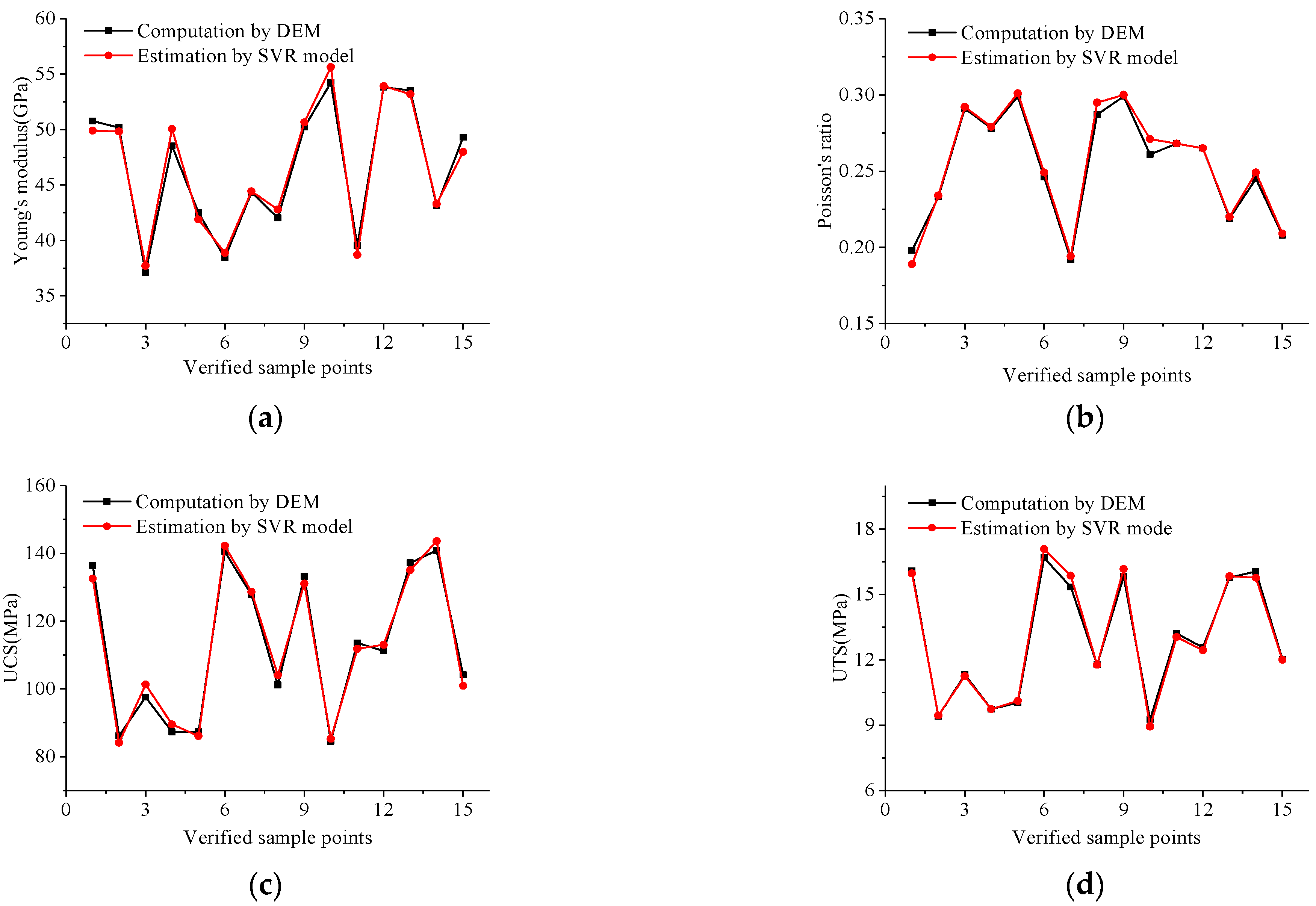
3.4. Approximation Model Technique

Generally, it should repeatedly use the computations for the forward problem during parameter identification, which may perform thousands of numerical calculations and then result in high costs. For the purpose of improving computational efficiency, the approximation model method was employed to substitute the real numerical calculations. Among the many approximation models, the support vector regression (SVR) model was adopted due to the strong capability for processing nonlinear problems, its high accuracy with a small number of samples, and its fine stability [32]. The Latin hypercube design (LHD) method [33], which is a widely used design of experiment (DOE) method and a space-filling design method based on a constrainedly stratified sampling, is used to generate the samples to construct the SVM model.

To construct a reliable approximation model, 30 samples for input parameter vector $x$ were generated in the inverse space by the LHD method and the corresponding computational responses $y_j(x),j=1,\dots ,4$ were obtained by performing DEM calculations under uniaxial compression and Brazilian splitting conditions, as listed in

Table 3. Samples by LHD method and corresponding computational responses.

Number	$\mathbf{Input}\mathbf{Parameter}{\mathbf{x}}_{\mathit{i}}$			Computational Responses ${\mathit{y}}_{\mathit{i}}\left(\mathbf{x}\right)$
	$E_c$(GPa)	$k_n/k_s$	${\overline{\sigma }}_c$(MPa)	$E$ (GPa)	$\upsilon$	${\sigma }_c$ (MPa)	${\sigma }_t$ (MPa)
1	20.03	2.92	36.30	35.14	0.300	119.37	14.4
2	26.00	2.87	28.24	45.94	0.296	99.08	11.47
3	29.18	2.77	21.64	52.07	0.298	79.61	8.93
4	27.86	1.85	24.85	53.83	0.224	100.2	11.24
5	21.51	2.39	22.32	39.5	0.267	84.93	9.56
6	23.74	1.51	25.34	47.6	0.186	103.55	12.22
7	25.23	2.19	29.19	47.07	0.252	110.9	12.66
8	29.41	1.94	31.26	56.37	0.231	122.75	13.91
9	21.18	1.77	29.93	41.14	0.214	116.3	13.62
10	28.99	1.83	38.62	56.04	0.221	145.69	17.27
11	27.61	2.13	30.40	51.91	0.247	117.2	13.34
12	24.09	1.67	39.03	47.38	0.205	146.03	18.07
13	21.84	2.41	32.42	39.93	0.268	115.52	13.55
14	24.95	2.23	39.49	46.26	0.257	141.31	16.89
15	25.55	2.62	23.58	46.2	0.282	86.47	9.8
16	20.80	2.68	34.82	37.16	0.288	119.87	14.24
17	26.94	2.51	26.04	48.77	0.277	97.78	10.9
18	22.09	1.56	33.35	44.08	0.193	130.77	15.84
19	24.59	1.64	35.87	48.65	0.201	137.11	16.87
20	26.03	1.97	21.24	49.63	0.232	86.87	9.47
21	22.58	2.27	24.20	41.71	0.258	92.09	10.38
22	23.08	2.57	23.27	41.79	0.279	85.65	9.7
23	27.27	2.06	32.98	51.43	0.243	125.93	14.45
24	22.90	2.84	37.65	40.45	0.297	128.38	15.17
25	28.64	2.73	26.76	51.15	0.289	97.3	11.02
26	29.81	2.99	37.01	52.15	0.303	125.06	14.73
27	28.11	2.30	34.40	51.81	0.260	127.06	14.61
28	23.48	2.02	20.22	44.53	0.237	81.45	8.96
29	26.52	1.73	31.51	51.86	0.211	123.04	14.55
30	20.45	2.47	27.65	37.08	0.272	100.86	11.53

.

Given the four computational responses obtained from DEM calculations, four SVR approximation models ${\tilde{y}}_j(x),j=1,\dots ,4$ were constructed. For verifying the accuracy of these approximation models, another 15 random samples in inverse spaces of inversed parameters were used to estimate the responses based on these constructed approximation models and then the results were compared with the corresponding results by DEM calculations, as shown in

Table 4. 15 random samples for verifying the SVR models.

Number	Input Parameter ${\mathbf{x}}_{\mathit{i}}$
	${\mathit{E}}_{\mathit{c}}\left(\mathbf{GPa}\right)$	${\mathit{k}}_{\mathit{n}}/{\mathit{k}}_{\mathit{s}}$	${\overline{\mathit{\sigma }}}_{\mathit{c}} \left(\mathbf{MPa}\right)$
1	25.67	1.62	34.20
2	26.37	1.97	21.07
3	20.90	2.75	27.67
4	26.86	2.53	23.18
5	24.16	2.91	24.70
6	20.48	2.10	38.20
7	22.21	1.55	32.23
8	23.56	2.69	28.55
9	28.56	2.89	39.27
10	29.25	2.27	21.44
11	21.67	2.42	31.62
12	29.36	2.37	29.66
13	27.77	1.82	35.00
14	22.94	2.08	36.83
15	25.18	1.71	25.91

and Figure 10. It can be found that the estimated responses by the SVR models were in good agreement with those from the DEM calculations; this indicated that the constructed approximation models were available and reliable.

3.5. Micro Multi-Objective Genetic Algorithm (µMOGA)

Based on the approximation models, a multi-objective optimization problem formulated in Equations (1) and (2) should be updated and specifically expressed as

$$Min\left\{\begin{array}{cc}{f}_1(x),& f_2(x)\end{array}\right\}$$

(3)

$$f_1{(x)}_{\mathrm{uniaxial}}={\displaystyle \sum _{j=1}^3\frac{\left|{\tilde{y}}_j^{}(x)-y_j^{ex}\right|}{y_j^{ex}}},f_2{(x)}_{\mathrm{brazilian}}=\frac{\left|{\tilde{y}}_4^{}(x)-y_4^{ex}\right|}{y_4^{ex}}$$

(4)

$$\begin{gathered} \mathrm{s}.\mathrm{t}.20\mathrm{MPa}\le E_c\le 30\mathrm{MPa} \\ 1.5\le k_n/k_s\le 3 \\ 20\mathrm{MPa}\le {\overline{\sigma }}_c\le 40\mathrm{MPa} \end{gathered}$$

(5)

where the inversed parameters vector $x=\left[E_c,K_n/K_s,{\overline{\sigma }}_c\right]$, the responses $y=\left[E,\nu ,{\sigma }_c,{\sigma }_t\right]$, the responses from the SVR model ${\tilde{y}}_j(x)$, and the responses from experiment $y_j^{ex}\mathrm{j}=1,\dots ,4$.

In this study, the micro-multi-objective genetic algorithm (µMOGA) [34] was utilized to solve this optimization problem. This algorithm has been validated to be an efficient multi-objective optimization method and has a small population size. In this algorithm, a non-dominated sorting and a crowded-comparison technique were adopted to classify the non-dominated levels and assigned fitness of each individual. Furthermore, it has a fine convergent performance and efficiency. In this work, the size of the population and the maximal generation used as the stopping criterion are set to 5 and 160 for µMOGA, respectively.

4. Results and Discussion

4.1. Results

Using the above multi-objective parameter identification technique, the Pareto optimal points of the inversed parameters were obtained through the proposed method after 223 point evaluations, as shown in Figure 11. If the approximation model had not been used in this method, the Pareto optimal points could be obtained by µMOGA after more than 4000 point evaluations. This indicates that the proposed method for parameter identification has good efficiency. Additionally, the four optimized parameter sets A, B, C, and D, which are closest to the line with 45°, are selected to be the initial identification results, as listed in

Table 5. Initial identification results.

Parameters	A	B	C	D
$E_c$ (GPa)	23.3	20.9	21.7	22.2
$k_n/k_s$	2.43	2.09	2.23	2.19
${\overline{\sigma }}_c$ (MPa)	32.5	33.4	34.5	32.5
$f_1{(x)}_{\mathrm{uniaxial}}$	0.258	0.224	0.196	0.175
$f_2{(x)}_{\mathrm{brazilian}}$	0.113	0.118	0.128	0.141

.

Then, the DEM calculations with these parameter sets were carried out to verify these results. Simultaneously, the corresponding values of the objective function were obtained by using Equation (4), as listed in

Table 6. Verification results for parameter identification.

Responses	A	B	C	D	Experiment
$E$(GPa)	42.3	39.3	40.4	40.4	41.5
$\nu$	0.248	0.244	0.249	0.249	0.23
${\sigma }_c$ (MPa)	117.2	125.5	125.2	115.4	138.8
${\sigma }_t$ (MPa)	10.47	10.51	10.66	10.78	9.5
$f_1{(x)}_{\mathrm{uniaxial}}$	0.254	0.213	0.209	0.194
$f_2{(x)}_{\mathrm{brazilian}}$	0.102	0.107	0.122	0.135

. It can be found that the values of $f_1{(x)}_{\mathrm{uniaxial}}$ and $f_2{(x)}_{\mathrm{brazilian}}$ listed in Table 6 are very close to those listed in Table 5, which further indicates that the construction of the SVR models in Section 3.4 have a fine accuracy. It also can be found that the computational responses of individual B have a good consistency with the experimental data and the total relative error is smaller compared with the others. Furthermore, the material fractures of the DEM calculation from individual B under the uniaxial compression and Brazilian splitting tests coincide with those from the experiments, as shown in Figure 12 and Figure 13. Consequently, the parameter values of individual B are considered as the inversed results for the three microparameters.

4.2. Validation

The validation for the inversed result is performed by DEM calculation under the three-point bending test. Firstly, according to the three-point bending test, the corresponding DEM model is established, as shown in Figure 14. In this model, the basic model parameters are the same as those in Section 3.2 and the parameter values of individual B are utilized. The boundary condition and loading are consistent with the experiment.

The result of the DEM calculation under the three-point bending test is given in

Table 7. Comparison of discrete element simulation results with experimental results.

Response	DEM Calculation	Experiment	Relative Error
$K_{IC}$ (MPa·m1/2)	1.152	1.057	8.98%

. The computational response is very close to the experimental response and the relative error is 8.98%. Then, the fracture from the DEM calculation is shown in Figure 15, which compared with the experimental measurement. It can be found that the DEM simulation agrees well with the experiment. These results validate that the inversed results based on the present multi-objective identification technique are effective and reliable.

5. Conclusions

In this work, a multi-objective identification approach is proposed to determine the DEM microparameters for brittle materials. This approach is combined with different kinds of experiments, numerical calculations, and multi-objective optimization algorithms. In this method, parameter identification is converted to solve a multi-objective optimization problem, which aims to minimize the relative deviations between the responses from the DEM calculation and those from the experiments. During the identification process, the uniaxial compressive test and Brazilian splitting test are directly used to determine the parameters and the three-point bending test is used to validate the identified results. Furthermore, a sensitivity analysis is carried out to obtain the inversed variables and ensure the inversed parameters are sensitive to the responses. The SVR approximation technique combined with LHD is utilized to construct an approximation model to improve the computational efficiency. µMOGA is employed as an inverse operator to solve the multi-objective optimization problem. Finally, the DEM microparameters for granite are successfully identified by the developed inverse method. The results indicate that the presented multi-objective identification method provides a useful tool for identifying DEM microparameters for brittle materials with fine accuracy and efficiency, and it can be applied to parameter identification of other materials.

References

1. Cundall, P.A.; Strack, O.D.L. A discrete numerical model for granular assemblies. Géotechnique 1979, 29, 47–65. [Google Scholar] [CrossRef]
2. Sinnott, M.D.; Cleary, P.W. The effect of particle shape on mixing in a high shear mixer. Comput. Part. Mech. 2016, 3, 477–504. [Google Scholar] [CrossRef]
3. Alian, M.; Ein-Mozaffari, F.; Upreti, S.R. Analysis of the mixing of solid particles in a plowshare mixer via discrete element method (DEM). Powder Technol. 2015, 274, 77–87. [Google Scholar] [CrossRef]
4. Müller, P.; Tomas, J. Simulation and calibration of granules using the discrete element method. Particuology 2014, 12, 40–43. [Google Scholar] [CrossRef]
5. Shen, W.; Zhao, T.; Dai, F.; Jiang, M.; Zhou, G.G. DEM analyses of rock block shape effect on the response of rockfall impact against a soil buffering layer. Eng. Geol. 2019, 249, 60–70. [Google Scholar] [CrossRef]
6. Van Wyk, G.; Els, D.; Akdogan, G.; Bradshaw, S.; Sacks, N. Discrete element simulation of tribological interactions in rock cutting. Int. J. Rock Mech. Min. Sci. 2014, 65, 8–19. [Google Scholar] [CrossRef]
7. Wang, Y.; Tonon, F. Discrete Element Modeling of Drop Tests. Rock Mech. Rock Eng. 2012, 45, 863–869. [Google Scholar] [CrossRef]
8. Karampinos, E.; Hadjigeorgiou, J.; Hazzard, J.; Turcotte, P. Discrete element modelling of the buckling phenomenon in deep hard rock mines. Int. J. Rock Mech. Min. Sci. 2015, 80, 346–356. [Google Scholar] [CrossRef]
9. Espada, M.; Muralha, J.; Lemos, J.V.; Jiang, Q.; Feng, X.-T.; Fan, Q.; Fan, Y. Safety Analysis of the Left Bank Excavation Slopes of Baihetan Arch Dam Foundation Using a Discrete Element Model. Rock Mech. Rock Eng. 2018, 51, 2597–2615. [Google Scholar] [CrossRef]
10. Scholtès, L.; Donzé, F.-V. A DEM model for soft and hard rocks: Role of grain interlocking on strength. J. Mech. Phys. Solids 2013, 61, 352–369. [Google Scholar] [CrossRef]
11. Fakhimi, A. Application of slightly overlapped circular particles assembly in numerical simulation of rocks with high friction angles. Eng. Geol. 2004, 74, 129–138. [Google Scholar] [CrossRef]
12. Tarantola, A. Inverse Problem Theory and Methods for Model Parameter Estimation; Society for Industrial and Applied Mathematics (SIAM): Philadelphia, PA, USA, 2005. [Google Scholar] [CrossRef] [Green Version]
13. Aster, R.; Borchers, B. Parameter Estimation and Inverse Problem; Elsevier: Amsterdam, The Netherlands, 2013. [Google Scholar]
14. Han, X.; Liu, G.R. Computational Inverse Technique for Material Characterization of Functionally Graded Materials. AIAA J. 2003, 41, 288–295. [Google Scholar] [CrossRef]
15. Horabik, J.; Molenda, M. Parameters and contact models for DEM simulations of agricultural granular materials: A review. Biosyst. Eng. 2016, 147, 206–225. [Google Scholar] [CrossRef]
16. Benvenuti, L.; Kloss, C.; Pirker, S. Identification of DEM simulation parameters by Artificial Neural Networks and bulk experiments. Powder Technol. 2016, 291, 456–465. [Google Scholar] [CrossRef]
17. Coetzee, C. Review: Calibration of the discrete element method. Powder Technol. 2017, 310, 104–142. [Google Scholar] [CrossRef]
18. Do, H.; Aragón, A.M.; Schott, D.L. A calibration framework for discrete element model parameters using genetic algorithms. Adv. Powder Technol. 2018, 29, 1393–1403. [Google Scholar] [CrossRef]
19. Yoon, J. Application of experimental design and optimization to PFC model calibration in uniaxial compression simulation. Int. J. Rock Mech. Min. Sci. 2007, 44, 871–889. [Google Scholar] [CrossRef]
20. Tawadrous, A.S.; DeGagné, D. Prediction of uniaxial compression PFC3D model micro-properties using artificial neural net-works. Int. J. Numer. Anal. Methods Geomech. 2009, 33, 1953–1962. [Google Scholar] [CrossRef]
21. Kazerani, T. Effect of micromechanical parameters of microstructure on compressive and tensile failure process of rock. Int. J. Rock Mech. Min. Sci. 2013, 64, 44–55. [Google Scholar] [CrossRef]
22. Do, H.Q.; Aragón, A.M.; Schott, D.L. Automated discrete element method calibration using genetic and optimization algo-rithms. EPJ Web Conf. EDP Sci. 2017, 140, 15011. [Google Scholar] [CrossRef]
23. De Simone, M.; Souza, L.M.; Roehl, D. Estimating DEM microparameters for uniaxial compression simulation with genetic programming. Int. J. Rock Mech. Min. Sci. 2019, 118, 33–41. [Google Scholar] [CrossRef]
24. Marler, R.T.; Arora, J.S. Survey of multi-objective optimization methods for engineering. Struct. Multidiscip. Optim. 2004, 26, 369–395. [Google Scholar] [CrossRef]
25. Chiandussi, G.; Codegone, M.; Ferrero, S.; Varesio, F.E. Comparison of multi-objective optimization methodologies for engineering applications. Comput. Math. Appl. 2012, 63, 912–942. [Google Scholar] [CrossRef] [Green Version]
26. Chen, G.; Han, X.; Liu, G.; Jiang, C.; Zhao, Z. An efficient multi-objective optimization method for black-box functions using sequential approximate technique. Appl. Soft Comput. 2012, 12, 14–27. [Google Scholar] [CrossRef]
27. Milani, A.; Dabboussi, W.; Nemes, J.; Abeyaratne, R. An improved multi-objective identification of Johnson–Cook material parameters. Int. J. Impact Eng. 2009, 36, 294–302. [Google Scholar] [CrossRef]
28. Papon, A.; Riou, Y.; Dano, C.; Hicher, P.-Y. Single-and multi-objective genetic algorithm optimization for identifying soil parameters. Int. J. Numer. Anal. Methods Géoméch. 2011, 36, 597–618. [Google Scholar] [CrossRef] [Green Version]
29. Potyondy, D.O.; Cundall, P.A. A bonded-particle model for rock. Int. J. Rock Mech. Min. Sci. 2004, 41, 1329–1364. [Google Scholar] [CrossRef]
30. Jiang, S.; Li, X.; Tan, Y.; Liu, H.; Xu, Z.; Chen, R. Discrete element simulation of SiC ceramic with pre-existing random flaws under uniaxial compression. Ceram. Int. 2017, 43, 13717–13728. [Google Scholar] [CrossRef]
31. Yang, B.; Jiao, Y. A study on the effects of micro-parameters on macro-properties for specimens created by bonded particles. Eng. Comput. 2006, 23, 607–631. [Google Scholar] [CrossRef]
32. Clarke, S.M.; Griebsch, J.H.; Simpson, T.W. Analysis of Support Vector Regression for Approximation of Complex Engineering Analyses. J. Mech. Des. 2004, 127, 1077–1087. [Google Scholar] [CrossRef]
33. Peter, G.; Bradley, J. Optimal Design of Experiments: A Case Study Approach; Wiley: New York, NY, USA, 2011. [Google Scholar]
34. Liu, G.P.; Han, X. A micro multi-objective genetic algorithm for multi-objective optimizations. In Proceedings of the Fourth China-Japan-Korea Joint Symposium on Optimization of Structural and Mechanical Systems, Kunming, China, 6–9 November 2006. [Google Scholar]
Figure 1. Flowchart of multi-objective identification technique.
Crystals 12 00387 g001
Figure 2. Experimental samples: (a) Uniaxial compression test sample. (b) Brazilian splitting test sample. (c) Three-point bending test sample.
Crystals 12 00387 g002
Figure 3. Uniaxial compression experimental device.
Crystals 12 00387 g003
Figure 4. Brazilian splitting experimental device.
Crystals 12 00387 g004
Figure 5. Three-point bending experiment information. (a) Schematic diagram; (b) Specific device.
Crystals 12 00387 g005
Figure 6. Stress–strain curves measured from experiments. (a) Uniaxial compression tests; (b) Brazilian splitting tests.
Crystals 12 00387 g006
Figure 7. Force–displacement curves measured from three-point bending tests.
Crystals 12 00387 g007
Figure 8. Discrete element model: (a) Uniaxial compression test model. (b) Brazilian splitting test model.
Crystals 12 00387 g008
Figure 9. Sensitivity analysis for unknown microparameters in uniaxial compression test. (a) Parameter E c ; (b) Parameter K n / K s ; (c) Parameter σ ¯ c ; (d) Parameter τ ¯ c ; and (e) Parameter μ .
Crystals 12 00387 g009
Figure 10. The verification for SVR models. (a) Yong’s modulus; (b) Poisson’s ratio; (c) UCS; (d) UTS.
Crystals 12 00387 g010
Figure 11. Obtained Pareto optimal points by the present method.
Crystals 12 00387 g011
Figure 12. The material fractures under uniaxial compressive test. (a) DEM calculation with individual B; (b) Experiment.
Crystals 12 00387 g012
Figure 13. The material fractures under Brazilian splitting test. (a) DEM calculation with individual B; (b) Experiment.
Crystals 12 00387 g013
Figure 14. A DEM model for three-point bending test.
Crystals 12 00387 g014
Figure 15. Comparison of simulated and experimental destruction result for three-point bending experiment. (a) DEM calculation result; (b) Experimental result.
Crystals 12 00387 g015