Phase Diagram Determination and Process Development for Continuous Antisolvent Crystallizations

Abstract

The development of an antisolvent crystallization process requires the construction of an accurate phase diagram for this ternary system of compound, solvent and antisolvent, preferably as a function of temperature. This study gives an efficient methodology to systematically determine such antisolvent phase diagrams, exemplified with four model compounds: Sodium bromate, DL-Asparagine Monohydrate, Mefenamic acid and Lovastatin. Using clear point temperature measurements, single solvent and mixed solvent-antisolvent solubilities are obtained, showing strongly non-linear solubility dependencies as well as more complex solubility behaviour as a function of antisolvent fraction. A semi-empirical model equation is used to describe the phase diagram of the antisolvent crystallization system as a function of both temperature and antisolvent fraction. The phase diagram model then allows for the identification of condition ranges for optimal productivity, yield, and suspension density in continuous antisolvent crystallization processes.

1. Introduction

The access to accurate solubilities of pharmaceutical compounds sets the foundations towards the optimal design and optimization of crystallization processes [1,2]. Although there are methods developed to determine the solubility using computational methods, such as the SAFT-γ MIE approach [3], they are not accurate enough to rely on in the crystallization process design. It is thus required to experimentally determine the solubility to have access to an accurate phase diagram, enabling a reliable crystallization process development, but also to satisfy regulatory approval conditions [4,5,6]. While solubility data of pure compounds in single solvents is relatively easily accessible nowadays using commercially available equipment and standardized methods [7], solid solubilities in more complex systems such as binary solvent mixtures are much less easy to obtain [8,9,10,11]. Solid solubilities in binary solvent mixtures are needed to build phase diagrams to use in the antisolvent crystallization process development [12,13]. Antisolvent crystallization is based on the substantial and non-linear dependence of the solubility upon increasing the antisolvent fraction, a solubility decrease that should be substantially more than the concentration decreases due to the dilution because of the antisolvent addition, as shown in Figure 1 [1]. Antisolvent crystallization can only take place if, at a specific antisolvent fraction, the solubility (the solid line in Figure 1) drops below the diluted concentration (the dashed line in Figure 1). Continuous antisolvent crystallization can be performed in various process configurations using Plug Flow Tubes [14,15,16,17,18] or Continuously Stirred Tanks (CST) [13,19,20,21]. One of the possible continuous antisolvent CST crystallization configurations is shown next to the phase diagram in Figure 1.

In order to establish the phase diagram in antisolvent crystallization process development, a common method used is the gravimetric method, in which a suspension is equilibrated and the solution concentration is determined at a specific temperature [11,16,22,23]. Work by Reus et al. [7] showed a variation of this equilibrium method, utilizing solvent addition to a suspension in a mixed solvent antisolvent system at constant temperature in order to dissolve the suspended crystals and obtain the antisolvent fraction at which the overall concentration equals the saturation concentration. Alongside these methods, spectroscopic methods [24] are used to determine the solubility in equilibrated mixed solvent suspensions such as in the case of sulfadiazine [25]. Although effective, the constant temperature method commonly used takes substantial laboratory effort and time.

The temperature variation method, in which the temperature of a suspension is slowly increased until the temperature dependent solubility matches the overall sample composition and all crystals dissolve [26], has become more widely used. In this method, the saturation temperature is approximated by the clear point temperature, the temperature at which, upon increasing the temperature of a suspension, the suspension turns into a clear solution. This method has been utilized in many single solvent systems to establish single solvent solubility data. However, its applicability has not yet been widely used for the process of establishing mixed solvent solubility data, as temperature is introduced as an additional variable, next to compound concentration and antisolvent fraction, increasing the complexity of the analysis. One previous example of the use of the temperature variation method for such a complex system related to antisolvent crystallization is reported by Vellema et al. [27] describing the solubility of lorazepam at varying levels of glucose solution, in order to determine the correct operating window to prevent recrystallization of lorazepam mixed solution during infusion in intensive care units.

The aim of this work is to outline a systematic approach to accurately obtain temperature-dependent phase diagrams for the development of antisolvent crystallization processes. For four model systems, the phase diagram for antisolvent crystallization is determined as a function of temperature and antisolvent fraction. From the solubility data, a solubility model is established. The model is then used to propose operation conditions for a continuous antisolvent crystallization process identifying the most optimal region in terms of antisolvent fraction and temperature to achieve a productivity P, yield Y and suspension density r within specifications.

2. Materials and Methods

The molecular structures of the model compounds are shows in Figure 2. Lovastatin (LOV) was supplied from Molekula (>98%, Darlington), DL-Asparagine Monohydrate (ASN), Sodium Bromate (NaBrO₃) and Mefenamic Acid (MFA) were obtained from Sigma Aldrich (>99%). All compounds were used as received. For solution preparation, acetone (99%) and ethanol (99%) were obtained from VWR International. The distilled and filtered water was obtained from an in-house Millipore Systems setup.

For the clear point measurements a known amount of the crystalline compound was added to a standard HPLC vial. Then, about 1 mL of a solvent/antisolvent mixture with known antisolvent mass fraction x_AS was pipetted into the vial from a larger volume of prepared solvent/antisolvent mixture stock solution. These vials were weighed before and after addition of solvent mixture to exactly determine the mass of solvent mixture added. The composition of the sample is denoted by the (solute-free) antisolvent mass fraction x_AS and the solute concentration C in units of g/g-solvent mixture. Due to its low solubility, we chose to neglect the influence on the sample antisolvent fraction of the amount of water in the DL-Asn.H₂O crystals.

The Crystal16 Multiple Reactor Setup (Technobis Crystallization Systems) was used to determine the clear point temperature of the prepared samples. The clear point temperature is the temperature at which, upon heating, a suspension turns into a clear solution. The clear point temperature of the samples was determined in triplicate using automated temperature profiles. First, the suspension was dissolved by keeping the sample at a temperature well above the saturation temperature for 30 min. Then, the sample was recrystallized by cooling down to a temperature well below the saturation temperature and keeping the sample at that temperature for at least 30 min. Finally, three temperature cycles were performed to determine 3 clear point temperatures in the heating part of the temperature cycle. A single temperature cycle consisted of a heating part in which the suspension was heated with a heating rate of 0.2 °C/min, a constant high temperature part of 30 min, a cooling part in which the clear solution was cooled with a cooling rate of 0.4 °C/minute, and a constant low temperature part of 30 min. The average of the 3 clear point measurements was assumed to be equal to the saturation temperature of the sample concentration C at the antisolvent fraction x_AS in the vial.

Occasionally, samples displayed larger than 1 °C difference between clear point temperatures measured in subsequent cycles and these measurements were then discarded, and fresh samples were used in a re-run. This deviation in clear points was usually coinciding with crowning of crystals just above the liquid level in the sample vials. The occurrence of crowning substantially decreased when the stirring rate in the constant high temperature region of the temperature profile was increased.

Due to known issues of lovastatin degrading over time in solutions at higher water content, the total experimental time experienced by each sample containing lovastatin was kept smaller than 24 h. There were no observations of large decreases in subsequent clear point temperatures of the same sample, indicating that the degradation of lovastatin is negligible.

The procedure was slightly adapted for MFA measurements due to the polymorphic nature of MFA to remove the impact of potential nucleation of the undesired form during the dissolution–recrystallization cycling. Instead of 3, only a single measurement was obtained for a sample, using the initial suspension in the vial without the initial dissolution step. Vials filled with pure ethanol were used to calibrate the transmission of light in the Crystal16 equipment for a clear solution. Subsequently, the prepared vials containing MFA slurries with the original raw material (Form 1) in ethanol–water mixtures were added to the machine and a single temperature cycle was performed. The clear point temperature at which 100% light transmission was reached was taken as the saturation temperature of the sample. A larger number of measurement samples were prepared for this model compound.

Fitting of experimental data was done using the MatLab Curve Fitting tool and by using the scipy.optimize curve_fit routine within Python.

3. Results

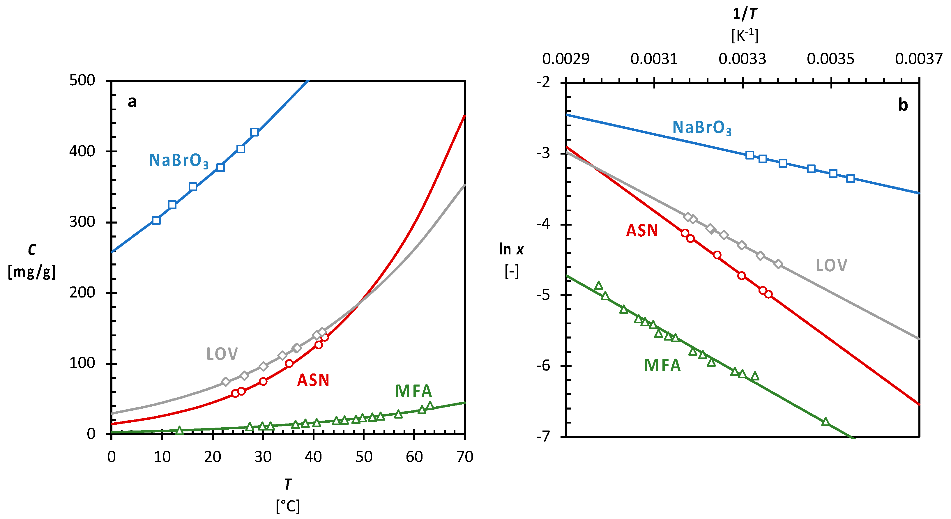
3.1. Single Solvent Solubility

Figure 3a displays the measured temperature-dependent solubilities of NaBrO₃ in water, DL-Asn.H₂O in water, MFA in ethanol and LOV in acetone. Each system shows a strong temperature dependence of the solubility.

Sodium bromate (NaBrO₃, Figure 2) is a water-soluble salt. Dissolved in water, it is achiral but it crystallizes in the chiral space group P2₁3 [28]. Similar to some other sodium salts [29] the solubility of NaBrO₃ in water is high, 367 mg/g at 25 °C, and it increases with temperature to 505 mg/g at 40 °C (Figure 3a). As NaBrO₃ is a salt with a high solubility in water and a low solubility in ethanol, it can be produced by antisolvent crystallization from solutions in water using ethanol as an antisolvent [21].

Lovastatin (LOV) from the statin family has a molecular structure (Figure 2) with several chiral centres and it is used in the treatment of high cholesterol and cardiovascular disease. It does not appear to have any known polymorphs. The solubility of LOV in acetone is ranging from 80 to 180 mg/g between 20 and 40 °C (Figure 3a). The very low solubility of LOV in water in comparison to acetone makes it an interesting model compound for antisolvent crystallization [30].

The racemic asparagine monohydrate (ASN, Figure 2) is a non-essential amino acid and is known to crystallize as a conglomerate forming system. Asparagine monohydrate has a solubility in water of around 80 to 180 mg/g between 20 and 40 °C (Figure 3a). The solubility of ASN is known to decrease with the antisolvent ethanol fraction while ASN recrystallizes as the anhydrous form at sufficiently large ethanol fractions [7].

Mefenamic acid (MFA, Figure 2) is a member of the anthranilic acid derivatives of non-steroidal anti-inflammatory drugs (NSAIDs), used for the treatment of mild and moderate pains. It is not widely used compared to other NSAID due to its higher costs. MFA is known to crystallize in three polymorphic forms [31,32]. The solubility of MFA in ethanol is the lowest of the measured pure solvent systems, with solubilities between 10 and 42 mg/g at temperatures ranging from 25 to 60 °C (Figure 3a). MFA has a very low solubility in water, similar to other NSAID on the market, making water a potential antisolvent.

The ideal solubility x_id is usually described as a function of temperature T using only two solid state properties: melting temperature T_m and heat of fusion ΔH (kJ mol⁻¹) [33]:

$$x_{id}=\exp \left(-\frac{\Delta H}{R}\left(\frac{1}{T}-\frac{1}{T_m}\right)\right)$$

(1)

with the molar gas constant R. Due to non-ideality in the solution, the ideal solubility can substantially deviate from the measured solubilities. Often, Equation (2), the linearized form of Equation (1), gives a good fit to experimental data within a sufficiently narrow temperature region using the parameters A and B as fitting parameters:

$$\ln x=\frac{A}{T}+B$$

(2)

The parameters A and B can be determined from a linear fit of Equation (2) to the experimental data in the plot of $\ln x$ versus 1/T. Equation (2) describes well the measured solubilities in (Figure 3b) within the measured temperature region.

3.2. Solubility in Solvent/Antisolvent Mixtures

Figure 4a,c,e,g display the temperature dependent solubility for all model compounds obtained at specific anti-solvent fractions x_AS. In all instances, at a constant antisolvent fraction x_AS, the solubility increases with temperature. The solubility at a particular antisolvent fraction x_AS can well be described by Equation (2) as shown by the dashed lines in the right graphs of Figure 4b,d,f,h.

For NaBrO₃, at a specific temperature the solubility reduces non-linearly as a function of the antisolvent fraction x_AS (Figure 4a,b). When going from x_AS = 0 to 0.1 at 30 °C the solubility drops 51% from 366 to 181 mg/g. The solubility drops further to 94 mg/g going to x_AS = 0.2, and at x_AS = 0.5 it has decreased by 95% from its solubility in pure water. This trend of a strong non-linear solubility decrease as a function of antisolvent is consistent with the preferred antisolvent phase diagram behaviour for systems with optimal antisolvent crystallization potential [34,35]. ASN and MFA show similar behaviour with the solubilities decreasing as a function of antisolvent fraction (Figure 4c–f). At 30 °C the solubility shows, respectively, a 40% and 37% drop, going from x_AS = 0 to 0.1. The solubility of ASN, for instance, drops from 75 mg/g at x_AS = 0 to 45 mg/g at x_AS = 0.1 at 30 °C for DL-Asn.H₂O.

Conversely, LOV in ethanol–water shows, at small antisolvent fractions, an increase in solubility compared to the solubility in absence of antisolvent (Figure 4g,h). Going from x_AS = 0 to 0.05 at 30 °C, the solubility increases from 98 to 122 mg/g, a 26% increase. As the antisolvent fraction increases further, the solubility decreases. At x_AS = 0.1 the solubility reduces to 98 mg/g and it reduces to below its pure system concentration at x_AS = 0.2. At x_AS = 0.5 the solubility has further decreased to 4.6 mg/g. Such a solubility maximum at a specific antisolvent fraction may be a complex combination of molecular, thermodynamic, and entropic effects. For instance, antisolvent molecules of water may shield unfavourable polar parts of the complex molecule LOV to enable a better interaction of the solvent molecules of acetone with LOV, increasing the solubility. Several systems are reported to exhibit solubility behaviour similar to LOV in solvent–antisolvent mixtures [24,25,31].

3.3. Antisolvent Crystallization Phase Diagrams

For the system of NaBrO₃ in water/ethanol, the fitted parameters A and B to Equation (2) at each antisolvent fraction are shown in Figure 5. The parameters A and B change substantially with the antisolvent fraction x_AS. The other systems show a similar behaviour. Utilizing the observed behaviour of the solubility as a function of temperature and antisolvent fraction a single empirical equation is proposed based on Equation (2), in which the antisolvent fraction dependence is of parameters A and B is captured by simple polynomials:

$$\ln x=\left({\displaystyle \sum }_{i=0}^n{a}_i{x}_{AS}^i\right)\frac{1}{T}+{\displaystyle \sum }_{i=0}^n{b}_i{x}_{AS}^i$$

(3)

The goodness of the fit for the model is determined for each system using Equation (4) for the relative standard deviation σ_z in % with N the total number of experimental points used, with z = x or lnx:

$${\sigma }_z=100\times \sqrt{\frac{{\sum }_{i=1}^N{\left(\frac{z_i-z_{pred}}{z_i}\right)}^2}{N-1}}$$

(4)

An σ_lnx = 1% means that the resulting parameters describe the lnx data with on average 68% of the datapoints having less than a 1% deviation from the model lnx value.

The simple model of Equation (3) allows us to fit all experimental data for a specific system and the fitted parameters are shown in

Table 1. Fitting parameters and their standard errors obtained from the model Equation (3) using the entire dataset for a combination of compound, solvent and antisolvent. The relative standard deviations σ_lnx and σ_x from Equation (4) for each system are also provided.

Compound	NaBrO3	ASN	MFA	LOV
Solvent	Water	Water	Ethanol (EtOH)	Acetone (AcO)
Antisolvent	Ethanol (EtOH)	Ethanol (EtOH)	Water	Water
N	22	27	65	39
n	2	1	1	2
a0 × 10−3	−1.26 ± 0.2	−4.84 ± 0.16	−3.50 ± 0.09	−2.80 ± 0.36
a1 × 10−3	−10.8 ± 1.6	−1.40 ± 0.47	−2.12 ± 0.64	−8.30 ± 5.10
a2 × 10−3	14.8 ± 2.8			12.6 ± 11.2
b0	1.12 ± 0.55	11.5 ± 0.5	5.44 ± 0.27	5.0 ± 1.2
b1	31.4 ± 5.4	0.0 ± 1.5	0.75 ± 1.97	28.8 ± 16.5
b2	−48.9 ± 9.5			−60.0 ± 36.2
σlnx	0.8%	0.7%	0.8%	1.7%
σx	3.3%	3.7%	5.1%	8.9%

. The order n of the polynomial is chosen to be the 0 ≤ n ≤ 2 for which the relative standard deviation σ_lnx is below 1% or else the smallest. We chose to fit lnx rather than x, but also give the value for σ_x in Table 1 to show how well the parameters describe solubility fraction x.

The model with n = 2 describes the NaBrO₃ system well, with a standard deviation σ_lnx = 0.8%, which means that on average 68% of the experimental lnx values deviate less than 0.8% from those predicted by the model. The standard deviation in the mole fraction x is slightly larger, σ_x = 3.3%, as the fit was performed on lnx rather than on x. While the NaBrO₃ system needs six parameters to be described well, the systems of ASN and MFA can do with four, using n = 1 in Equation (3). The standard deviations of the ASN and MFA systems are, respectively, σ_lnx = 0.7% and 0.8%. Looking at the large relative standard error in parameter b₁ in Table 1, both systems can also be described using three rather than four parameters, with an antisolvent fraction independent B-parameter (b₁ = 0). The standard deviation using three parameters is not substantially increasing for both systems. For the LOV system, with the more complex antisolvent fraction dependent solubility behaviour, the model, using n = 2, performs reasonably with a σ_lnx = 1.7%. The ability of the model to capture the change in antisolvent and temperature is shown by the solid lines in the lnx—1/T diagrams in Figure 4.

The parameters in Table 1 can be used to construct an antisolvent crystallization phase diagram at constant temperature, where the solubility is shown as a function of the antisolvent fraction x_AS. Figure 6a,c,e,g show the antisolvent crystallization phase diagrams for all the systems constructed using the model at a specific temperature. The solubility decreases strongly linearly with increasing antisolvent fraction for the systems of NaBrO₃, ASN and MFA. For the LOV system, the increase of the solubility at low antisolvent fractions is clearly seen, while at a higher antisolvent fraction, the solubility sharply decreases with the antisolvent fraction. It is interesting to note that the solubility continues to decrease towards pure antisolvent (x_AS = 1), even for antisolvent fractions larger than the ones at which the solubilities were measured.

The determined phase diagrams are very helpful in the development of continuous antisolvent crystallization processes such as that in Figure 1.

3.4. Continuous Antisolvent Crystallization

The pharmaceutical industry has been increasingly adopting continuous manufacturing for both primary (drug substance) and secondary (drug product) processing. The use of continuous crystallization rather than batch-wise crystallization allows higher productivities and yields to be obtained, while allowing better control of critical quality attributes and reducing product variations, often seen from batch to batch [36]. A continuously stirred tank antisolvent crystallization process has continuous inlets of concentrated solution and of antisolvent as well as a continuous suspension outlet stream and is operated in a steady state in which, in principle, the suspension properties do not change over operation time (Figure 1).

In continuous antisolvent crystallization processes, the mixing of the pure antisolvent and the solution results in two effects, shown in the schematic in Figure 1. On the one hand, by adding an antisolvent the solubility C*(x_AS, T) decreases in the resulting mixture. This antisolvent fraction-dependent solubility at constant temperature is shown for all systems in Figure 6, calculated using the constructed phase diagram model. On the other hand, the addition of antisolvent dilutes the solution, decreasing the overall concentration in the mixed solution compared to the feed concentration C_F. The overall concentration C_M at a specific antisolvent x_AS fraction is a function of the feed concentration C_F and solute concentration C_AS in the antisolvent.

$$C_M\left(x_{AS}\right)=C_F-\left(C_F-C_{AS}\right)\frac{x_{AS}-x_{AS}^F}{x_{AS}^{AS}-x_{AS}^F}$$

(5)

Here we also account for the antisolvent fractions in the solution feed and antisolvent feed which might deviate from x_AS^F = 0 and x_AS^AS = 1, respectively. The dashed straight line in Figure 6 represents the dilution line C_M(x_AS) = C_F(1 − x_AS) for a process with a feed of solute in pure solvent, saturated at the process temperature (C_F = C*(x_AS^F = 0, T)), and a feed of pure antisolvent (C_AS = 0, x_AS^AS = 0) at the same temperature. Only at an antisolvent fraction at which the overall concentration C_M is higher than the solubility C* (the dilution line is above the solubility line), overall supersaturation is created and antisolvent crystallization can take place [37].

A continuous antisolvent crystallization at ambient pressure is determined by the operating conditions of temperate T, residence time τ and antisolvent fraction x_AS [38]. The operating temperature T in the crystallizer determines the solubility C*(x_AS, T) at the prevailing antisolvent fraction. In steady state, the antisolvent fraction x_AS in the crystallizer is constant and determined by the size of the antisolvent feed flow rate with respect to the sum of the feed flow rates. The residence time τ = v/v is defined as the average time molecules spend in the crystallizer and is determined by the crystallizer volume V and the flow rate v of the suspension leaving the crystallizer.

In continuous antisolvent crystallization process development, we can define three limiting process requirements such as in Figure 1, for yield Y, productivity P, and suspension density r. Long residence times allow the complete consumption of the supersaturation by the growing crystals and therefore a maximum product yield Y to be obtained. Then, we can use the equilibrium stage concept often used in the early stages of separation technology process development [39]. The maximum yield Y at a specific antisolvent fraction x_AS is then defined by the difference between overall concentration C_M(x_AS) and solubility C*(x_AS) at that antisolvent fraction, relative to the overall concentration:

$$Y\left(x_{AS}\right)=\frac{C_M\left(x_{AS}\right)-C^{*}\left(x_{AS}\right)}{C_M\left(x_{AS}\right)}$$

(6)

However, as the solubility C*(x_AS) is not zero, some solute remains in solution and creates a loss of potential product. The yield Y is related to the loss L = 1 − Y of product that remains dissolved in the solvent mixture. The loss of product needs to be as small as possible, and a maximum acceptable product loss can be defined, for example, as L_max = 0.1, in which case 10% of the incoming solute is not crystallized. The target minimum yield therefore is set to Y_min = 0.9.

If the crystallization kinetics are relatively fast, a comparatively short residence time may suffice to achieve a high productivity, the amount of product produced per unit of time and feed mass. The maximum productivity P at a specific antisolvent fraction x_AS is defined by the difference in overall concentration C_M and solubility C* at that antisolvent fraction and the residence time τ:

$$P\left(x_{AS}\right)=\frac{C_M\left(x_{AS}\right)-C^{*}\left(x_{AS}\right)}{\tau }$$

(7)

At a specific residence time, the maximum productivity therefore can be achieved at the antisolvent fraction at which the difference between overall concentration and solubility is the largest. A target minimum productivity of an economically viable chemical process leading can be regarded, for example, to be about P_min = 12 mg/g.hr. Since information on crystallization kinetics is usually not available during early stages of the process development, a lower limit of the residence time is not a priori known. However, if the residence time becomes too short, the maximum productivity will not be achieved as the solution concentration in the crystallizer will significantly deviate from the saturation concentration since the crystallization kinetics will not be fast enough to consume all supersaturation. We can assume that a reasonable residence time may be at τ = 0.5 hr, for which the crystals would need a linear growth rate of crystal faces of about 28 nm/s or an overall crystal growth rate of 3.3 μm/minute to arrive at a product size of about 100 μm, however, a suitable residence time should be based on experimental validation for a particular system.

The third limiting process requirement is set on the suspension density ρ, which is defined as the weight fraction of the crystallizer suspension occupied by the solid phase. This is calculated from the following equation, with the units for concentration in mg/g-solution:

$${\rho }_{}=\frac{C_M\left(x_{AS}\right)-C^{*}\left(x_{AS}\right)}{1000+C_M\left(x_{AS}\right)-C^{*}\left(x_{AS}\right)}$$

(8)

The more product crystallizes from the solution, the larger the suspension density. If the suspension density becomes too high, the suspension of crystals is hampered which would decrease the product quality. We assume that a suspension density of ρ_max = 0.2 is the upper limiting process requirement of a continuous antisolvent crystallization to maintain proper mixing and with it a good product quality.

The predicted yield Y, productivity $P$, and slurry density $\rho$ as a function of the antisolvent fraction x_AS are presented in Figure 6b,d,f,h for each system using a residence time τ = 0.5 h and a saturated feed at the process temperature T. The productivity of NaBrO₃ increases significantly from $x_{AS}$ = 0 up to $x_{AS}$ = 0.25 with a maximum productivity of 409 mg/g.hr (Figure 6a). At higher antisolvent fractions the productivity decreases again. The productivity is well above its minimum value P_min = 12 mg/g.hr for almost the entire x_AS region. The yield Y increases up to an antisolvent fraction of x_AS = 0.75 and a yield Y = 0.94, after which the yield drops to zero. The yield Y > Y_min = 0.9 in the antisolvent fraction region 0.5 < x_AS < 0.9. Even for this high drop in solubility the suspension density r < r_max remains low enough for all 0 < x_AS < 1. Considering productivity, yield, and suspension density the optimal antisolvent fraction region to perform this process is therefore 0.5 < x_AS < 0.9, indicated by the green arrow in Figure 6b.

The ASN system shows a similar behaviour for productivity P, yield Y and suspension density r, although productivity and suspension density are much lower than in the case of NaBrO₃ as the ASN solubility is much lower (Figure 6d). In this case the optimal antisolvent fraction is 0.5 < x_AS < 0.95. However, at these high antisolvent fractions it might well be that the anhydrate rather than the hydrate of ASN is formed within the process.

For the MFA system the solubility is even lower and therefore, at 20 °C, does not result in a productivity P > P_min in the entire range of antisolvent fraction (Figure 6f). By increasing the process temperature to 45 °C (Figure 6e, f), the productivity increases and P > P_min from x_AS = 0.09 to an antisolvent fraction slightly higher than x_AS = 0.65. At 45 °C, the yield Y > Y_min in the region 0.65 < x_AS < 0.85. The optimal antisolvent fraction is therefore around x_AS = 0.65 at which the yield is Y = 0.9 and productivity P = 12.67 mg/g.hr.

Because of the increasing solubility at smaller antisolvent fractions, the productivity and yield are zero below x_AS = 0.15 for the LOV system (Figure 6h). However, beyond that antisolvent fraction the solubility shows a huge drop to close to zero resulting in high productivities (0.2 < x_AS < 0.9) and yields (0.45 < x_AS < 0.99). This makes the optimal antisolvent fraction for continuous antisolvent crystallization to be 0.45 < x_AS < 0.9 as shown by the green arrow in Figure 6h.

4. Discussion

By applying the experimental methodology introduced here, antisolvent phase diagrams can be accurately determined across a range of solvent-antisolvent mixture compositions and temperatures. The methodology is based on measuring a number of clear point temperatures at several antisolvent fractions and uses the data to construct a phase diagram model. The methodology not only works for typical antisolvent phase diagrams such as for the NaBrO₃, ASN and MFA systems, but also for a system such as that of LOV, where low amounts of antisolvent induce solubility increases before establishing a more standard antisolvent behaviour at much higher antisolvent fractions. The determined phase diagram can then be used for the development of a continuous antisolvent crystallization process. However, the process development would make use of some prior knowledge while appropriate limiting process requirements will have to be set for a particular process.

At the point of the determination of the phase diagram, some prior knowledge should already be available. First, the chosen solvent and antisolvent are miscible in all ratios. Second, the solubility in the solvent is relatively high while that in the antisolvent is relatively low. The solubility in the antisolvent is connected to the minimum yield. In the case of Y_min > 0.9, at x_AS = 0.5 and a saturated feed, the solubility in the mixture needs to be at most 5% of that in a saturated feed solution. A good estimate of the maximum solubility in the antisolvent then is about 1% of that in the pure solvent. Further, the prior knowledge indicates that antisolvent crystallization for the selected system is possible, which can be validated by simple small-scale batch-wise laboratory experiments. These simple batch experiments would show crystal formation upon adding small volumes of antisolvent to a solution and indicate a strongly non-linear decrease of the solubility with the antisolvent fraction. Finally, account should be given to hazard and safety issues concerning the solvent, antisolvent and the compound.

The envisaged process must fulfil relevant limiting process requirements, which are process specifications that are either due to upstream processes or equipment limitations or that are set limiting process requirements for the process. The feed concentration and solvent may have, for instance, a fixed value and composition due to the process stream from an upstream synthesis unit operation. Another possibility may be that the solution feed comes from a continuous cooling crystallization where the continuous antisolvent crystallization is used to recover a recyclable product from the remaining solution of the cooling crystallization process. Here, we chose to work with a feed solution, saturated at the crystallization process temperature, which could represent the latter possibility. Figure 1 shows a situation where C_F < C*(x_AS = 0) to note that the feed concentration C_F does not have to be saturated. Additionally, we chose a pure antisolvent. However, the antisolvent could be recycled when it is separated from the remaining solution in a downstream process. The recycled antisolvent then might contain solvent (x_AS ≠ 1) or solute (C_AS ≠ 0), which influences the route through the phase diagram of the dilution line describing overall concentration C_M in the crystallizer.

Other limiting process requirements, such as the minimal productivity P_min, minimal yield Y_min and maximal suspension density r_max used in this paper, involve the product or the process operation. By assuming equilibrium between the crystal and solution phases productivity P, yield Y and suspension density r can be determined as a function of temperature and antisolvent fraction such as in Figure 6 and compared to the set limiting process requirements conditions P_min, Y_min and r_max. However, the phase diagram does not give any information on the crystallization kinetics. The kinetics of crystallization are strongly influencing the residence time τ needed to achieve the required productivity. In our analysis, we chose a residence time of τ = 0.5 hr but a slow growing compound might need much more time to reach close-to-equilibrium conditions. The lack of information on the crystallization kinetics also reduces the possibility to predict product quality aspects such as crystal size distribution of the product, which can depend on the chosen mixing configuration, the antisolvent crystallization equipment and the scale of the crystallization process.

The knowledge of the phase diagram opens the route towards the rational development of a continuous antisolvent crystallization process and suggests process conditions to consider in the subsequent experimental optimization of the continuous antisolvent crystallization process.

5. Conclusions

The accurate measurement of solubilities as a function of antisolvent fraction and temperature was enabled by clear point measurements, using a small number of experiments per antisolvent fraction. A simple empirical equation was proposed to describe the antisolvent crystallization phase diagrams for four systems using the experimental data. The phase diagrams of NaBrO₃ and ASN in water with antisolvent ethanol and MFA in ethanol with antisolvent water all resemble the typical antisolvent crystallization phase diagram with a significant reduction in solubility at small antisolvent fractions. LOV in acetone with antisolvent water shows a solubility increases with antisolvent fraction before a strong decrease. The proposed approach to determine the phase diagram enables the development of continuous antisolvent crystallization processes to determine optimal temperature and antisolvent fraction for the specified productivity, yield, and suspension density.

References

1. Ter Horst, J.H.; Schmidt, C.; Ulrich, J. Fundamentals of Industrial Crystallization. In Handbook of Crystal Growth; Elsevier: Amsterdam, The Netherlands, 2015; pp. 1317–1346. [Google Scholar]
2. Wichianphong, N.; Charoenchaitrakool, M. Statistical optimization for production of mefenamic acid-nicotinamide cocrystals using gas anti-solvent (GAS) process. J. Ind. Eng. Chem. 2018, 62, 375–382. [Google Scholar] [CrossRef]
3. Febra, S.A.; Bernet, T.; Mack, C.; McGinty, J.; Onyemelukwe, I.I.; Urwin, S.J.; Sefcik, J.; Ter Horst, J.H.; Adjiman, C.S.; Jackson, G.; et al. Extending the SAFT-γ Mie approach to model benzoic acid, diphenylamine, and mefenamic acid: Solubility prediction and experimental measurement. Fluid Phase Equilibria 2021, 540, 113002. [Google Scholar] [CrossRef]
4. Sheikholeslamzadeh, E.; Rohani, S. Solubility prediction of pharmaceutical and chemical compounds in pure and mixed solvents using predictive models. Ind. Eng. Chem. Res. 2012, 51, 464–473. [Google Scholar] [CrossRef]
5. Nti-Gyabaah, J.; Chmielowski, R.; Chan, V.; Chiew, Y.C. Solubility of lovastatin in a family of six alcohols: Ethanol, 1-propanol, 1-butanol, 1-pentanol, 1-hexanol, and 1-octanol. Int. J. Pharm. 2008, 359, 111–117. [Google Scholar] [CrossRef] [PubMed]
6. Mudalip, S.K.A.; Bakar, M.R.A.; Jamal, P.; Adam, F. Prediction of Mefenamic Acid Solubility and Molecular Interaction Energies in Different Classes of Organic Solvents and Water. Ind. Eng. Chem. Res. 2018, 58, 762–770. [Google Scholar] [CrossRef]
7. Reus, M.A.; Van Der Heijden, A.E.D.M.; Ter Horst, J.H. Solubility Determination from Clear Points upon Solvent Addition. Org. Process Res. Dev. 2015, 19, 1004–1011. [Google Scholar] [CrossRef] [Green Version]
8. Macedo, E.A. Solubility of amino acids, sugars, and proteins. Pure Appl. Chem. 2005, 77, 559–568. [Google Scholar] [CrossRef] [Green Version]
9. Sun, H.; Gong, J.B.; Wang, J.K. Solubility of Lovastatin in acetone, methanol, ethanol, ethyl acetate, and butyl acetate between 283 K and 323 K. J. Chem. Eng. Data 2005, 50, 1389–1391. [Google Scholar] [CrossRef]
10. Lorimer, J.W. Thermodynamics of solubility in mixed solvent systems. Pure Appl. Chem. 1993, 65, 183–191. [Google Scholar] [CrossRef]
11. Sun, H.; Wang, J. Solubility of lovastatin in acetone + water solvent mixtures. J. Chem. Eng. Data 2008, 53, 1335–1337. [Google Scholar] [CrossRef]
12. Zijlema, T.G.; Geertman, R.M.; Witkamp, G.-J.; van Rosmalen, G.M.; de Graauw, J. Antisolvent Crystallization as an Alternative to Evaporative Crystallization for the Production of Sodium Chloride. Ind. Eng. Chem. Res. 2000, 39, 1330–1337. [Google Scholar] [CrossRef]
13. Oosterhof, H.; Witkamp, G.-J.; van Rosmalen, G.M. Antisolvent crystallization of anhydrous sodium carbonate at atmospherical conditions. AIChE J. 2001, 47, 602–608. [Google Scholar] [CrossRef]
14. Johnson, M.D.; Burcham, C.L.; May, S.A.; Calvin, J.R.; McClary Groh, J.; Myers, S.S.; Webster, L.P.; Roberts, J.C.; Reddy, V.R.; Luciani, C.V.; et al. API Continuous Cooling and Antisolvent Crystallization for Kinetic Impurity Rejection in cGMP Manufacturing. Org. Process Res. Dev. 2021, 25, 1284–1351. [Google Scholar] [CrossRef]
15. Hussain, M.N.; Jordens, J.; John, J.J.; Braeken, L.; Van Gerven, T. Enhancing pharmaceutical crystallization in a flow crystallizer with ultrasound: Anti-solvent crystallization. Ultrason. Sonochem. 2019, 59, 104743. [Google Scholar] [CrossRef]
16. McGinty, J.; Chong, M.W.S.; Manson, A.; Brown, C.J.; Nordon, A.; Sefcik, J. Effect of Process Conditions on Particle Size and Shape in Continuous Antisolvent Crystallisation of Lovastatin. Crystals 2020, 10, 925. [Google Scholar] [CrossRef]
17. Raza, S.A.; Schacht, U.; Svoboda, V.; Edwards, D.P.; Florence, A.J.; Pulham, C.R.; Sefcik, J.; Oswald, I.D.H. Rapid Continuous Antisolvent Crystallization of Multicomponent Systems. Cryst. Growth Des. 2018, 18, 210–218. [Google Scholar] [CrossRef] [Green Version]
18. Svoboda, V.; MacFhionnghaile, P.; McGinty, J.; Connor, L.E.; Oswald, I.D.H.; Sefcik, J. Continuous Cocrystallization of Benzoic Acid and Isonicotinamide by Mixing-Induced Supersaturation: Exploring Opportunities between Reactive and Antisolvent Crystallization Concepts. Cryst. Growth Des. 2017, 17, 1902–1909. [Google Scholar] [CrossRef] [Green Version]
19. Ferguson, S.; Morris, G.; Hao, H.; Barrett, M.; Glennon, B. In-situ monitoring and characterization of plug flow crystallizers. Chem. Eng. Sci. 2012, 77, 105–111. [Google Scholar] [CrossRef]
20. Ostergaard, I.; de Diego, H.L.; Qu, H.; Nagy, Z.K. Risk-Based Operation of a Continuous Mixed-Suspension-Mixed-Product-Removal Antisolvent Crystallization Process for Polymorphic Control. Org. Process Res. Dev. 2020, 24, 2840–2852. [Google Scholar] [CrossRef]
21. Hoffmann, J.; Flannigan, J.; Cashmore, A.; Briuglia, M.L.; Steendam, R.R.E.; Gerard, C.J.J.; Haw, M.D.; Sefcik, J.; ter Horst, J.H. The unexpected dominance of secondary over primary nucleation. Faraday Discuss. 2022, 235, 109–131. [Google Scholar] [CrossRef]
22. Acree, W.E. Comments on “Solubility and Dissolution Thermodynamic Data of Cefpiramide in Pure Solvents and Binary Solvents”. J. Solut. Chem. 2018, 47, 198–200. [Google Scholar] [CrossRef] [Green Version]
23. Svärd, M.; Nordström, F.L.; Jasnobulka, T.; Rasmuson, Å.C. Thermodynamics and nucleation kinetics of m-aminobenzoic acid polymorphs. Cryst. Growth Des. 2010, 10, 195–204. [Google Scholar] [CrossRef] [Green Version]
24. Pramanik, R.; Bagchi, S. Studies on solvation interaction: Solubility of a betaine dye and a ketocyanine dye in homogeneous and heterogeneous media. Indian J. Chem. Sect. A Inorg. Phys. Theor. Anal. Chem. 2002, 41, 1580–1587. [Google Scholar]
25. Ruidiaz, M.A.; Delgado, D.R.; Martínez, F.; Marcus, Y. Solubility and preferential solvation of sulfadiazine in 1,4-dioxane+water solvent mixtures. Fluid Phase Equilibria 2010, 299, 259–265. [Google Scholar] [CrossRef]
26. Ter Horst, J.H.; Deij, M.A.; Cains, P.W. Discovering New Co-Crystals. Cryst. Growth Des. 2009, 9, 1531–1537. [Google Scholar] [CrossRef]
27. Vellema, J.; Hunfeld, N.G.M.; Van Den Akker, H.E.A.; Ter Horst, J.H. Avoiding crystallization of lorazepam during infusion. Eur. J. Pharm. Sci. 2011, 44, 621–626. [Google Scholar] [CrossRef]
28. Abrahams, S.C.; Bernstein, J.L. Remeasurement of optically active NaClO3 and NaBrO3. Acta Crystallogr. Sect. B 1977, 33, 3601–3604. [Google Scholar] [CrossRef] [Green Version]
29. Pinho, S.P.; Macedo, E.A. Solubility of NaCl, NaBr, and KCl in water, methanol, ethanol, and their mixed solvents. J. Chem. Eng. Data 2005, 50, 29–32. [Google Scholar] [CrossRef]
30. Nagy, Z.K.; Fujiwara, M.; Braatz, R.D. Modelling and control of combined cooling and antisolvent crystallization processes. J. Process Control 2008, 18, 856–864. [Google Scholar] [CrossRef] [Green Version]
31. Romero, S.; Escalera, B.; Bustamante, P. Solubility behavior of polymorphs I and II of mefenamic acid in solvent mixtures. Int. J. Pharm. 1999, 178, 193–202. [Google Scholar] [CrossRef]
32. SeethaLekshmi, S.; Row, T.N.G. Conformational Polymorphism in a Non-steroidal Anti-inflammatory Drug, Mefenamic Acid. Cryst. Growth Des. 2012, 12, 4283–4289. [Google Scholar] [CrossRef]
33. Poling, B.E.; Prausnitz, J.M.; O’Connell, J.P. The Properties of Gases and Liquids, 5th ed.; McGraw-Hill: New York, NY, USA, 2001; ISBN 978-0-07-011682-5. [Google Scholar]
34. Shayanfar, A.; Fakhree, M.A.A.; Acree, W.E.; Jouyban, A. Solubility of lamotrigine, diazepam, and clonazepam in ethanol + water mixtures at 298.15 K. J. Chem. Eng. Data 2009, 54, 1107–1109. [Google Scholar] [CrossRef]
35. Yang, Y.; Tang, W.; Li, X.; Han, D.; Liu, Y.; Du, S.; Zhang, T.; Liu, S.; Gong, J. Solubility of Benzoin in Six Monosolvents and in Some Binary Solvent Mixtures at Various Temperatures. J. Chem. Eng. Data 2017, 62, 3071–3083. [Google Scholar] [CrossRef]
36. Pawar, N.; Agrawal, S.; Methekar, R. Continuous Antisolvent Crystallization of α-Lactose Monohydrate: Impact of Process Parameters, Kinetic Estimation, and Dynamic Analysis. Org. Process Res. Dev. 2019, 23, 2394–2404. [Google Scholar] [CrossRef]
37. Giulietti, M.; Bernardo, A. Crystallization by Antisolvent Addition and Cooling. Cryst. Sci. Technol. 2012. [Google Scholar] [CrossRef] [Green Version]
38. Zhang, D.; Xu, S.; Du, S.; Wang, J.; Gong, J. Progress of Pharmaceutical Continuous Crystallization. Engineering 2017, 3, 354–364. [Google Scholar] [CrossRef]
39. Seader, J.D.; Henley, E.J.; Roper, D.K. Separation Process Principles: Chemical and Biochemical Operations, 3rd ed.; Wiley: Hoboken, NJ, USA, 2011; ISBN 978-0-470-48183-7. [Google Scholar]
Figure 1. A schematic of the isothermal ternary phase diagram (left) for the development of a continuous antisolvent crystallization process (right). The feed solution with concentration CF and pure antisolvent are continuously fed into the crystallization vessel at temperature T and at specific feed rates for the solution F and antisolvent FAS with continuous product removal stream Fout to provide a specific residence time τ and antisolvent fraction xAS. The overall concentration CM and the solubility C* determine the attainable suspension density r, the productivity P, the yield Y and the loss L.
Crystals 12 01102 g001
Figure 2. Molecular and ionic structure of the four model compounds. From left to right: Sodium Bromate (NaBrO3), DL-Asparagine Monohydrate (ASN), Mefenamic Acid (MFA) and Lovastatin (LOV).
Crystals 12 01102 g002
Figure 3. (a): temperature dependent solubilities of NaBrO3 in water (blue, □), ASN in water (red, ○), MFA in ethanol (green, △), and LOV in acetone (grey, ◇). (b): The same data with the fits to Equation (2). The lines through the points in both graphs are best fits to Equation (2).
Crystals 12 01102 g003
Figure 4. Concentration–temperature (left) and lnx—1/T (right) diagrams of: (a,b). (□) NaBrO3 in water–ethanol, (c,d). (○) ASN in water–ethanol, (e,f). (△) MFA in ethanol/water, and (g,h). (◇) LOV in acetone/water at various antisolvent fractions. The experimental data are represented by the markers, with the colours and labels representing the antisolvent fraction. The dashed lines give the best fit of the data at a specific antisolvent fraction to Equation (2). The solid lines represent the predicted solubility at each antisolvent fraction using the best fit of all data to Equation (4).
Crystals 12 01102 g004
Figure 5. The points are the parameters A (blue) and B (red) for the Na2BrO3 system from the fits of the datasets at each antisolvent fraction xAS to Equation (2). The lines are the antisolvent faction dependent parameters A (blue) and B (red) determined from a fit of the entire dataset of the Na2BrO3 system to Equation (3) with n = 2. The parameters can be found in Table 1.
Crystals 12 01102 g005
Figure 6. The isothermal phase diagram of solubility C* against antisolvent fraction xAS (left, a,c,e,g) and productivity P, yield Y and suspension density r (right, b,d,f,h) of: (a,b). NaBrO3 in water with antisolvent EtOH, (c,d). ASN in water with antisolvent EtOH, (e,f). MFA in EtOH with antisolvent water, and (g,h). LOV in AcO with antisolvent water. All phase diagrams are at temperature T = 20 °C while in the case of the MFA system also the one at T = 45 °C is shown. The dashed line represents the dilution line with total concentration CM as a function of the antisolvent fraction xAS that results from the mixing of a saturated solution feed and a pure antisolvent feed. On the right, the predicted productivity P (), yield Y () and slurry density r () in a continuous antisolvent crystallization process with a saturated feed and a pure antisolvent feed as a function of antisolvent fraction xAS are shown. The residence time for each system is 0.5 h. The dashed horizontal lines on the right indicate the process specifications: Y ≥ 90%, P ≥ 0.012 g/g.hr and ρ ≤ 20% while the optimal region of the antisolvent fraction is indicated with a green horizontal arrow above the graphs on the right.
Crystals 12 01102 g006aCrystals 12 01102 g006b