A Stochastic Thermo-Mechanical Waves with Two-Temperature Theory for Electro-Magneto Semiconductor Medium

Abstract

This paper investigates an uncommon technique by using the influence of the random function (Weiner process function), on a two-temperature problem, at the free surface of the semiconducting medium, by using the photo-thermoelasticity theory. Using the Silicon material as an example of a semiconducting medium under the influence of a magnetic field, the novel model can be formulated. To make the problem more logical, the randomness of the Weiner process function is aged to the governing stochastic equation. A combining stochastic process with the boundary of the variables is studied. In this case, the stochastic and deterministic solutions were obtained for all physical quantities. The additional noise is regarded as white noise. The problem is investigated according to a two-dimensional (2D) deformation. The normal mode method can be used mathematically to obtain numerically the deterministic, stochastic, and variance solutions of all physical quantities. Three sample paths are obtained by making a comparison between the stochastic and deterministic distributions of the field variables. The impacts of adding randomization to the boundary conditions are highlighted. The numerical results are shown graphically and discussed in consideration of the two-temperature parameter effect.

1. Introduction

The theory of thermoelasticity has received great attention recently; as it in a lot of scientific fields and modern applications of life. Boit [1] established the concept of coupled thermoelasticity theory based on Fourier’s law of heat conduction. When Fourier’s law was put together with the basic equation of field, the model of the coupled theory predicts that the wave propagates at in infinite speed. The resulting basic equation is parabolic, and this is a big defect, as it is a contradiction with the physical experiments, which state that the maximum speed of the wave cannot override the speed of the light. This was a starting point for a lot of researchers and scientists in developing the generalized thermoelasticity theory and overcoming this defect. Lord and Shulman (LS) introduced a model [2], to develop the theory of generalized thermoelasticity theory with one relaxation time. After this, Green and Lindsay (GL) developed a new model [3] with two relaxation times. These two models were recognized by many scholars and many papers were done in this field [4,5,6]. Fahmy et al. [7,8,9,10,11] studied many problems in the magneto-thermoelasticity-photothermal and thermoviscoelastic theories according boundary element modeling to obtain the ultrasonic Wave Propagation of elastic media. Scutaru et al. [12] introduced a new analytical technique which it based on dynamic response of planar mechanical elastic systems. On the other hand, many applications of dipolar elastic body media and nanofluid flow of nickel nanoparticles with temperature-dependent properties are investigated [13,14,15].

Semiconductors are substances with properties somewhere between conductor and insulator. For semiconductors, the mechanism of this procedure consists of two parts: When the thermal wave moves, it causes an elastic vibration inside its media; this is the thermoelastic (TE) mechanism of photothermal generation. On the other hand, due to thermal excitation, electronic deformation (ED) is presented. Gordon et al. [16] were the first to introduce the photothermal theory when they used a laser instrument, and they found an intracavity sample. Kreuzer [17] demonstrated that photoacoustic spectroscopy might be employed for sensitive examination. Then, temperature, thermal diffusivities, and a lot of fields have been measured using photothermal methods [18,19,20].

Chen et al. [21,22] introduced the theory of heat conduction in an elastic body, which depends on two distinct types of temperatures: the conductive temperature and the dynamical temperature. Quintanilla and Tien [23] present new information about the existence, structural stability, and spatial behavior of two temperature thermoelasticity. A modern model of generalized thermoelasticity has been introduced which is based on two temperatures, $T$ and $\phi$, where the difference between them is proportional to heat supply ${\phi }_{,ii}$ with a positive arbitrary constant $a$ [24]. Lotfy [25] studied two-temperature generalized magneto-thermoelastic interactions in an elastic medium under three theories. Lotfy and Hassan [26] studied the normal mode technique for two-temperature generalized thermo-elasticity regarding thermal shock problems.

A stochastic process or sometimes-named random function is a group of random variables. It has several uses in a lot of well-known fields of modern science. Taking into consideration the randomness of the system over time, the noise of the problem, and the error of the numerical calculations, the deterministic solutions were replaced with stochastic one. In this case, the problem is more logical and enabled us to deal with the problem more than possible [27,28,29]. The deterministic solutions can be improved by introducing the randomness of the white noise function and recall [30,31,32,33,34]. Here are some logical reasons why the deterministic approach should be replaced [35]. First, the system is not perfectly isolated, the measuring devices are not 100% accurate, and not all the variables are included in the model. Recently, many researchers have analyzed thermoelasticity problems by performing a random simulation. The effects of the stochastic thermal shock at the boundary for Lord and Shulman were discussed by Sherief et al. [31]. Thermoelasticity theory with no waste of energy was argued by Kant and Mukhopadhyay [36]. The problems involving the generation of internal heat were discussed by Val’kovskaya and Lenyuk [37].

This work discusses a novel model that describes the behavior of the stochastic function, which is applied on the boundary of a semiconductor medium. The generalized photo-thermoelasticity theory and the two-temperature theory under the impact of the magnetic field are used to obtain the wave propagations of the main physical fields of the medium. Therefore, the effect of some noise in the boundary of semiconductor elastic media was added and was regarded as a stochastic function. The method of normal mode is used to obtain the deterministic and stochastic solutions of all distributions. The results of the stochastic approach were simulated graphically compared with the deterministic solutions in three different values of time using some boundary conditions. The variance was calculated numerically and compared at three values of time. Finally, all functions were compared graphically in the presence and absence of the two-temperature parameter.

2. Basic Equations

Assuming a thermoelastic half-space ($x\ge 0$) problem, the medium is exposed to the magnetic field $\stackrel{\rightharpoonup }{H}=(0,H_0,0)$ on the outer surface of the semiconductor. In this case, the induced magnetic field $h$ appears. Since the medium is parallel to the $xz$-plane, then the displacement vector and components are: $\overrightarrow{u}=(u,0,w),u(x,z,t),w(x,z,t)$, and the strain is $e=u_x+w_z$. For a medium of the magnetic and electric field that moves slowly, Maxwell’s equations can describe it as follows [25,38]:

$$\stackrel{\rightharpoonup }{J}=curl\stackrel{\rightharpoonup }{h}-{\mu }_0\stackrel{\rightharpoonup }{\dot{E}},$$

(1)

$$curl\overrightarrow{E}=-{\mu }_0\stackrel{\rightharpoonup }{\dot{H}},$$

(2)

$$\stackrel{\rightharpoonup }{E}=-{\mu }_0(\stackrel{\rightharpoonup }{\dot{u}}\times \stackrel{\rightharpoonup }{H}),$$

(3)

$$div\stackrel{\rightharpoonup }{H}=0,$$

(4)

The permeability of the electrical field is ${\epsilon }_0$, ${\mu }_0$ is the permeability of the magnetic field and $\dot{\stackrel{\rightharpoonup }{u}}$ is the particle velocity. The slight effect of temperature gradient on $\stackrel{\rightharpoonup }{J}$ is neglected. The components of the current density vector $\stackrel{\rightharpoonup }{J}$ are given as $\stackrel{\rightharpoonup }{J}=(J_1,J_2,J_3)$, ($\stackrel{\rightharpoonup }{J}$ is in the same direction of the electric current $\stackrel{\rightharpoonup }{E}$), where $J_x=-(\frac{\partial h}{\partial z}+{\mu }_0{H}_0{\epsilon }_0\ddot{w})$, $J_z=\frac{\partial h}{\partial x}+{\mu }_0{H}_0{\epsilon }_0\ddot{u}$, and $J_y=0$. The magnetic intensity components are:

$$H_x=0,H_z=0,H_y=H_0+h\left(x,y,z\right)$$

(5)

The electric intensity vector is perpendicular to both the magnetic intensity and the displacement vectors. Then, its components are:

$$E_x=-{\mu }_0{H}_0\dot{w},E_z={\mu }_0{H}_0\dot{u},E_0=0$$

(6)

The foundational variables of the problem are; the carrier density $N(\stackrel{\rightharpoonup }{r},t)$ (plasma wave or electronic density), temperature distribution $T(\stackrel{\rightharpoonup }{r},t)$ (thermal wave), and elastic displacement $u\left(\overrightarrow{r},t\right).$ Considering the two-temperature semiconductor elastic medium, whose properties are linear, homogeneous and isotropic and its state a function of $x$ and $z$ (space variables) and the time $t$. For the modified model with two-temperature, the equation of the coupled plasma, thermal, and elastic transport [5,25,39] is:

$$\frac{\partial N(\stackrel{\rightharpoonup }{r},t)}{\partial t}=D_E{\nabla }^{2}N(\stackrel{\rightharpoonup }{r},t)-\frac{N(\stackrel{\rightharpoonup }{r},t)}{\tau }+\kappa T(\stackrel{\rightharpoonup }{r},t)$$

(7)

For the equation of heat sources, the carrier density can be expressed as [1,3,40]:

$$\rho C_e\frac{\partial \mathrm{T}(\stackrel{\rightharpoonup }{r},t)}{\partial t}=k{\nabla }^2\phi (\stackrel{\rightharpoonup }{r},t)+\frac{E_g}{\tau }N(\stackrel{\rightharpoonup }{r},t)+\gamma T_0\nabla .\frac{\partial \overrightarrow{u}(\stackrel{\rightharpoonup }{r},t)}{\partial t}$$

(8)

The motion equation and the constitutive relations of the magnetic field, with no body forces, can be expressed as [41]:

$$\begin{array}{cc}\hfill \rho \frac{{\partial }^2\overrightarrow{u}(\stackrel{\rightharpoonup }{r},t)}{\partial t^2}=& (\mu ){\nabla }^2\overrightarrow{u}(\stackrel{\rightharpoonup }{r},t)+\left(\mu +\lambda \right)\nabla (\nabla .\overrightarrow{u}(\stackrel{\rightharpoonup }{r},t))-\gamma (1+{\tau }_{\theta }\frac{\partial }{\partial t})\nabla \mathrm{T}(\stackrel{\rightharpoonup }{r},t)-\hfill \\ & {\delta }_n\nabla N(\stackrel{\rightharpoonup }{r},t)++{\mu }_0(\stackrel{\rightharpoonup }{J}\times \stackrel{\rightharpoonup }{H})\hfill \end{array}\}$$

(9)

where $\kappa =\frac{\partial N_0}{\partial T}\frac{T}{\tau }$, $N_0$ is the equilibrium carrier concentration at temperature $T.$ Vasil’ev and Sandomirskii et al. [39,40], announced that the parameter of thermal activation coupling $\kappa$ may be neglected in the case of low temperatures for harmonic modulation lasers. $D_E$ is the carrier diffusion coefficient, $\tau$ is the photo-generated carrier lifetime, $E_g$ is the energy gap of the semiconductor. $\mu$ and $\lambda$ are the constants of Lamé’s, $\rho$ is the density, $k$ is the thermal conductivity of the sample, $T_0$ is the absolute temperature. $\gamma =(3\lambda +2\mu ){\alpha }_T$ is the volume thermal expansion where ${\alpha }_T$ is the coefficient of linear thermal expansion and $C_e$ is specific heat, and ${\delta }_n$ is the difference of deformation potential of conduction and valence band.

The dynamical heat and heat conduction have the following relation [24]:

$$\varphi -T=a(\frac{{\partial }^2}{\partial x^2}+\frac{{\partial }^2}{\partial z^2})\varphi$$

(10)

where $a$ is positive and called the two-temperature parameter [24].

The following equations represent the constitutive relation:

$${\sigma }_{xx}=(2\mu +\lambda )\frac{\partial u}{\partial x}+\lambda \frac{\partial w}{\partial z}-(3\lambda +2\mu )({\alpha }_{T}T+d_{n}N)$$

(11)

$${\sigma }_{zz}=(2\mu +\lambda )\frac{\partial w}{\partial z}+\lambda \frac{\partial u}{\partial x}-(3\lambda +2\mu )({\alpha }_{T}T+d_{n}N)$$

(12)

$${\sigma }_{xz}=\mu \left(\frac{\partial u}{\partial z}+\frac{\partial w}{\partial x}\right)$$

(13)

3. Formulation of the Problem

Employing the vector analysis in Equations (1)–(4) when there are no body forces, the equations of the field and constitutive relations in generalized thermo-elasticity with the effect of the magnetic field are:

$$\rho \left(\frac{{\partial }^{2}u}{\partial t^2}\right)=(2\mu +\lambda )\frac{{\partial }^{2}u}{\partial x^2}+(\mu +\lambda )\frac{{\partial }^{2}w}{\partial x\partial z}+(\mu )\frac{{\partial }^{2}u}{\partial z^2}-\gamma \frac{\partial T}{\partial x}-{\delta }_n\frac{\partial N}{\partial x}-{\mu }_0{H}_0\frac{\partial h}{\partial x}-{\epsilon }_0{\mu }_0^2{H}_0^2\frac{{\partial }^{2}u}{\partial t^2}$$

(14)

$$\rho \left(\frac{{\partial }^{2}w}{\partial t^2}\right)=(\mu )\frac{{\partial }^{2}w}{\partial x^2}+(\mu +\lambda )\frac{{\partial }^{2}u}{\partial x\partial z}+(2\mu +\lambda )\frac{{\partial }^{2}w}{\partial z^2}-\gamma \frac{\partial T}{\partial z}-{\delta }_n\frac{\partial N}{\partial z}-{\mu }_0{H}_0\frac{\partial h}{\partial z}-{\epsilon }_0{\mu }_0^2{H}_0^2\frac{{\partial }^{2}w}{\partial t^2}$$

(15)

For more simplification, the following two functions $\psi (x,z,t)$ and $\mathsf{\Pi }(x,z,t)$ describe the scalar potential functions, and can be defined as:

$$u=\frac{\partial \mathsf{\Pi }}{\partial x}+\frac{\partial \psi }{\partial z},\mathrm{w}=\frac{\partial \mathsf{\Pi }}{\partial \mathrm{z}}-\frac{\partial \psi }{\partial x}$$

Using the below dimensionless approach for more simplification:

$$\begin{array}{l}(x^{\prime },z^{\prime },u^{\prime },w^{\prime })=\frac{(x,z,u,w)}{C_T{t}^{*}},t^{\prime }=\frac{t}{t^{*}},(T^{\prime },{\varphi }^{\prime })=\frac{\gamma (T,\varphi )}{2\mu +\lambda },\\ N^{\prime }=\frac{{\delta }_{n}N}{2\mu +\lambda },{{\sigma }^{\prime }}_{ij}=\frac{{\sigma }_{ij}}{\mu },({\mathsf{\Pi }}^{\prime },{\psi }^{\prime })=\frac{(\mathsf{\Pi },\psi )}{{(C_T{t}^{*})}^2},h^{\prime }=\frac{h}{\rho C_T}\end{array}\}$$

(16)

$$h=H_0\left(0,e,0\right)$$

(17)

So, setting the scalar functions and Equation (16), in Equations (7) and (8), and (14) and (15), we get (removing the dashes for ease).

$$({\nabla }^2-q_1-q_2\frac{\partial }{\partial t})N+{\epsilon }_{3}T=0$$

(18)

$${\nabla }^2\phi -\frac{\partial T}{\partial t}+{\epsilon }_{2}N+{\epsilon }_1\frac{\partial }{\partial t}{\nabla }^2\mathsf{\Pi }=0$$

(19)

$$(\alpha {\nabla }^2-R_H\frac{{\partial }^2}{\partial t^2})\mathsf{\Pi }-T-N=0$$

(20)

$$({\nabla }^2-R_H{\beta }^2\frac{{\partial }^2}{\partial t^2})\psi =0$$

(21)

$$\varphi -T=a{\nabla }^2\varphi$$

(22)

From Equation (8) and the scalar potential function, yields:

$$h={\nabla }^2\mathsf{\Pi }$$

(23)

where

$$q_1=\frac{k{t}^{*}}{D_E\rho \tau C_e},q_2=\frac{k}{D_E\rho C_e},{\epsilon }_1=\frac{{\gamma }^2{T}_0{t}^{*}}{k\rho },{\epsilon }_2=\frac{{\alpha }_T{E}_g{t}^{*}}{d_n\rho \tau C_e},{\epsilon }_3=\frac{d_{n}k\kappa t^{*}}{{\alpha }_T\rho C_e{D}_E}$$

$$C_T^2=\frac{2\mu +\lambda }{\rho },C_L^2=\frac{\mu }{\rho },{\beta }^2=\frac{C_T^2}{C_L^2},{\delta }_n=(2\mu +3\lambda )d_n,t^{*}=\frac{k}{\rho C_e{C}_T^2}$$

$$R_H=1+{\epsilon }_0{\mu }_0^2{H}_0^2/\rho \mathrm{and}\alpha =1+{\mu }_0{H}_0^2$$

Such that ${\epsilon }_1$ and ${\epsilon }_3$ are the thermoelastic and thermoelectric coupling parameters.

The components of stress in dimensionless formula become:

$${\sigma }_{xx}=\frac{(2\mu +\lambda )}{\mu }\frac{{\partial }^2\mathsf{\Pi }}{\partial x^2}+\frac{\lambda }{\mu }\frac{{\partial }^2\mathsf{\Pi }}{\partial z^2}+2\frac{{\partial }^2\psi }{\partial x\partial z}-\frac{(2\mu +\lambda )}{\mu }(T+N)$$

(24)

$${\sigma }_{zz}=\frac{(2\mu +\lambda )}{\mu }\frac{{\partial }^2\mathsf{\Pi }}{\partial z^2}+\frac{\lambda }{\mu }\frac{{\partial }^2\mathsf{\Pi }}{\partial x^2}-2\frac{{\partial }^2\psi }{\partial x\partial z}-\frac{(2\mu +\lambda )}{\mu }(T+N)$$

(25)

$${\sigma }_{xz}=\frac{{\partial }^2\psi }{\partial z^2}+2\frac{{\partial }^2\mathsf{\Pi }}{\partial x\partial z}-\frac{{\partial }^2\psi }{\partial x^2}$$

(26)

4. Solution of the Problem

For the propagation of a harmonic wave in x–z-plane, Suppose that [42]:

$$[\mathsf{\Pi },\psi ,\varphi ,T,{\sigma }_{ij},N](x,z,t)=[{\mathsf{\Pi }}^{*}(x),{\psi }^{*}(x),{\varphi }^{*}(x),{\theta }^{*}(x),{\sigma }_{ij}^{*}(x),N^{*}(x)]\exp (\omega t+ibz)$$

(27)

where $\omega$ is the (complex circular frequency) time constant, $i$ is the imaginary part, $b$ is the wave number in direction of z, and ${\mathsf{\Pi }}^{*},{\psi }^{*},$ $N^{*}(x),{\varphi }^{*}(x),{\theta }^{*}(x)$ and ${\sigma }_{ij}^{*}(x),$ are the amplitude of the functions. Utilizing the normal mode method expressed in the above equation, we obtain a five-homogeneous system from Equations (18)–(22):

$$(D^2-{\alpha }_1)N^{*}+{\epsilon }_3{\theta }^{*}=0$$

(28)

$$(D^2-b^2){\phi }^{*}-\omega {\theta }^{*}+{\epsilon }_2{N}^{*}+{\alpha }_2(D^2-b^2){\mathsf{\Pi }}^{*}=0$$

(29)

$$(\alpha D^2-{\alpha }_3){\mathsf{\Pi }}^{*}-{\theta }^{*}-N^{*}=0$$

(30)

$$(D^2-{\alpha }_4^2){\psi }^{*}=0$$

(31)

$$(D^2-A_1){\phi }^{*}+{\beta }^{*}{\theta }^{*}=0$$

(32)

Stress components Equations (24)–(26) take the form below:

$${\sigma }_{xx}^{*}={\alpha }_5{D}^2{\mathsf{\Pi }}^{*}-{\alpha }_6{b}^2{\mathsf{\Pi }}^{*}+2ibD{\psi }^{*}-{\alpha }_5({\theta }^{*}+N^{*})$$

(33)

$${\sigma }_{zz}^{*}=-{\alpha }_5{b}^2{\mathsf{\Pi }}^{*}+{\alpha }_6{D}^2{\mathsf{\Pi }}^{*}-2ibD{\psi }^{*}-{\alpha }_5({\theta }^{*}+N^{*})$$

(34)

$${\sigma }_{xz}^{*}=2ibD{\mathsf{\Pi }}^{*}-(D^2+b^2){\psi }^{*}$$

(35)

where

$$\begin{array}{l}D=\frac{d}{dx},{\alpha }_1=b^2+q_1+\omega q_2,{\alpha }_2={\epsilon }_1\omega ,{\alpha }_3=\alpha b^2+R_H{\omega }^2,{\alpha }_4^2=b^2+{\omega }^2{\beta }^2{R}_H,\\ A_1=b^2+{\beta }^{*},{\beta }^{*}=\frac{1}{a},{\alpha }_5=\frac{(2\mu +\lambda )}{\mu } And {\alpha }_6=\frac{\lambda }{\mu }\end{array}\}$$

(36)

Using the elimination method of Equations (28)–(30) and (32) on ${\phi }^{*}$, $N^{*}$, and ${\mathsf{\Pi }}^{*}$ yields:

$$D^6-{\prod }_1{D}^4+{\prod }_2{D}^2-{\prod }_3=0$$

(37)

where the coefficients of Equation (16), can be obtained (using Mathematica software) as:

$${\prod }_1=\frac{-1}{\left({\alpha }_2-\alpha \beta -\alpha \omega \right)}\left(-A_1{\alpha }_2-b^2{\alpha }_2-{\alpha }_1{\alpha }_2+b^2\alpha \beta +\alpha {\alpha }_1\beta +{\alpha }_3\beta -{\alpha }_2{ϵ}_3-\alpha ϵ2{ϵ}_3+A1\alpha \omega +\alpha {\alpha }_1\omega +{\alpha }_3\omega \right)$$

(38)

$${\prod }_2=\frac{1}{\left({\alpha }_2-\alpha \beta -\alpha \omega \right)}\left(\begin{array}{l}A1b^2{\alpha }_2+A1{\alpha }_1{\alpha }_2+b^2{\alpha }_1{\alpha }_2-b^2\alpha {\alpha }_1\beta -b^2{\alpha }_3\beta -{\alpha }_1{\alpha }_3\beta \\ +A1{\alpha }_2{ϵ}_3+b^2{\alpha }_2{ϵ}_3+A1\alpha ϵ2{ϵ}_3+{\alpha }_3ϵ2{ϵ}_3-A1\alpha {\alpha }_1\omega -A1{\alpha }_3\omega -{\alpha }_1{\alpha }_3\omega \end{array}\right)$$

(39)

$${\prod }_3=\frac{1}{-\left({\alpha }_2-\alpha \beta -\alpha \omega \right)}\left(-A1b^2{\alpha }_1{\alpha }_2+b^2{\alpha }_1{\alpha }_3\beta -A1b^2{\alpha }_2{ϵ}_3-A1{\alpha }_3ϵ2{ϵ}_3+A1{\alpha }_1{\alpha }_3\omega \right)$$

(40)

The factors of Equation (37), can be rewritten as follows:

$$\left(D^2-k_1^2\right)\left(D^2-k_2^2\right)\left(D^2-k_3^2\right){\theta }^{*}(x)=0$$

(41)

As such, $k_n^2(n=1,2,3)$ are the roots of the above equation,

$$k^6-E{k}^4+F{k}^2-G=0.$$

(42)

Combining Equation (31) with (37), we get:

$$\left(D^2-k_1^2\right)\left(D^2-k_2^2\right)\left(D^2-k_3^2\right)\left(D^2-k_4^2\right)=0$$

(43)

Such that $k_4^2$ is the root of Equation (31). Then, the solution of Equation (43) is:

$${\theta }^{*}(x)={\displaystyle \sum _{n=1}^3{M}_n}(b,\omega )\exp (-k_{n}x)$$

(44)

$${\mathsf{\Pi }}^{*}(x)={\displaystyle \sum _{n=1}^3{M^{\prime }}_n}(b,\omega )\exp (-k_{n}x)$$

(45)

$$N^{*}(x)={\displaystyle \sum _{n=1}^3{M^{″}}_n}(b,\omega )\exp (-k_{n}x)$$

(46)

$${\varphi }^{*}(x)={\displaystyle \sum _{n=1}^3{M^{‴}}_n}(b,\omega )\exp (-k_{n}x)$$

(47)

$${\psi }^{*}(x)=M_4(b,\omega )\exp (-k_{4}x)$$

(48)

Recalling:

$$u^{*}(x)=D{\Pi }^{*}+ib{\psi }^{*}$$

(49)

$$w^{*}(x)=ib{\Pi }^{*}-D{\psi }^{*}$$

(50)

To get the amplitude of the displacement components u and w, use Equations (49) and (50), yield:

$$u^{*}(x)=-{\displaystyle \sum _{n=1}^3{M^{\prime }}_n}(b,\omega )k_n{e}^{-k_{n}x}+ib{M}_4(b,\omega )\exp (-k_{4}x)$$

(51)

$$w^{*}(x)=ib{\displaystyle \sum _{n=1}^3{M^{\prime }}_n}(b,\omega )e^{-k_{n}x}+M_4(b,\omega )k_4\exp (-k_{4}x)$$

(52)

where $M_4,$ $M_n,{M^{\prime }}_n$, ${M^{″}}_n$, and ${M^{‴}}_n$ are unknown parameters relying on $b$ and $\omega$.

Putting Equations (44)–(47) into Equations (28)–(30) and (32), we get:

$${M^{\prime }}_n(b,\omega )=H_{1n}{M}_n(b,\omega ),n=1,2,3.$$

(53)

$${M^{″}}_n(b,\omega )=H_{2n}{M}_n(b,\omega ),n=1,2,3,$$

(54)

$${M^{‴}}_n(b,\omega )=H_{3n}{M}_n(b,\omega ),n=1,2,3.$$

(55)

where

$$H_{1n}=\frac{(k_n^2-{\alpha }_1^{*})}{(k_n^2-{\alpha }_1)(\alpha k_n^2-{\alpha }_3)},n=1,2,3.$$

(56)

$$H_{2n}=-\frac{{\epsilon }_3}{(k_n^2-{\alpha }_1)},n=1,2,3.$$

(57)

$$H_{3n}=-\frac{{\beta }^{*}}{k_n^2-A_1},n=1,2,3.$$

(58)

Thus, we have:

$${\mathsf{\Pi }}^{*}(x)={\displaystyle \sum _{n=1}^3{H}_{1n}{M}_n}(b,\omega )\exp (-k_{n}x)$$

(59)

$$N^{*}(x)={\displaystyle \sum _{n=1}^3{H}_{2n}{M}_n}(b,\omega )\exp (-k_{n}x)$$

(60)

$${\varphi }^{*}(x)={\displaystyle \sum _{n=1}^3{H}_{3n}{M}_n}(b,\omega )\exp (-k_{n}x)$$

(61)

Putting Equations (44)–(48) and (49)–(51) into Equations (33)–(35), we have:

$${\sigma }_{xx}^{*}={\displaystyle \sum _{n=1}^3{h}_n{M}_n}(b,\omega )\exp (-k_{n}x)-2ib{k}_4{M}_4\exp (-k_{4}x)$$

(62)

$${\sigma }_{zz}^{*}={\displaystyle \sum _{n=1}^3{h^{\prime }}_n{M}_n}(b,\omega )\exp (-k_{n}x)+2ib{k}_4{M}_4\exp (-k_{4}x)$$

(63)

$${\sigma }_{xz}^{*}={\displaystyle \sum _{n=1}^3{h^{″}}_n{M}_n}(b,\omega )\exp (-k_{n}x)-({\alpha }_7{k}_4^2+{\alpha }_8{b}^2)M_4\exp (-k_{4}x)$$

(64)

$$u^{*}(x)=-{\displaystyle \sum _{n=1}^3{k}_n{H}_{1n}{M}_n}(b,\omega )e^{-k_{n}x}+ib{M}_4{e}^{-k_{4}x}$$

(65)

$$w^{*}(x)={\displaystyle \sum _{n=1}^{3}ib{H}_{1n}{M}_n}(b,\omega )e^{-k_{n}x}+k_4{M}_4{e}^{-k_{4}x}$$

(66)

where;

$$h_n=H_{1n}({\alpha }_5{k}_n^2-{\alpha }_6{b}^2)-{\alpha }_5(1+H_{2n})$$

(67)

$${h^{\prime }}_n=-H_{1n}({\alpha }_5{b}^2-{\alpha }_6{k}_n^2)-{\alpha }_5(1+H_{2n})$$

(68)

$${h^{″}}_n=-2ib{k}_n$$

(69)

5. Applications

In this paragraph, we establish the unknown parameters $M_n(n=1,2,3,4)$, taking the negative exponentials which bound the problem at infinity. To calculate the constants $M_n(n=1,2,3,4);$ the boundary conditions on the surface at $x=0$ were taken as [30,31]:

(i)

The normal stress is free on the surface, as [13]:

$${\sigma }_{xx}(0,z,t)=0$$

(70)

(ii)

Shear stress is also traction free on the surface, as [22]:

$${\sigma }_{xz}(0,z,t)=0.$$

(71)

(iii)

The boundary at $x=0$ is perfectly thermally isolated, as [15]:

$$T(0,z,t)=T_0$$

(72)

(iv)

Throughout the process of diffusion, the following can be the boundary condition for the carrier density:

$$N(0,z,t)=\frac{\hslash }{s{D}_e}.$$

(73)

Substituting the above conditions into the assumed solutions, we obtain the following:

$${\displaystyle \sum _{n=1}^3{h}_n{M}_n}(b,\omega )-2ib{k}_4{M}_4=0$$

(74)

$${\displaystyle \sum _{n=1}^3{h^{″}}_n{M}_n}(b,\omega )-({\alpha }_7{k}_4^2+{\alpha }_8{b}^2)M_4=0$$

(75)

$${\displaystyle \sum _{n=1}^3{M}_n}(b,\omega )=0$$

(76)

$${\displaystyle \sum _{n=1}^3{H}_{2n}{M}_n}(b,\omega )=-\frac{\hslash }{s{D}_e}$$

(77)

Hence, the unknown parameters are determined [41].

6. Stochastic Main Physical Fields

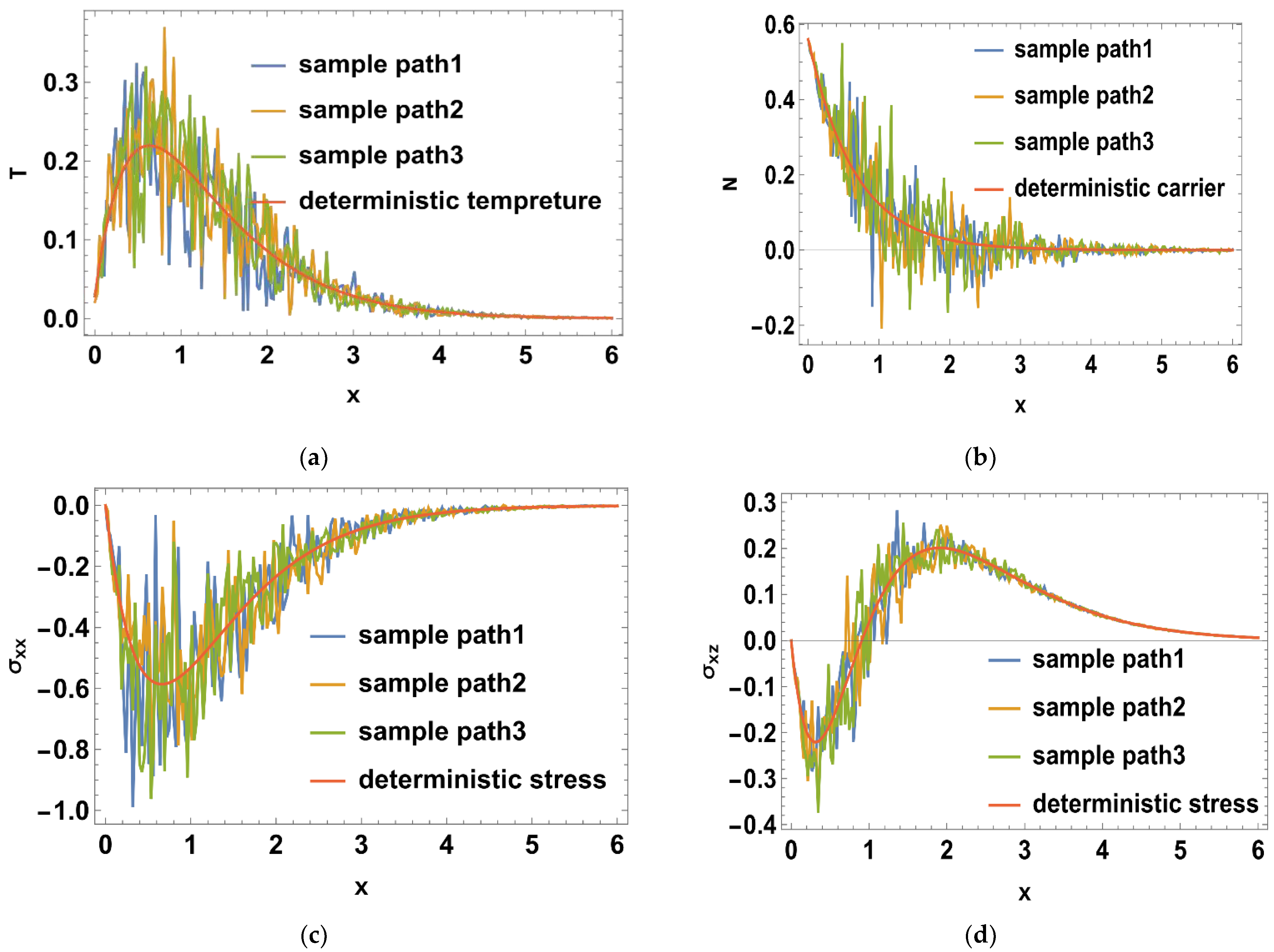
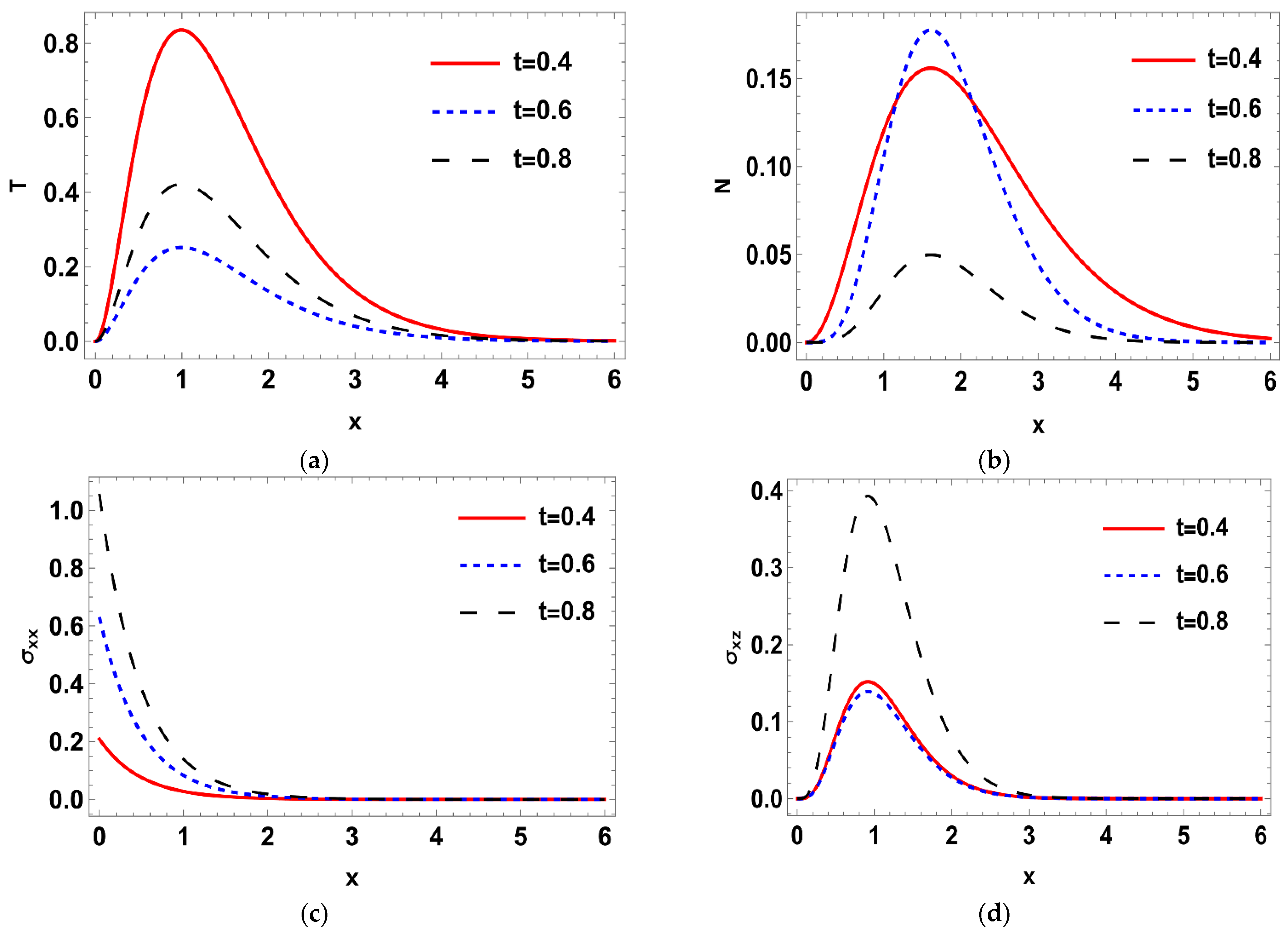
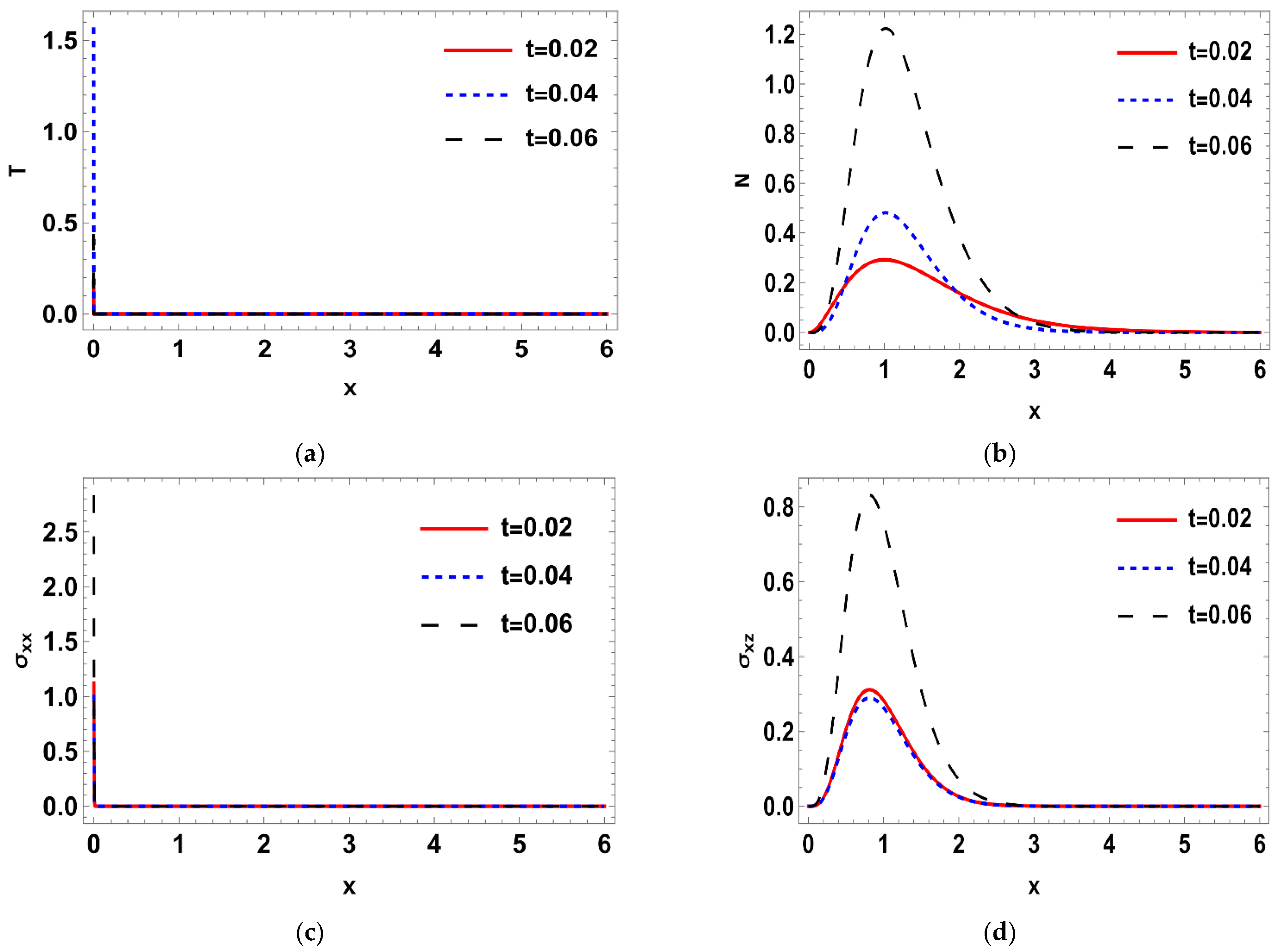
6.1. Stochastic Temperature (Thermal Wave)

Now, combining the random function on the boundary of temperature, we have as [36,37]:

$$T_0(t)=T_0(t)+{\phi }_0(t)$$

(78)

where $T_0(t)=\frac{T*}{h\left(t\right)}$, $T^{\ast }$ is a constant temperature or reference temperature, $h\left(t\right)$ is the function of the Heaviside unit, and ${\phi }_0(t)$ is a stochastic process, which satisfies:

$$E\left[{\phi }_0(t)\right]=0$$

(79)

Taking the stochastic process ${\phi }_0(t)$ of the white noise kind, each physical field now becomes a stochastic process as it contains the random function ${\phi }_0(t)$ on the boundary. Hence, from Equations (76), (78), and (79), we get:

$$E\left[T(x,t)\right]=T(x,t)$$

(80)

Since $E\left[{\phi }_0(t)\right]=0$, the mean of all the sample paths of the temperature field $E[T(x,t)]$ is the same as the solution for the deterministic case.

In this case, rewriting the temperature distribution as the following:

$$\begin{array}{cc}\hfill T(x,t)=& \theta (x,t)+\mathsf{\Theta }(x,t)T_0(t),or\hfill \\ \hfill T(x,t)=& \left(A_{11}+A_{12}{T}_0(t)\right)\exp (-k_{1}x+\omega t+Ibz)+\left(A_{13}+A_{14}{T}_0(t)\right)\exp (-k_{2}x+\omega t+Ibz)+\hfill \\ & \left(A_{15}+A_{16}{T}_0(t)\right)\exp (-k_{3}x+\omega t+Ibz)\hfill \end{array}\}$$

(81)

where the main coefficients are obtained in the Appendix A.

Such that $\theta (x,t)$ and $\mathsf{\Theta }(x,t)$, can be defined as:

$$\theta (x,t)=A_{11}\exp (-k_{1}x+\omega t+Ibz)+A_{13}\exp (-k_{2}x+\omega t+Ibz)+A_{15}\exp (-k_{3}x+\omega t+Ibz)$$

(82)

$$\mathsf{\Theta }(x,t)=A_{12}\exp (-k_{1}x+\omega t+Ibz)+A_{14}\exp (-k_{2}x+\omega t+Ibz)+A_{16}\exp (-k_{3}x+\omega t+Ibz)$$

(83)

With the help of Equations (78) and (81), $T\left(x,t\right)$ can be reduced to as [36,37]:

$$T(x,t)=\theta (x,t)+\mathsf{\Theta }(x,t)\left[T(t)+{\phi }_0(t)\right]$$

(84)

The above equation can be reduced to:

$$T(x,t)=\left\{\theta (x,t)+\mathsf{\Theta }(x,t)T(t)\right\}+\Phi (x,t){\phi }_0(t)$$

(85)

Reducing it to:

$$T(x,t)=T^1(x,t)+\mathsf{\Theta }(x,t){\phi }_0(t)$$

(86)

where $T^1(x,t)=\theta (x,t)+\mathsf{\Theta }(x,t)T_0(t)$.

By using the convolution property of the two functions $\mathsf{\Theta }\left(x,t\right)$ and ${\psi }_0(t)$

$$\left(f\ast g\right)\left(t\right)={\displaystyle {\int }_0^{t}f\left(\tau \right)}g\left(t-\tau \right)d\tau$$

(87)

we get:

$$T(x,t)=T^1(x,t)+{\displaystyle {\int }_0^t\mathsf{\Theta }(x,t-u)\phi (u)}du$$

(88)

where $T^1(x,t)$, is the distribution of deterministic temperature and $\mathsf{\Theta }(x,t-u)\phi (u)$ is the convolution function of Equation (88). Hence, Equation (88) can be reduced to:

$$T(x,t)=T^1(x,t)+{\displaystyle {\int }_0^t\mathsf{\Theta }(x,t-u)}dW\left(u\right)$$

(89)

where $W(u)$ expressed the Wiener process function. Squaring Equation (89), we get:

$$\begin{array}{cc}\hfill {\left[T(x,t)\right]}^2=& {\left[T^1(x,t)\right]}^2+{\displaystyle \underset{0}{\overset{t}{\int }}{\displaystyle \underset{0}{\overset{t}{\int }}\phi (u_1)\phi (u_2)d{u}_{1}d{u}_2\mathsf{\Theta }(x,t-u_1)\mathsf{\Theta }(x,t-u_2)}}+\hfill \\ & 2{\displaystyle \underset{0}{\overset{t}{\int }}{T}^1(x,t)\phi (u)\mathsf{\Theta }(x,t-u)du}\hfill \end{array}\}.$$

(90)

Taking the operator of expectation for both sides of the above equation, we get:

$$\begin{array}{cc}\hfill E{\left[T(x,t)\right]}^2=& E{\left[T^1(x,t)\right]}^2+{\displaystyle \underset{0}{\overset{t}{\int }}{\displaystyle \underset{0}{\overset{t}{\int }}E\left[\phi (u_1)\phi (u_2)\right]d{u}_{1}d{u}_2\mathsf{\Theta }(x,t-u_1)\mathsf{\Theta }(x,t-u_2)+}}\hfill \\ & 2{\displaystyle \underset{0}{\overset{t}{\int }}E\left[\phi (u)\right]T^1(x,t)\mathsf{\Theta }(x,t-u)du}\hfill \end{array}\}.$$

(91)

Recalling that:

$$E\left[\phi \left(u\right)\right]=0,E\left[\phi \left(u_1\right)\phi \left(u_2\right)\right]=\delta \left(u_1-u_2\right).$$

(92)

Then, Equation (91) is reduced to:

$$Var\left[T(x,t)\right]={\displaystyle \underset{0}{\overset{t}{\int }}{\displaystyle \underset{0}{\overset{t}{\int }}\mathsf{\Theta }\left(x,t-u_1\right)\mathsf{\Theta }\left(x,t-u_2\right)\delta \left(u_2-u_1\right)d{u}_{1}d{u}_2}}.$$

(93)

such that $Var\left[T(x,t)\right],$ is the variance of the temperature.

Recalling the property:

$${\displaystyle \underset{a}{\overset{b}{\int }}f\left(x\right)}f\left(x-x_0\right)dx=f\left(x_0\right),\hspace{1em}\hspace{1em}\hspace{1em}a<x_0<b.$$

(94)

The variance can be reduced as:

$$Var\left[T(x,t)\right]={\displaystyle \underset{0}{\overset{t}{\int }}\mathsf{\Theta }\left(x,t-u_1\right)\mathsf{\Theta }\left(x,t-u_2\right)d{u}_1}$$

(95)

Putting, $u_1=u_2$ yields:

$$Var\left[T(x,t)\right]={\displaystyle \underset{0}{\overset{t}{\int }}{\left[\mathsf{\Theta }\left(x,t-u_1\right)\right]}^{2}d{u}_1}.$$

(96)

Replacing $t-u_1$ by $\vartheta$, the variance of temperature can be defined as:

$$Var\left[T(x,t)\right]=-{\displaystyle \underset{t}{\overset{o}{\int }}{\left[\mathsf{\Theta }\left(x,\vartheta \right)\right]}^{2}d\vartheta }={\displaystyle \underset{0}{\overset{t}{\int }}{\left[\mathsf{\Theta }\left(x,\vartheta \right)\right]}^{2}d\vartheta }.$$

(97)

6.2. Deterministic Stress Distribution

By repeating the same method used in Section 6.1, but using the boundary condition of Equations (70) and (74), the deterministic solution of the stress can be rewritten as [36,37]:

$$\begin{array}{l}{\sigma }_{xx}(x,t)=H_{41}{D}_1\exp (-k_{1}x+\omega t+Ibz)+H_{42}{D}_2\exp (-k_{2}x+\omega t+Ibz)+H_{43}{D}_3\exp (-k_{3}x+\omega t+Ibz)+\\ H_{44}{D}_4\exp (-k_{4}x+\omega t+Ibz)\end{array}$$

(98)

6.3. Stochastic Stress Distribution

Using the Equation (78) and the condition of Equation (79), and proceeding described in Section 6.1, we get:

$$E\left[{\sigma }_{xx}(x,t)\right]={\sigma }_{xx}(x,t)$$

(99)

So, the mean of all the sample paths of the stress distribution $E\left[{\sigma }_{xx}(x,t)\right]$, equal to its deterministic case in Equation (98).

Then, Equation (98), can be rewritten as:

$$\begin{array}{cc}\hfill {\sigma }_{xx}(x,t)=& \mathsf{\Omega }(x,t)+\mathbb{S}(x,t)T_0,or\hfill \\ \hfill {\sigma }_{xx}(x,t)=& \left(E_{11}+E_{12}{T}_0(t)\right)\exp (-k_{1}x+\omega t+Ibz)+\left(E_{13}+E_{14}{T}_0(t)\right)\exp (-k_{2}x+\omega t+Ibz)+\hfill \\ & \left(E_{15}+E_{16}{T}_0(t)\right)\exp (-k_{3}x+\omega t+Ibz)+\left(E_{17}+E_{18}{T}_0(t)\right)\exp (-k_{4}x+\omega t+Ibz)\hfill \end{array}\}$$

(100)

such that $\mathsf{\Omega }(x,t)$ can be defined as:

$$\mathsf{\Omega }(x,t)=\begin{array}{l}{E}_{11}\exp (-k_{1}x+\omega t+Ibz)+E_{13}\exp (-k_{2}x+\omega t+Ibz)+\\ E_{15}\exp (-k_{3}x+\omega t+Ibz)+E_{17}\exp (-k_{4}x+\omega t+Ibz)\end{array}\}$$

(101)

and $\mathbb{S}(x,t)$, can be defined as:

$$\mathbb{S}(x,t)=\begin{array}{l}{E}_{12}\exp (-k_{1}x+\omega t+Ibz)+E_{14}\exp (-k_{2}x+\omega t+Ibz)+\\ E_{16}\exp (-k_{3}x+\omega t+Ibz)+E_{18}\exp (-k_{4}x+\omega t+Ibz)\end{array}\}$$

(102)

Using the stochastic boundary Equation (78), Equation (100) can be rearranged as:

$${\sigma }_{xx}(x,t)=\mathsf{\Omega }(x,t)+\mathbb{S}(x,t)\left[T_0+{\phi }_0(t)\right]$$

(103)

After reducing Equation (103), and using the convolution property, for the two functions $\mathbb{S}(x,t)$ and ${\psi }_0(t)$, we get:

$${\sigma }_{xx}(x,t)={\sigma }^1(x,t)+{\displaystyle {\int }_0^t\mathbb{S}(x,t-u)\phi (u)}du$$

(104)

where ${\sigma }^1\left(x,t\right)$ is the stress distribution. By the same method described in Section 6.1, we get the variance for the stress distribution as:

$$Var\left[{\sigma }_{xx}(x,t)\right]={\displaystyle \underset{0}{\overset{t}{\int }}{\mathbb{S}}^2(x,\vartheta )d\vartheta }$$

(105)

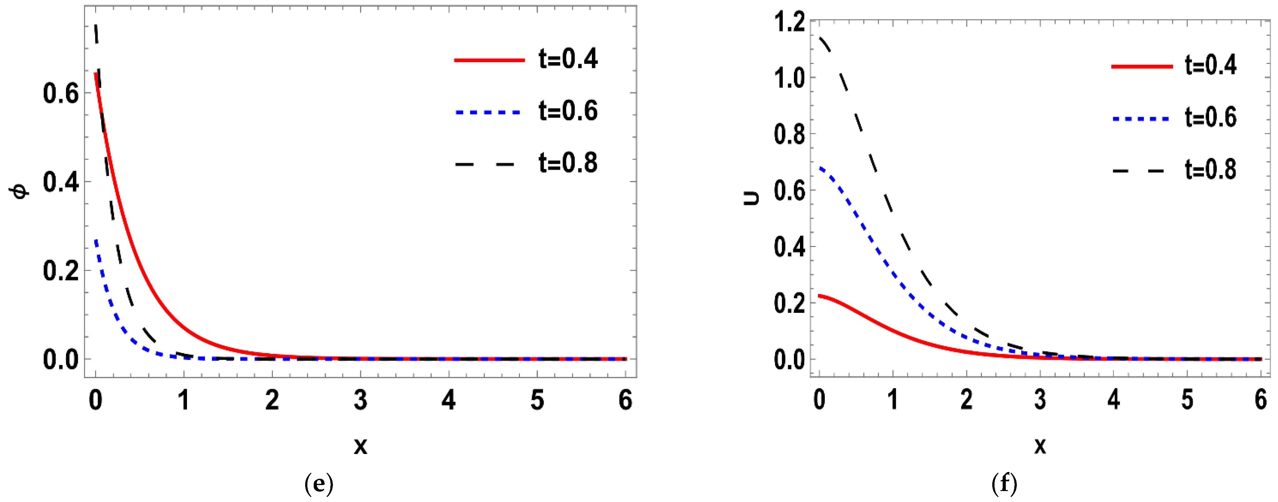
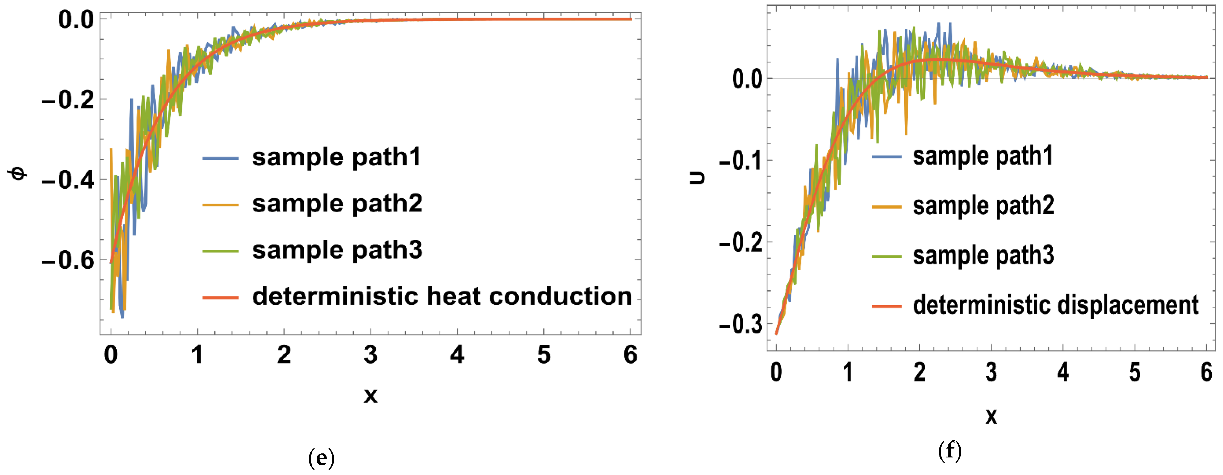
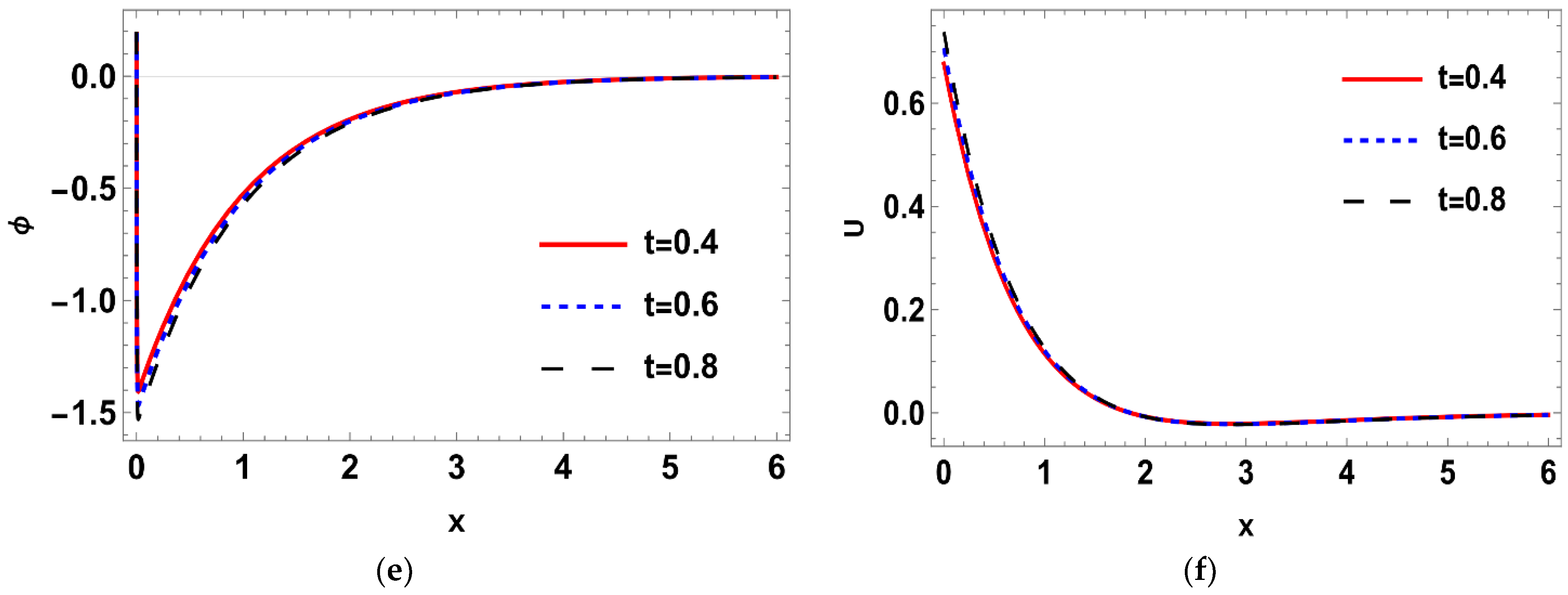
6.4. Deterministic Displacement Distribution

By repeating the same method used in Section 6.1, but using the boundary condition of Equations (65) and (66), the deterministic solution of the displacement can be rewritten as [36,37]:

$$\overline{u}(x,s)=\begin{array}{l}{H}_{21}{D}_1\exp (-k_{1}x+\omega t+Ibz)+H_{22}{D}_2\exp (-k_{2}x+\omega t+Ibz)+\\ H_{23}{D}_3\exp (-k_{3}x+\omega t+Ibz)+H_{24}{D}_4\exp (-k_{4}x+\omega t+Ibz)\end{array}\}$$

(106)

6.5. Stochastic Displacement Distribution

Using Equation (78) and the condition of Equation (79), and proceeding as described in Section 6.1, we get:

$$E\left[u(x,t)\right]=u(x,t)$$

(107)

Therefore, the mean of all the sample paths of the displacement distribution$E\left[u(x,t)\right]$ equals its deterministic case in Equation (106). Then, Equation (106) can be rewritten as:

$$\begin{array}{cc}\hfill u(x,t)=& \mathsf{\Gamma }\left(x,t\right)+U\left(x,t\right)T_0,or\hfill \\ \hfill u(x,t)=& \left(D_{11}+D_{12}{T}_0(t)\right)\exp (-k_{1}x+\omega t+Ibz)+\left(D_{13}+D_{14}{T}_0(t)\right)\exp (-k_{2}x+\omega t+Ibz)+\hfill \\ & \left(D_{15}+D_{16}{T}_0(t)\right)\exp (-k_{3}x+\omega t+Ibz)+\left(D_{17}+D_{18}{T}_0(t)\right)\exp (-k_{4}x+\omega t+Ibz)\hfill \end{array}\}$$

(108)

Such that $\mathsf{\Gamma }\left(x,t\right)$ can be defined as:

$$\mathsf{\Gamma }(x,t)=\begin{array}{l}{D}_{11}\exp (-k_{1}x+\omega t+Ibz)+D_{13}\exp (-k_{2}x+\omega t+Ibz)+\\ D_{13}\exp (-k_{3}x+\omega t+Ibz)+D_{14}\exp (-k_{4}x+\omega t+Ibz)\end{array}\}$$

(109)

On the other hand, $U\left(x,t\right)$ can be defined as:

$$U(x,t)=\begin{array}{l}{D}_{12}\exp (-k_{1}x+\omega t+Ibz)+D_{14}\exp (-k_{2}x+\omega t+Ibz)+\\ D_{16}\exp (-k_{3}x+\omega t+Ibz)+D_{18}\exp (-k_{4}x+\omega t+Ibz)\end{array}\}$$

(110)

Using the stochastic boundary Equation (78), Equation (108) can be rearranged as:

$$u(x,t)=\mathsf{\Gamma }\left(x,t\right)+U\left(x,t\right)\left[T\left(t\right)+{\phi }_0(t)\right]$$

(111)

Under the influence of the convolution property, Equation (111) can be reduced as:

$$u(x,t)=u^1(x,t)+{\displaystyle {\int }_0^{t}U(x,t-u)\phi (u)}du$$

(112)

where $u^1(x,t)$ is the deterministic displacement field.

By the same method described in Section 6.1, we get the variance for the displacement distribution as:

$$Var\left[u(x,t)\right]={\displaystyle \underset{0}{\overset{t}{\int }}{U}^2(x,\vartheta )d\vartheta }$$

(113)

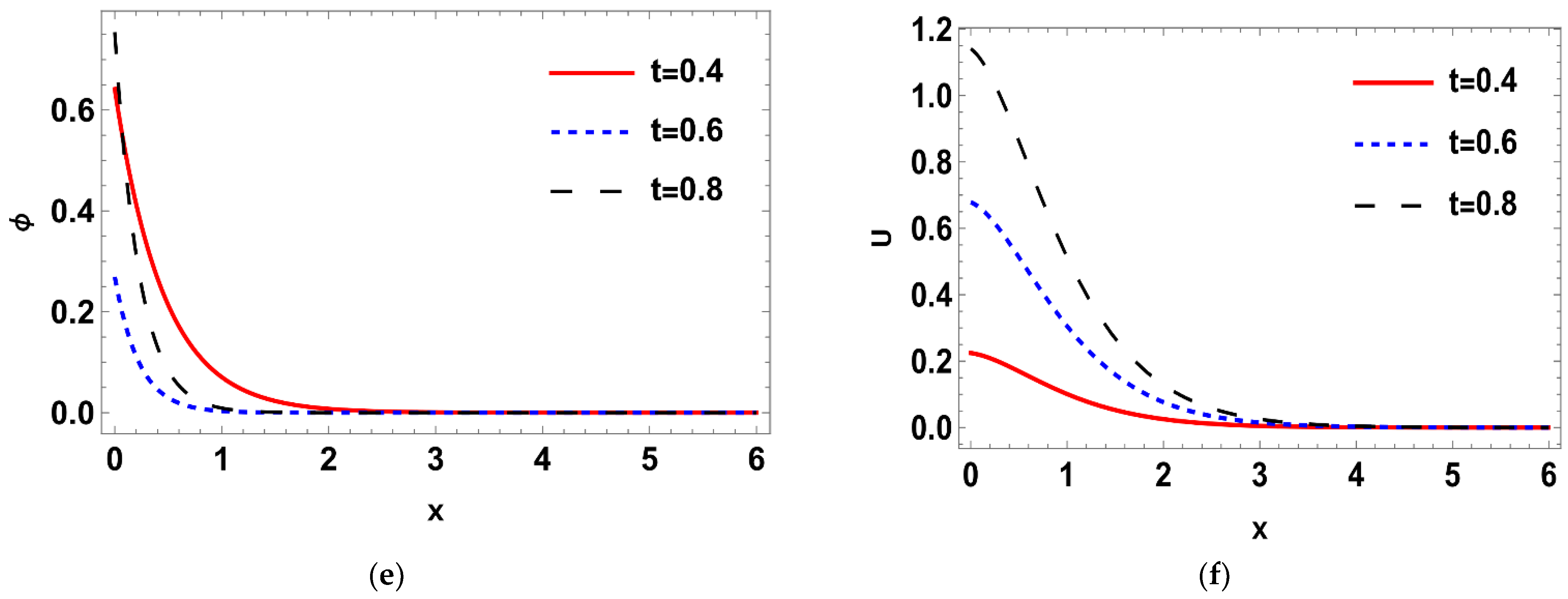
6.6. Deterministic Carrier Density Distribution

By repeating the same method used in Section 6.1, but using the boundary condition of Equations (73) and (77), we can rewrite the deterministic solution of the carrier density field as [36,37]:

$$N(x,t)=\begin{array}{l}{H}_{11}{D}_1\exp (-k_{1}x+\omega t+Ibz)+H_{12}{D}_2\exp (-k_{2}x+\omega t+Ibz)+\\ H_{13}{D}_3\exp (-k_{3}x+\omega t+Ibz)+H_{14}{D}_4\exp (-k_{4}x+\omega t+Ibz)\end{array}\}$$

(114)

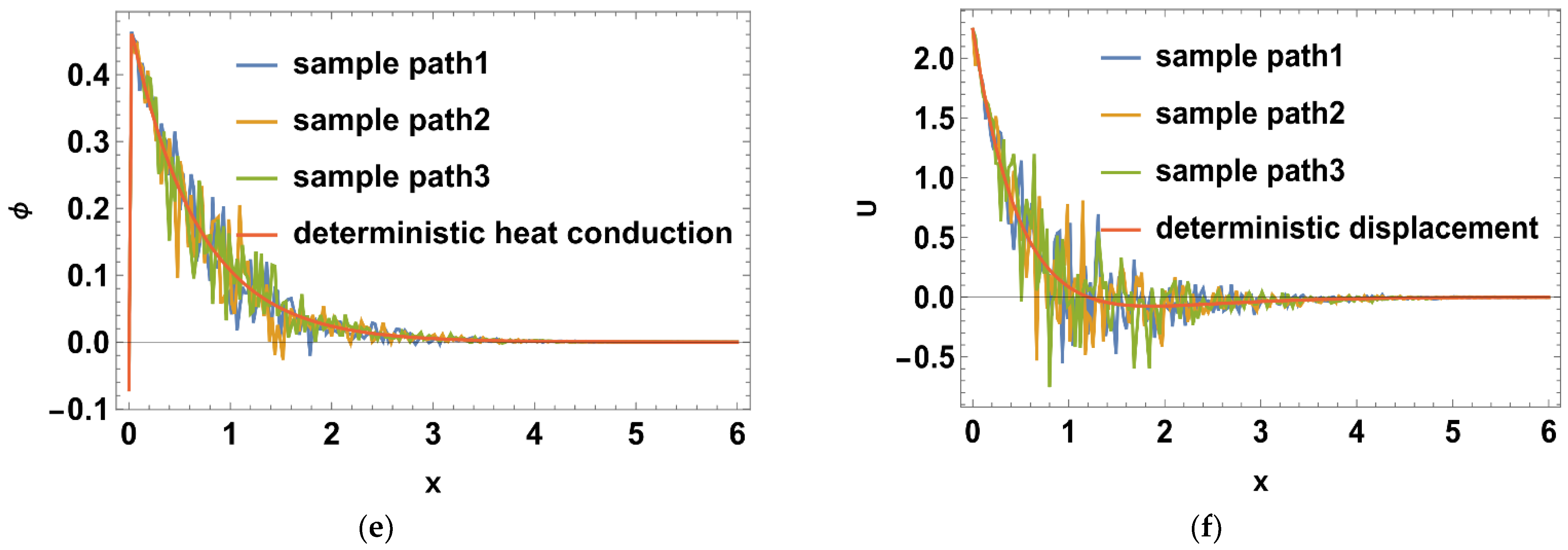
6.7. Stochastic Carrier Density Distribution

Using the Equation (78) and the condition of Equation (79), and proceeding as described in Section 6.1, we get:

$$E\left[N(x,t)\right]=N(x,t)$$

(115)

So, the mean of all the sample paths of the stress distribution $E\left[{\sigma }_{xx}(x,t)\right]$, equals its deterministic case in Equation (114). Then, Equation (114) can be rewritten as:

$$\begin{array}{cc}N(x,t)=& \omega \left(x,t\right)+\mathbb{Z}\left(x,t\right)T_0,or\hfill \\ \hfill N(x,t)=& \left(B_{11}+B_{11}{T}_0(t)\right)\exp (-k_{1}x+\omega t+Ibz)+\left(B_{13}+B_{14}{T}_0(t)\right)\exp (-k_{2}x+\omega t+Ibz)+\hfill \\ & \left(B_{15}+B_{16}{T}_0(t)\right)\exp (-k_{3}x+\omega t+Ibz)+\left(B_{17}+B_{18}{T}_0(t)\right)\exp (-k_{4}x+\omega t+Ibz)\hfill \end{array}\}$$

(116)

where the values of $\omega \left(x,t\right)$ and $\mathbb{Z}\left(x,t\right)$ take the form:

$$\omega (x,t)=\begin{array}{l}{B}_{11}\exp (-k_{1}x+\omega t+Ibz)+B_{13}\exp (-k_{2}x+\omega t+Ibz)+\\ B_{15}\exp (-k_{3}x+\omega t+Ibz)+B_{17}\exp (-k_{4}x+\omega t+Ibz)\end{array}\}$$

(117)

$$\mathbb{Z}(x,t)=\begin{array}{l}{B}_{12}\exp (-k_{1}x+\omega t+Ibz)+B_{14}\exp (-k_{2}x+\omega t+Ibz)+\\ B_{16}\exp (-k_{3}x+\omega t+Ibz)+B_{18}\exp (-k_{4}x+\omega t+Ibz)\end{array}\}$$

(118)

Using the stochastic boundary Equation (78), Equation (116) can be rearranged as:

$$N(x,t)=\omega \left(x,t\right)+\mathbb{Z}\left(x,t\right)\left[T_0\left(t\right)+{\phi }_0(t)\right]$$

(119)

Under the influence of the convolution property, Equation (119) can be reduced as:

$$N(x,t)=N^1(x,t)+{\displaystyle {\int }_0^t\mathbb{Z}(x,t-u)\phi (u)}du$$

(120)

where $N^1(x,t)$ is the deterministic carrier density field.

By the same method as described in Section 6.1, we get the variance for the carrier density field as:

$$Var\left[N(x,t)\right]={\displaystyle \underset{0}{\overset{t}{\int }}{\mathbb{Z}}^2(x,\vartheta )d\vartheta }$$

(121)

6.8. Deterministic Heat Conduction

By repeating the same method used in Section 6.1, but using the boundary condition of Equation (61), the deterministic solution of the heat conduction can be rewritten as [36,37]:

$$\overline{\varphi }(x,s)=\begin{array}{l}{H}_{31}{D}_1\exp (-k_{1}x+\omega t+Ibz)+H_{32}{D}_2\exp (-k_{2}x+\omega t+Ibz)+\\ H_{33}{D}_3\exp (-k_{3}x+\omega t+Ibz)+H_{34}{D}_4\exp (-k_{4}x+\omega t+Ibz)\end{array}\}$$

(122)

6.9. Stochastic Heat Conduction

Using the Equation (78) and the condition of Equation (79), and proceeding as described in Section 6.1, we get:

$$E\left[\varphi (x,t)\right]=\varphi (x,t)$$

(123)

So, the mean of all the sample paths of the heat conduction distribution, $E\left[\varphi (x,t)\right]$ equals its deterministic case in Equation (122). Then, Equation (122) can be rewritten as:

$$\begin{array}{cc}\hfill \varphi (x,t)=& H(x,t)+\mathsf{\Xi }(x,t)T_0,or\hfill \\ \hfill \varphi (x,t)=& \left(F_{11}+F_{12}{T}_0(t)\right)\exp (-k_{1}x+\omega t+Ibz)+\left(F_{13}+F_{14}{T}_0(t)\right)\exp (-k_{2}x+\omega t+Ibz)+\hfill \\ & \left(F_{15}+F_{16}{T}_0(t)\right)\exp (-k_{3}x+\omega t+Ibz)+\left(F_{17}+F_{18}{T}_0(t)\right)\exp (-k_{4}x+\omega t+Ibz)\hfill \end{array}\}$$

(124)

such that $H(x,t)$ can be defined as

$$H(x,t)=\begin{array}{l}{F}_{11}\exp (-k_{1}x+\omega t+Ibz)+F_{13}\exp (-k_{2}x+\omega t+Ibz)+\\ F_{15}\exp (-k_{3}x+\omega t+Ibz)+F_{17}\exp (-k_{4}x+\omega t+Ibz)\end{array}\}$$

(125)

and $\mathsf{\Xi }(x,t)$ can be defined as:

$$\mathbb{S}(x,t)=\begin{array}{l}{F}_{12}\exp (-k_{1}x+\omega t+Ibz)+F_{14}\exp (-k_{2}x+\omega t+Ibz)+\\ F_{16}\exp (-k_{3}x+\omega t+Ibz)+F_{18}\exp (-k_{4}x+\omega t+Ibz)\end{array}\}$$

(126)

Using the stochastic boundary Equation (78), then Equation (124), can be rearranged as:

$$\varphi (x,t)=H(x,t)+\mathsf{\Xi }(x,t)\left[T_0+{\phi }_0(t)\right]$$

(127)

After reducing Equation (127), and using the convolution property again for the two functions $\mathsf{\Xi }(x,t)$ and ${\psi }_0(t)$, we get:

$$\varphi (x,t)={\varphi }^1(x,t)+{\displaystyle {\int }_0^t\mathsf{\Xi }(x,t-u)\phi (u)}du$$

(128)

where ${\varphi }^1(x,t)$ is the heat conduction distribution. By the same method as described in Section 6.1, the variance for heat conduction distribution can be obtained as:

$$Var\left[\varphi (x,t)\right]={\displaystyle \underset{0}{\overset{t}{\int }}{\mathsf{\Xi }}^2(x,\vartheta )d\vartheta }$$

(129)

7. Numerical Results and Discussions

The Silicon (Si) material was chosen as a semiconductor example of our problem to carry out the numerical simulations. The parameters of Si are given in SI units below in

Table 1. The physical constants of Si medium.

$\lambda =3.64\times {10}^{10}\mathrm{N}/{\mathrm{m}}^2$	$\mu =5.46\times {10}^{10}\mathrm{N}/{\mathrm{m}}^2$	$\rho =2330\mathrm{kg}/{\mathrm{m}}^3$	$\tau =5\times {10}^{-5}\mathrm{s}$
$T_0=800\mathrm{K}$	$d_n=-9\times {10}^{-31}{\mathrm{m}}^3$	$D_E=2.5\times {10}^{-3}{\mathrm{m}}^2/\mathrm{s}$	$E_g=1.11\mathrm{eV}$
$C_e=695\mathrm{J}/(\mathrm{kg}\mathrm{K})$	${\alpha }_t=4.14\times {10}^{-6}{\mathrm{K}}^{-1}$	$s=2\mathrm{m}/\mathrm{s}$	$t=0.8$
${\omega }_0=-0.3$	$z=1$	$\xi =0.1$	$b=1$
${\epsilon }_0=8.85\times {10}^{-12}\mathrm{F}/\mathrm{m}$	$p_1=2$	${\mu }_0=4\pi \times {10}^{-7}\mathrm{H}/\mathrm{m}$

as [42,43]:

Such that $\omega ={\omega }_0+i\xi ,$ where $i$ is the imaginary part, $e^{\omega t}=e^{{\omega }_{0}t}(\cos \xi t+i\sin \xi t)$ and for a short time, the real part, $\omega ={\omega }_0$ was taken. The calculations were performed for three values of time, namely: $t=0.4$, $t=0.6$, and $t=0.8$ Normal mode method was used to get the solutions of the distribution of the thermal temperature $\theta$, Carrier density N, the stress (${\sigma }_{xx},{\sigma }_{xz}$) distribution, heat conduction $\phi$, and the displacement components $u$. The problem was described in 2-D and in non-dimensional form. Figure 1a–d shows the difference in the deterministic case of the physical quantities in three different times namely, at $t=0.4,t=0.6\mathrm{and}t=0.8$ when $a=5$. It is notable that the wave of all physical quantities behaves in the same manner but differ a bit in the magnitude. In Figure 1a, the deterministic distribution of the temperature begins from a lowest point then becomes greater towards the maximum, then becomes less smooth as x-axis increases until it matches the zero line. In Figure 1b, the deterministic carrier density distribution starts from the peak, then goes down till it matches the zero line. In Figure 1c,d, it is noted that the stress distributions (${\sigma }_{xx},{\sigma }_{xz}$) agree with the boundary conditions which start from zero, then decrease a little after a short distance, then begin to raise again until coincide with zero line. In Figure 1e,f, it is noted that the heat conduction $\phi$ and the displacement components $u$ take the same distribution as a wave, but differ in terms of amplitude. The displacement component $u$ still goes up to the positive part, but the heat conduction $\phi$ remains at the negative part. Figure 2a–f. shows the disparity between the deterministic and stochastic distributions of temperature, normal stress, carrier density, displacement, and heat conduction distributions versus x-axis at $t=0.4$ when $a=5$. It is noted that, in all distributions, the intensity of the white noise looks very strong at first, then begins to get weak with the increasing of the distance. Finally, it coincides with x-axis. These findings (the deterministic results) are consistent with what has been shown in real-world experiments [44,45]. Figure 3a–f, display the variance of temperature, normal stress, carrier density, displacement, and heat conduction distributions around its mean at different values of times, namely $t=0.4,t=0.6\mathrm{and}t=0.8.$ when $a=5$. Figure 3, especially Figure 3a,b,d, represents the variance of the thermal wave of temperature$\theta$, carrier density $N$ and the stress ${\sigma }_{xz}$ distributions, respectively. It is noted that they act similarly as they begin from zero, and then take pyramidal shape as a wave but in a different size, then decrease to coincide with the zero line. Figure 3c,e,f, represent the variance of the stress ${\sigma }_{xx}$, heat conduction, and displacement distributions respectively. They also take the same behavior as they begin from the peak and then decrease smoothly till match the x-axis. Figure 4a–f, shows the deterministic temperature, normal stress, carrier density, displacement, and heat conduction distributions along the distance for various values of times, namely $t=0.4,t=0.6andt=0.8.$ when $a=0$. It is noted that all distributions match the boundary condition, as they begin from a maximum or minimum point, then decrease or increase in a smooth way, except the stress ${\sigma }_{xz}$ and heat conduction $\phi$ distributions; as they decrease sharply not smoothly, then coincide with x-axis. Figure 5a–f, display the deterministic and stochastic distributions of temperature $T$, normal stress ${\sigma }_{xx}$, carrier density $N$, displacement $u$ and heat conduction $\phi$ distributions along the distance at $t=0.4$ when $a=0$. It is noted that they agree with the boundary condition and the strength of the random function begins very strong, then weakens with the increasing of x-axis until it vanishes. Figure 6a–f, shows the variance of temperature $T$, normal stress ${\sigma }_{xx}$, carrier density $N$, displacement $u$ and heat conduction $\phi$ distributions around its mean at different values of times $t=0.4,t=0.6andt=0.8.$ when $a=0$. Figure 6a,c,e represent (the temperature $T$, normal stress ${\sigma }_{xx}$ and heat conduction $\phi$ distributions), respectively. It is noted that it takes the same shape as a wave, beginning from the peak, then dropping sharply to the lowest point and coinciding with x-axis. Figure 7a–f shows the effect of the two-temperature parameter {a}. In order to show the effect of two-temperature parameter {a}, a comparison between the temperature $T$, carrier density N, stress ${\sigma }_{xx}$and ${\sigma }_{xz}$, heat conduction $\phi ,$ and displacement distributions was performed in two different values of two-temperature parameter, namely $a=0$ and $a=5$. It is noted that, when $a=0.0$, the curves of temperature $T$, carrier density $N$, and displacement distributions begin from a maximum point, then decrease smoothly till coincide with x-axis. On the other side the curves of stress, ${\sigma }_{xx}$ and ${\sigma }_{xz}$, heat conduction $\phi$ begins from a maximum point, then decreases sharply, then increases again smoothly till coinciding with the zero line. It is noted that, when $a=5$, the curves of the temperature $T$, the stress (${\sigma }_{xx}$, ${\sigma }_{xz}$) and displacement distribution $u$ begin from a minimum point then increase smoothly till coinciding with x-axis, but the carrier density N and the heat conduction $\phi$ distributions begin from a maximum point, then decrease smoothly till coinciding with x-axis. From Figure 7a–f, it is noted that the increase of the two-temperature parameter leads to the increase of its magnitude for all physical quantities, except for the displacement distribution. Taking into account the increase in the time of deterministic behavior is more realistic than the stochastic behavior, and physically acceptable as well as consistent with the experimental results implemented by Xiao et al. [44]. The thermal wave (temperature) and plasma wave (carrier density) behavior are compatible with those of the experiments specified in the subfigures of temperature and carrier density distribution [45].

8. Conclusions

The basic idea of this research relies on two different types of analyses: deterministic and stochastic types. The utilized stochastic type is determined when the Gaussian white noise function is combined with the boundary condition. The random function was used because of the nature of the problem, i.e., its distribution is different at different times. Using the normal mod method, the numerical solutions of deterministic and stochastic for temperature, stress, carrier density, heat conduction, and displacement distributions were obtained. Because of the nature of the stochastic process, especially, the Wiener process, the statistical properties of the problem< such as the mean and variance, were calculated numerically. Mathematically, the variance was proven as a function of the square of the noise amplitude. Graphically, it was found that the paths of the variance solutions propagate to zero as the distance increases. It is noticed how the two-temperature parameter affects greatly the distributions of temperature, heat conduction, displacement components, and normal stress. However, there are no notable effects on the carrier density distribution. All distributions of deterministic and stochastic go to zero as x-axis increases to infinity. It was found that the two-temperature parameter has a great effect on the wave distribution, and it was found that it is more accurate than the one-temperature theory of generalized thermo-elasticity. Scientists and engineers can use the obtained results in developing some related models. When comparing the solutions, it can be concluded that the stochastic behavior is an important phenomenon and has a great influence on the distribution of different physical domains. This investigation may be very useful for scientists in the development of quality semiconductor fabrication and its physical and engineering applications. Many modern industries dependent on the gradient of temperature and stochastic behavior of semiconductors use electric circuits for various purposes in aircraft.

References

1. Biot, M.A. Thermoclasticity and irreversible thermodynamics. J. Appl. Phys. 1956, 27, 240–253. [Google Scholar] [CrossRef]
2. Lord, H.W.; Shulman, Y. A generalized dynamical theory of thermoelasticity. J. Mech. Phys. Solids 1967, 15, 299–309. [Google Scholar] [CrossRef]
3. Green, A.E.; Lindsay, K.A. Thermoelasticity. J. Elast. 1972, 2, 1–7. [Google Scholar] [CrossRef]
4. Chandrasekharaiah, D.S. Thermoelasticity with second sound: A review. Appl. Mech. Rev. 1986, 39, 355–376. [Google Scholar] [CrossRef]
5. Chandrasekharaiah, D.S. Hyperbolic thermoelasicity: A review of recent literature. Appl. Mech. Rev. 1998, 51, 705–729. [Google Scholar] [CrossRef]
6. Sharma, J.N.; Kumar, V.; Chand, D. Reflection of generalized thermoelastic waves from the boundary of a half-space. J. Therm. Stress. 2003, 26, 925–942. [Google Scholar] [CrossRef]
7. Fahmy, M.A. Boundary element modeling of 3 T nonlinear transient magneto-thermoviscoelastic wave propagation problems in anisotropic circular cylindrical shells. Compos. Struct. 2021, 277, 114655. [Google Scholar] [CrossRef]
8. Fahmy, M.A.; Almehmadi, M.M.; Al Subhi, F.M.; Sohail, A. Fractional boundary element solution of three-temperature thermoelectric problems. Sci. Rep. 2022, 12, 6760. [Google Scholar] [CrossRef]
9. Fahmy, M.A. 3D Boundary Element Model for Ultrasonic Wave Propagation Fractional Order Boundary Value Problems of Functionally Graded Anisotropic Fiber-Reinforced Plates, Fractal and Fractional. Fractal Fract. 2022, 6, 247. [Google Scholar] [CrossRef]
10. Fahmy, M.A.; Alsulami, M.O. Boundary Element and Sensitivity Analysis of Anisotropic Thermoelastic Metal and Alloy Discs with Holes. Materials 2022, 15, 1828. [Google Scholar] [CrossRef]
11. Fahmy, M.A. Boundary element modeling of fractional nonlinear generalized photothermal stress wave propagation problems in FG anisotropic smart semiconductors. Eng. Anal. Bound. Elem. 2022, 134, 665–679. [Google Scholar] [CrossRef]
12. Scutaru, M.L.; Vlase, S.; Marin, M.; Modrea, A. New analytical method based on dynamic response of planar mechanical elastic systems. Bound. Value Probl. 2020, 2020, 104. [Google Scholar] [CrossRef]
13. Zhang, L.; Bhatti, M.M.; Michaelides, E.E.; Marin, M.; Ellahi, R. Hybrid nanofluid flow towards an elastic surface with tantalum and nickel nanoparticles, under the influence of an induced magnetic field. Eur. Phys. J. Spec. Top. 2022, 231, 521–533. [Google Scholar] [CrossRef]
14. Abouelregal, A.E.; Marin, M. The response of nanobeams with temperature-dependent properties using state-space method via modified couple stress theory. Symmetry 2020, 12, 1276. [Google Scholar] [CrossRef]
15. Marin, M.; Ellahi, R.; Vlase, S.; Bhatti, M.M. On the decay of exponential type for the solutions in a dipolar elastic body. J. Taibah Univ. Sci. 2020, 14, 534–540. [Google Scholar] [CrossRef] [Green Version]
16. Gordon, J.P.; Leite, R.C.C.; Moore, R.S.; Porto, S.P.S.; Whinnery, J.R. Long-transient effects in lasers with inserted liquid samples. J. Appl. Phys. 1965, 36, 3–8. [Google Scholar] [CrossRef]
17. Kreuzer, L.B. Ultralow gas concentration infrared absorption spectroscopy. J. Appl. Phys. 1971, 42, 2934. [Google Scholar] [CrossRef]
18. Tam, A.C. Ultrasensitive Laser Spectroscopy; Kliger, D.S., Ed.; Academic Press: Cambridge, MA, USA, 1983; pp. 1–108. [Google Scholar]
19. Tam, A.C. Applications of photoacoustic sensing techniques. Rev. Mod. Phys. 1986, 58, 381. [Google Scholar] [CrossRef]
20. Tam, A.C. Photothermal Investigations in Solids and Fluids; Sell, J.A., Ed.; Academic Press: Cambridge, MA, USA, 1989; pp. 1–33. [Google Scholar]
21. Chen, P.J.; Gurtin, M.E.; Williams, W.O. On the thermodynamics of non-simple elastic materials with two temperatures. ZAMP 1969, 20, 107–112. [Google Scholar] [CrossRef]
22. Chen, J.K.; Beraun, J.E.; Tham, C.L. Ultrafast thermoelasticity for short-pulse laser heating. Int. J. Eng. Sci. 2004, 42, 793–807. [Google Scholar] [CrossRef]
23. Qiu, T.Q.; Tien, C.L. Heat transfer mechanism during short-pulse laser heating of metals. ASME J. Heat Transf. 1993, 115, 835–841. [Google Scholar] [CrossRef]
24. Youssef, H.M. Theory of two-temperature-generalized thermoelasticity. IMA J. Appl. Math. 2006, 71, 383–390. [Google Scholar] [CrossRef]
25. Lotfy, K. Two temperature generalized magneto-thermoelastic interactions in an elastic medium under three theories. Appl. Math. Comput. 2014, 227, 871–888. [Google Scholar] [CrossRef] [Green Version]
26. Lotfy, K.; Hassan, W. Normal mode method for two-temperature generalized thermoelasticity under thermal shock problem. J. Therm. Stress. 2014, 37, 545–560. [Google Scholar] [CrossRef]
27. Hoel, P.G.; Port, S.C.; Stone, C.J. Introduction to Stochastic Processes; Waveland Press: Long Grove, IL, USA, 1986. [Google Scholar]
28. Platen, E.; Kloeden, P. Numerical Solution of Stochastic Differential Equations; CRC Press: Boca Raton, FL, USA, 2006. [Google Scholar]
29. Lawler, G.F. Introduction to Stochastic Processes; CRC Press: Boca Raton, FL, USA, 2006. [Google Scholar]
30. Hoel, P.G.; Port, S.C.; Stone, C.J. Introduction to Stochastic Processes; Universal Book Stall: New Delhi, India, 1972. [Google Scholar]
31. Sherief, H.H.; El-Maghraby, N.M.; Allam, A.A. Stochastic thermal shock problem in generalized thermoelasticity. Appl. Math. Model. 2013, 37, 762–775. [Google Scholar] [CrossRef]
32. Sherief, H.H.; El-Maghraby, N.M.; Allam, A.A. Stochastic thermal shock problem and study of wave propagation in the theory of generalized thermoelastic diffusion. Math. Mech. Solids 2016, 22, 1767–1789. [Google Scholar] [CrossRef]
33. Kloeden, P.E.; Platen, E. Numerical Solution of Stochastic Differential Equations; Applications of Mathematics Series; Springer: Berlin/Heidelberg, Germany, 1992; Volume 23. [Google Scholar]
34. Lotfy, K.; Ahmed, A.; El-Bary, A.; Tantawi, R.S. A Novel Stochastic Model of the Photo-Thermoelasticity Theory of the Non-Local Excited Semiconductor Medium. Silicon 2022. [Google Scholar] [CrossRef]
35. Bellomo, N.; Flandoli, F. Stochastic partial differential equations in continuum physics—On the foundations of the stochastic interpolation method for ITO’s type equations. Math. Comput. Simul. 1989, 31, 3–17. [Google Scholar] [CrossRef]
36. Kant, S.; Mukhopadhyay, S. Investigation of a problem of an elastic half space subjected to stochastic temperature distribution at the boundary. Appl. Math. Model. 2017, 46, 492–518. [Google Scholar] [CrossRef]
37. Val’kovskaya, V.I.; Lenyuk, M.P. Stochastic nonstationary temperature fields in a solid circular–cylindrical two-layer plate. J. Math. Sci. 1996, 79, 1483–1487. [Google Scholar] [CrossRef]
38. Todorović, D.M. Plasma, thermal, and elastic waves in semiconductors. Rev. Sci. Instrum. 2003, 74, 582–585. [Google Scholar] [CrossRef]
39. Vasilev, A.N.; Sandomirskii, V.B. Photoacoustic effects in finite semiconductors. Sov. Phys. Semicond. 1984, 18, 1095. [Google Scholar]
40. Christofides, C.; Othonos, A.; Loizidou, E. Influence of temperature and modulation frequency on the thermal activation coupling term in laser photothermal theory. J. Appl. Phys. 2002, 92, 1280. [Google Scholar] [CrossRef]
41. Song, Y.Q.; Bai, J.T.; Ren, Z.Y. Study on the reflection of photothermal waves in a semiconducting medium under generalized thermoelastic theory. Acta Mech. 2012, 223, 1545–1557. [Google Scholar] [CrossRef]
42. Lotfy, K.; Hassan, W.; Gabr, M.E. Thermomagnetic effect with two temperature theory for photothermal process under hydrostatic initial stress. Results Phys. 2017, 7, 3918–3927. [Google Scholar] [CrossRef]
43. Hobiny, A.D.; Abbas, I.A. A study on photothermal waves in an unbounded semiconductor medium with cylindrical cavity. Mech. Time-Depend. Mater. 2016, 21, 61–72. [Google Scholar] [CrossRef]
44. Xiao, Y.; Shen, C.; Zhang, W. Screening and prediction of metal-doped α-borophene monolayer for nitric oxide elimination. Mater. Today Chem. 2022, 25, 100958. [Google Scholar] [CrossRef]
45. Liu, J.; Han, M.; Wang, R.; Xu, S.; Wang, X. Photothermal phenomenon: Extended ideas for thermophysical properties characterization. J. Appl. Phys. 2022, 131, 065107. [Google Scholar] [CrossRef]
Figure 1. (af) The deterministic temperature, normal stress, carrier density, displacement and heat conduction distributions along the distance for various values of times in relation to generalized photothermoelasticity theory when a = 5 .
Crystals 13 00082 g001aCrystals 13 00082 g001b
Figure 2. (af) The deterministic and stochastic distributions of temperature, normal stress, carrier density, displacement and heat conduction distributions along the distance at t = 0.4 in relation to generalized photo-thermoelasticity theory, when a = 5 .
Crystals 13 00082 g002aCrystals 13 00082 g002b
Figure 3. (af) The variance of temperature, normal stress, carrier density, displacement and heat conduction distributions around its mean at different values of times t = 0.2, t = 0.4 and t = 0.6 when a = 5 .
Crystals 13 00082 g003aCrystals 13 00082 g003b
Figure 4. (af) The deterministic temperature, normal stress, carrier density, displacement and heat conduction distributions along the distance for various values of times in relation to generalized photo-thermoelasticity theory. when a = 0 .
Crystals 13 00082 g004aCrystals 13 00082 g004b
Figure 5. (af) The deterministic and stochastic distributions of temperature, normal stress, carrier density, displacement and heat conduction distributions along the distance at t = 0.4 in relation to generalized photo-thermoelasticity theory, when a = 0 .
Crystals 13 00082 g005aCrystals 13 00082 g005b
Figure 6. (af) The variance of temperature, normal stress, carrier density, displacement and heat conduction distributions around its mean at different values of times t = 0.2 , t = 0.4 and t = 0.6 , when a = 0 .
Crystals 13 00082 g006aCrystals 13 00082 g006b
Figure 7. (af) A comparison between deterministic cases at different values of two temperature parameter, namely; a = 0 and a = 5 when t = 0.4 .
Crystals 13 00082 g007aCrystals 13 00082 g007b