Appendix A. Numerical Calculation of the Spinodal Limit
When
, Equation (
9) for
no longer has a steady-state first integral. That means that
deviates from the simple form given in Equation (
17) and must be calculated numerically. The procedure is as follows: first, we set
and we then expand
F to second order in
. We note that the electric potential also must be expanded up to order 2 in
for this expansion to be correct, especially when calculating the tricritical point as in the next appendix. This can be done using Equation (
11), which gives (This expansion was not performed in an earlier work by Ribière et al. [
11] whose calculations, therefore, are not entirely correct, even in the simple case where
.):
After a straightforward calculation, we find that the total free energy can be written as
, where each term has the following form:
Minimizing the
term with respect to
leads in steady state to the following Euler–Lagrange equation for
:
This equation must be solved with the two BCs
.
We solved this equation with Mathematica 12 by using a shooting method with starting initial conditions: and , where is an arbitrary constant. Depending on the value of , we found two solutions corresponding to (sol 1) and (sol 2) in the final (steady) state. For each of these solutions, we then calculated and noted that, whatever the thickness, the value of found for sol 2 was always greater than that found for sol 1. This means that, at the spinodal limit, the -director of the TIC -or more simply the TIC– orients parallel to the magnetic field.
On
Figure A1, we compare the numerically calculated sol 1 with the approximate profile using Equation (
17) with
. As visible, these profiles are extremely close, which further validate the theoretical approach in the main text. Finally, the critical voltage
was determined numerically by finding for what value of
V the coefficient
calculated with sol 1 vanishes, leading to the following integral formula:
with
,
, and
. Evaluating this formula with the numerically calculated sol 1 gave the dashed red line of
Figure 2, which is also very close to the approximate formula given in the main text.
Figure A1.
Comparison between the exact profile
(solid line) obtained by solving Equation (
A6) with
T and the analytical profile (dashed line) found at
when
[Equation (
17)]. The sample thickness is
m and the cholesteric pitch is
m.
Figure A1.
Comparison between the exact profile
(solid line) obtained by solving Equation (
A6) with
T and the analytical profile (dashed line) found at
when
[Equation (
17)]. The sample thickness is
m and the cholesteric pitch is
m.
Appendix B. Order of the Transition between TIC and Homeotropic Structures (θ = 0)
Previous studies in the absence of magnetic field indicate the presence of a tricritical point on the spinodal line of coordinates with . At this point, the transition changes order, being second order when and first order when .
To find the position of the tricritical point in the presence of a magnetic field, a calculation to order 4 in a disturbance is necessary. This calculation is complicated because it is necessary to take into account not only the disturbance of the type
for angle
but also a disturbance of the type
for the angle
, as the previous appendix suggests when
(see Equation (
A6) and
Figure A1). Moreover, at order 4 in the disturbance, the electric field must be expanded at order 2 in
similar to the previous appendix.
As an approximation, we can neglect the disturbance in
, which leads to the following equation in
that must be solved to find the cell thickness at the tricritical point,
:
with
,
,
,
and:
Solving Equation (
A8) with the values of the material constants given in
Table 1 gives
m.
To test the accuracy of this prediction, we calculated the position of the tricritical point by solving numerically for each thickness Equations (
8)–(
10) in a small interval of voltages around
. In the following, we will set
and
, with
V (resp.,
) the final (resp., initial) voltage in our simulations as described above. In our calculations, we took
s
m
,
s,
,
and
large enough for the stationary regime to be reached. For the initial voltage, we took either
or
Vrms (
Vrms). In the first case, the initial state is the HN, while in the second, the system transits through a high amplitude TIC before relaxing towards the steady state. In the following, all the curves calculated by taking
will be drawn in blue, while those obtained by using
V will be drawn in red.
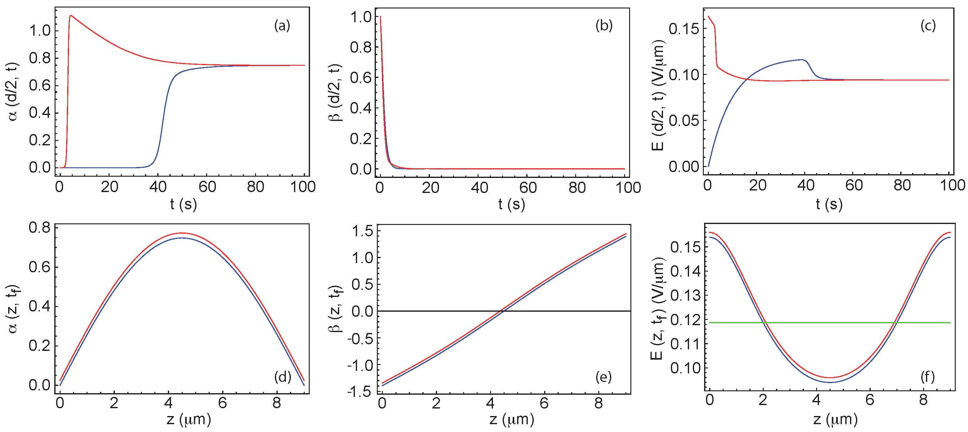
A first set of curves calculated this way is shown in
Figure A2 when
m and
Vrms. In this example,
and
for all cases. This shows that there is only one steady state here, corresponding to a TIC of finite amplitude oriented parallel to
B.
The situation is different at larger thickness as shown in
Figure A3 calculated by taking
m and
Vrms. In this particular example, two distinct stationary states are reached depending on the value of
: a TIC of small amplitude when
is small (here equal to 0) and a TIC with a larger amplitude when
is large enough (here equal to 0.5 Vrms). Note that these two TIC orient parallel to
B since
in the two cases (whatever the chosen value of
). The calculation of
F gives
for the TIC of small amplitude (blue curve) and
for the TIC of large amplitude. Here the energy is given in pN/
m. As a consequence, the TIC of small amplitude is metastable while the one of larger amplitude is stable. This calculation shows the existence of a first order transition line between two TIC parallel to
B with different amplitudes, in the vicinity of the spinodal line of the HN.
Figure A2.
Numerical solutions of Equations (
8)–(
10) at
m and
Vrms calculated by taking
(blue curves) and
Vrms (red curves). (
a–
c) Time evolution of the angles
and
and of the electric field
E in the middle of the sample; (
d–
f)
z-profiles of angles
and
and of the electric field
E in steady state. In graphs (
d–
f), the red curves have been shifted slightly upwards to become visible. In (
f) the green line shows the average electric field
.
Figure A3.
Numerical solutions at m and Vrms calculated by taking (blue curves) and (red curves). (a–c) Time evolution of the angles and and of the electric field E in the middle of the sample; (d–f) z-profiles of angles and and of the electric field E in steady state. In (f) the green line shows the average electric field . In this example, two different stationary solution are found. The blue one is stable, and the red one metastable.
To confirm this point and determine the order of the HN→TIC transition, we systematically calculated
as a function of
V at different thicknesses (
Figure A4). As before the blue curves were calculated by taking
Vrms and the red curves by taking
Vrms. With these values, we found that, in all cases, the TIC orients parallel to
B in the stationary regime (
). However, important changes appear depending on the thickness. At small thicknesses, the red and blue curves
are identical. They vary continuously at the transition, with a concave shape at all voltages
. This is characteristic of a second-order phase transition. An example calculated at
m is shown in
Figure A4a. At larger thicknesses, the situation becomes more complex. At
m, the red and blue curves are still identical and the HN→TIC transition is still second order, but we can note now that the curves deform above
and become convex at some intermediate voltages as can be seen in
Figure A4b.
Figure A4.
Amplitude of the TIC as a function of the voltage difference calculated at different thicknesses: m (a); m (b); m (c); m (d); m (e) and m (f). In (d–f), the dotted-dashed line indicates the value of at which the two solutions have the same energy. On the left (resp., right) of this line, the most stable solution is that of low (resp., large) amplitude.
The situation drastically changes at
m. At this thickness, the red and blue curves are different. The HN→TIC transition is still second order but there appears a discontinuity on each curve, at voltage
Vrms for the red curve and voltage
Vrms for the blue curve. The appearance of this hysteresis cycle reveals the presence of a first order transition between two TIC oriented parallel to
B, but of different amplitudes. This change in behavior is shown in
Figure A4c. In the phase diagram, this results in the appearance of a critical point (CP) in (
m,
Vrms). The situation remains unchanged as long as the thickness is less than
m as shown in
Figure A4d calculated at
m, where we clearly see the two transitions of second and first order. On the other hand, the second order NH→TIC transition tends to disappear when the thickness increases as shown in
Figure A4e calculated at
m, where it has almost disappeared. Above the thickness
m, only a first order HN→TIC transition is observed as shown in
Figure A4f calculated at
m. In
Figure A4d–f, the vertical dash-dotted lines indicate at which voltages the two TIC or the TIC and the HN coexist.
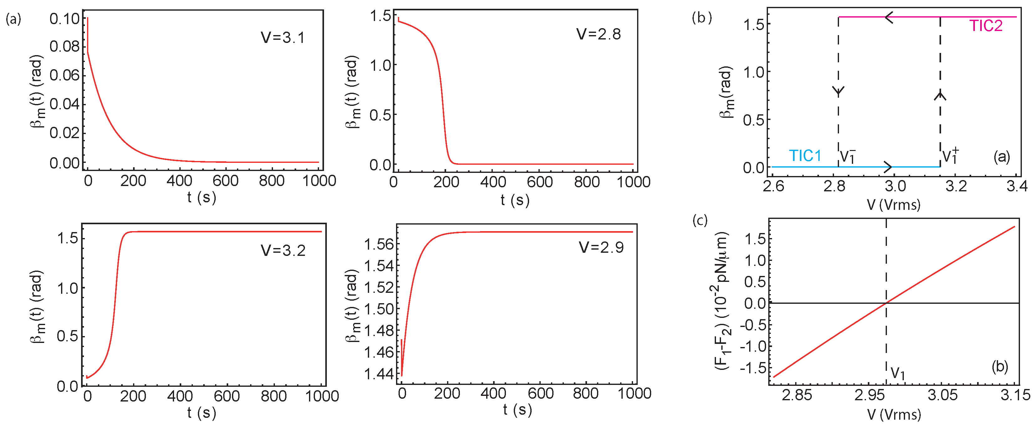
This study is summarized in
Figure A5, which shows a zoom of the phase diagram around the tricritical point in the parameter plane
. In this figure, the base line
corresponds to the spinodal line of the HN. The two blue dashed lines and the red solid line are, respectively, the spinodal lines and the coexistence line of the transition between the two TICs on the left of the tricritical point TCP and between the TIC and the NH on the right of this point. Note that the point TCP is at the intersection of this coexistence line and the spinodal line of the HN and has for coordinates (
m,
). We add that the existence of the critical point is not linked to the presence of the magnetic field since it also exists at field
B = 0. On this subject, we refer to the theoretical article by Gartland et al. [
20] where this result is rigorously demonstrated in the case
.
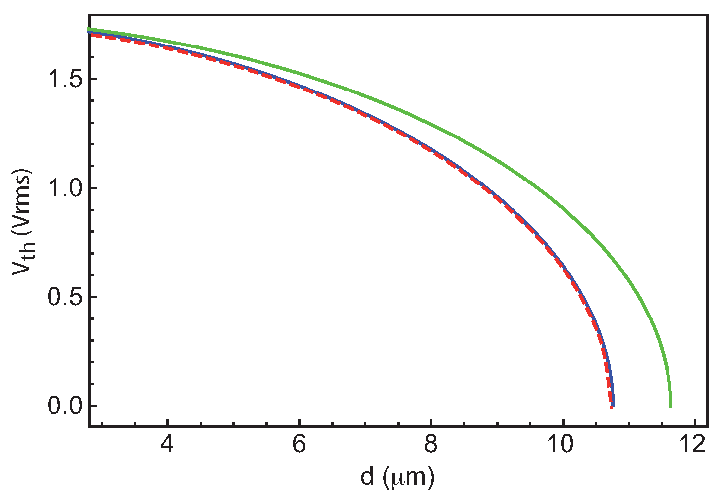
To conclude this study, we calculated the amplitude of the TIC on the spinodal curve
of the HN at large thicknesses when
d approaches
, the thickness at which
vanishes. By choosing
or
Vrms as before, we found systematically a TIC oriented parallel to
B between
and a thickness
m. By contrast, by taking
Vrms, we observed for thicknesses larger than a thickness
m, a second branch of solution, corresponding to a TIC oriented perpendicular to
B (
). This TIC (TIC2) has a larger amplitude than the TIC parallel to
B (TIC1) as shown in
Figure A6a. By calculating the energy of these two TIC [see
Figure A6b], we found that TIC1 has less energy than TIC2 when
m and, conversely, that TIC2 has less energy than TIC1 when
.
Figure A5.
Phase diagram in the vicinity of the tricritical point (TCP). On the left of TCP, two transitions are observed as a function of the voltage: a second order transition between the HN and a TIC of small amplitude and a first order transition between two TIC of non-zero amplitudes. This transition ends at the critical point CP (cusp point). On the right of the tricritical point, a first order transition between the HN and a TIC of large amplitude is observed.
Figure A6.
Maximal tilt angle (a) and energy (b) of TIC1 and TIC2 solutions as a function of the thickness calculated on the spinodal line of the HN when . The two solutions coexist between and and have the same energy at . When , TIC1 forms (TIC parallel to B), while TIC2 is preferred when (TIC perpendicular to B).


