
Basic Modelling of General Strength and Creep Properties of Alloys

Materials Science and Engineering, KTH Royal Institute of Technology, SE-10044 Stockholm, Sweden
Crystals 2024, 14(1), 21; https://doi.org/10.3390/cryst14010021
Submission received: 30 November 2023
/
Revised: 12 December 2023
/
Accepted: 21 December 2023
/
Published: 25 December 2023
(This article belongs to the Special Issue Feature Papers in Crystals 2023)
Abstract
:There are excellent methods for modelling physical and elastic properties, for example, those based on ab initio atomistic procedures. For mechanical properties that are controlled by the motion of the dislocations, such methods have not been available in the past. One has been forced to resort to fitting the experimental data with empirical methods by involving a number of adjustable parameters. However, in recent years, methods based on physical principles have been developed for a number of mechanical properties. These methods can predict properties accurately without the use of fitting parameters. A review of such methods will be given, for example, for the modelling of creep deformation in metallic materials. It will be demonstrated that some properties can be described over a wide range of temperatures and strain rates. The advantage of these new methods is that they can be used for prediction, identification of mechanisms and extrapolation of results for new conditions.
1. Introduction
In recent years, rapid progress has taken place for the basic modelling of properties. Perhaps the most striking development is with quantum mechanics (ab initio) calculations. The full many-body problem cannot be solved. However, there are excellent approximate procedures such as density functional theory (DFT), and practical computations can be readily performed. By minimising the energy of atomic systems, the crystal structure and lattice parameters can be predicted [1]. With the help of the modelled electronic structure, successful modelling of many physical properties has been performed. Examples are electric and thermal conductivity [2,3], surface properties [4,5] and elastic constants [6]. The virtue of this type of modelling is that no adjustable parameters are involved and no calibration for observations are needed. This is most important because it makes it possible to make predictions also for systems and cases, where no measurements have been performed. For these reasons, this type of computation is referred to as fundamental.
Another area where basic predictions can be made is in the field of thermodynamics (computational thermodynamics, CTD). The first step is to model the free energy of systems where predictions should be made. The free energy is described with a range of parameters that are fitted to properties like specific heat. This step is not fundamental since it involves adjustable parameters. But once the models for the free energy are established, fixed and collected in the thermodynamic databases, the free energy models can be used for predictions without involving any new adjustable parameters. This approach is called Calphad since it was first used to compute phase diagrams. The prediction of lattice structures and the content of alloying elements in and out of solid solutions is still one of the main applications of the systems. If combined with diffusion data, many types of microstructural changes such as precipitation, coarsening and dissolution of particles can be analysed and predicted. Since the predictions can be made without introducing new adjustable parameters, this type of computation is referred to as basic.
For mechanical properties, the situation is different. Only limited efforts for basic modelling have been performed so far in comparison to those with ab initio methods and CTD. However, for example, for time-dependent mechanical properties (creep), important results have been obtained [7]. The strength, ductility and toughness of alloys are controlled by dislocation mechanisms, and this makes basic modelling less straightforward. Mechanical properties have traditionally been handled with empirical models that have been fitted to experimental data with the help of adjustable parameters. The concept of basic modelling can mean different things to different researchers. To be precise, in the present paper, a basic model is one that can give a good description of observations without using adjustable parameters or somehow calibrating the model to the experiments, and it is derived from basic physical principles.
The probably most common way of measuring mechanical properties is with a tensile test, where a stress–strain curve is generated. Strength values are obtained as yield and tensile strength and ductility results as elongation and reduction in area. The modelling of stress–strain curves is almost exclusively performed with empirical methods. Hollomon, Ludwik and Voce are well-known models that are named after the person that first proposed them (for references to the original papers, see [8]). These models are simple mathematical expressions with two to three adjustable parameters. These models were proposed without any physical background. The only model that later has been possible to give a physically based derivation is that of Voce. This will be described in Section 3.
Since mechanical properties are governed by dislocation mechanisms, the dislocation structure must be precisely modelled. The starting point in this paper is an equation for the development of the dislocation density as a function of strain or time. There are three main contributions to the dislocation density: work hardening, dynamic recovery and static recovery. Basic models for these processes have been possible to derive for poly-crystals that are valid for FCC and BCC alloys. They will be described in Section 2. During all types of deformation, there is a competition between the generation (work hardening) and annihilation (recovery) of dislocations. During heat treatment, recovery is the dominating process. It is assumed that the models’ work hardening and recovery are general. It has been shown that they are able to describe strain-controlled and time-controlled deformation, as well as fatigue [9,10].
Both empirical and basic models can be quite valuable. In general, empirical models are presented first for a new phenomenon. They can often describe the experiments in a straightforward way. Later, when more has been learned about the phenomenon, semi-empirical or basic models are developed. One classical example is Bohr’s well-known empirical model for the hydrogen atom, where an electron is circulating around a proton. The model was superseded by a quantum mechanics model. Bohr’s model inspired a number of experiments and physical thinking and was very useful at the time. Nevertheless, with the fundamental quantum mechanics model, accurate predictions can be made. These are characteristics of the difference between empirical and basic models. Empirical models are simple to formulate and apply, but it is very difficult or impossible to generalise and extrapolate them for new conditions or new alloys, which is practically always desirable. Basic models are typically more difficult to derive, but the models can be applied even to systems where no experiments have been performed.
2. Dislocation Model
During deformation, new dislocations are continuously generated. Since the dislocations contribute to the strength, often the most important contribution, the generation of dislocations is referred to as work hardening. However, the generation of dislocations is not the only process active during deformation. If it were, the stress–strain curve would be straight, as for a brittle ceramic. However, with increasing stress, the dislocations are annihilating each other to quite some extent and this gives a curved stress–strain curve. This is illustrated in Section 3. Thus, the work hardening and the recovery processes are vital. Since the dislocation model is fundamental for the prediction of properties, a brief derivation of it will be given.
The expression for the work hardening is based on the Orowan equation [11]:
is the deformation rate, b is Burgers vector, is the dislocation density, v is the velocity of the dislocations, and mT is the Taylor factor [12] that takes into account the translation from shear strains to tensile strains. Equation (1) is based on simple geometry of the deformation and is general. If Equation (1) is integrated, one obtains the following:
Plastic deformation takes place by the release of dislocations that travel, on average, a distance Ls, the spurting distance. If Equation (2) is derived and Ls is kept constant, the expression for work hardening is obtained as follows:
The spurt distance can be related to barriers in the material. Ls is controlled by the cell boundaries. The cell boundaries consist of dislocation networks that divide the material into a cell structure that is also called a substructure. Ls is assumed to be approximately equal to the cell diameter dsub.
It might be thought that the spurting dislocations are fully stopped by the cell boundaries, which would give nsub = 1. However, it has been observed experimentally that dislocations can pass through at least one or two cell boundaries, implying that nsub = 1 to 3. The cell size dsub is related to the dislocation density according to a classical equation. For a derivation, see [13].
The constant Ksub has a value of about 10 [14]. The theoretical value of the constant α is 0.19 [15]. Combining Equations (1) and (2) gives the following equation:
Together with Equation (3), the following expression for the work hardening is obtained:
With mT = 3.06 [12], one finds that cL is about 35, which is accurate enough for a number of applications. However, for the stress–strain curves that are considered in Section 3, a more accurate value for cL is needed. Equation (7) is also a common representation of work hardening in empirical models; see for example [16,17].
When dislocations of opposite Burgers vectors become close together, they can form a low energy configuration or annihilate each other. This is referred to as dynamic recovery. This process is taken into account with the following equation:
ω is referred to as the dynamic recovery constant. Equation (8) and the value of ω was derived by Roters et al. [18]
dint is the distance where the interaction takes place and nslip is the number of slip systems (for FCC alloys nslip = 12). The value of dint is quite small [19]. In fact, dislocations have to touch each other before any annihilation can occur. Take copper as an example. According to ab initio calculations, the core radius is 1.3 b [20], which gives dint = 2.6 b. Inserting this value into Equation (9), ω = 15 is obtained in good agreement with observations. The combination of Equations (7) and (8) are commonly used to describe stress curves both in basic [21] and empirical work [22,23]. A list of other similar papers can be found in [24].
Dislocations on a given slip plane with opposite Burgers’ vectors attract each other, and if they are free to move, they will eventually annihilate each other. The change in the dislocation density can be described by the following equation:
t is the time, L the dislocation line tension, and Mcl the dislocation climb mobility. The reduction in the dislocation density is time-based, meaning that it does not only occur during deformation but also during heat treatment. The idea behind Equation (10) was suggested by Friedel [25], but he never gave any derivation of it. Lagneborg and co-workers [26] were the first to make extensive use of it. To derive Equation (10), a network of dislocations with an average spacing of R will be considered. Two screw dislocations of opposite sign will attract each other according to the following equation:
where G is the shear modulus. In the second equality, the stress from a neighbouring screw dislocation is introduced. In the third equality, the expression L = Gb2/2 for the line tension of a dislocation is introduced. If edge or mixed dislocations are involved instead, the result is the same. The time telim that it takes to eliminate one pair of dislocations is obtained after integrating the last member of Equation (11).
Differentiation of Equation (12) with respect to time yields the following equation:
This equation describes the recovery of dislocation. If now, the relation R = is applied to Equation (13), Equation (10) is recovered.
The derivation above is limited to a pair of dislocations. To illustrate the behaviour for a network of dislocations, dislocation dynamics simulations have been performed. Randomly distributed parallel dislocations have been considered with six different Burgers vectors; see Figure 1. Edge dislocations are represented with four sets (top, bottom, left, right) and screw dislocations with two (down, up). Dislocations of opposite signs (top, bottom), (left, right) and (down, up) attract each other and eventually annihilate each other.
The findings of the simulations are shown in Figure 2. It can be seen that the results agree quite well with Equation (10). The validity of this equation is obviously not restricted to a single pair of dislocations.
Combining Equations (7), (8) and (10) gives the full equation for the dislocation density, as follows:
In the final term of Equation (14), the chain rule for the derivative has been used:
The three terms of the RHS of Equation (14) represent work hardening, dynamic recovery and static recovery. The equation is not fully general for polycrystalline alloys. It works well for FCC alloys. However, for some materials like martensitic steels, more than one type of dislocation density has to be taken into account. This means that a system of equations of the same type as in Equation (14) has to be formulated [27].
3. Stress–Strain Curves
3.1. Empirical Models
Since empirical models are discussed a number of times in this paper, a few examples will be given for stress–strain curves. Stress–strain curves are, for example, obtained in ordinary tensile tests. Examples for the austenitic 17Cr12Ni2Mo stainless steel 316H at room temperature and at 800 °C are shown in Figure 3.
A number of empirical expressions to represent stress–strain curves can be found in the literature. Some of the classical methods are those of Ludwik, Hollomon, Voce and Swift. The equations are listed in Equations (16)–(19). References to the original papers are given in [8].
σ is the stress and ε is the strain. The remainder of the quantities are adjustable parameters that are fitted to the data. Equations (16)–(19) are applied in Figure 3. The methods of Ludwik, Voce and Swift provide a satisfactory representation in Figure 3a at room temperature but not that of Hollomon. On the other hand, at 800 °C, in Figure 3b, three of the approaches work well but not Voce’s method.
However, the deficiencies are easily fixed by including more adjustable parameters. One way is to combine the Ludwik and Voce methods, as follows:
Another way is to duplicate the approaches:
The use of these extended expressions is illustrated in Figure 4. Now, satisfactory fits are obtained both at room temperature and at 800 °C.
There are characteristic features of empirical models. The models discussed above were all proposed just to be able to fit stress–strain curves and none had any physical background. Only one method, the Voce method, has later been possible to give a basic derivation, which is shown in Section 3.2. By generalising the expression and increasing the number of adjustable parameters, the fits can naturally be improved. A characteristic feature of empirical models is that it is typically not possible in advance to identify the model that gives the best representation of the experimental data, since it depends on the material and the testing conditions. It is also obvious that empirical models are of little value for identifying operating mechanisms.
3.2. Basic Model
In this section, a basic derivation will be given for the Voce Equation (18). The derivation will be based on Equation (14) for the strain dependence of the dislocation density. At ambient and modestly high temperature, it can be shown that the last term in Equation (14), the static recovery term, is typically small and can be neglected. This will be illustrated below. Neglecting the static recovery term, Equation (14) can be integrated directly:
The Taylor equation is used to compute the strength from the dislocations [16]:
where σdisl is the strength contribution from the dislocations, σy is the yield strength, α = 0.19, a theoretically derived constant [15,28], and G is the shear modulus. The strain dependence of the strength is obtained by combining Equations (23) and (24).
The maximum stress in Equation (25) is called the saturation stress σsat.
Equation (27) has precisely the form of the Voce Equation (18).
Equation (14) without the last term has been applied for many years to derive the Voce equation [16,22,23]. However, in these papers, a number of adjustable parameters were involved. But that is no longer necessary. The parameters are based on theoretically derived values, except for the yield strength that is batch-dependent in a way that cannot be predicted at present. For the yield strength, it is consequently necessary to use experimental values.
The temperature dependence of the yield strength is approximately proportional to that of the shear modulus G(T), which is often linear in temperature.
In Figure 5, the model in Equation (25) is applied to stress–strain curves for pure Cu with 50 ppm P, Cu-OFP. The slope of the curves represents the work hardening, which is approximately constant at low strains. With increasing strain, there is a gradual decrease in the work hardening. The modelled stress–strain curves eventually reach a maximum value, σsat, in Equation (26). The measured tensile stress–strain curves cannot cover large strains since necking takes place, where the engineering stress starts to fall rapidly.
When computing the model curves in Figure 5, the last term in Equation (14), the static recovery term, was ignored. The justification for this is illustrated in Figure 6. If static recovery is taken into account, the saturation stress is lowered. Since the climb mobility in the static recovery term is proportional to the diffusion coefficient, the contribution from the term increases with temperature. Thus, the influence on the static recovery is much less in Figure 5 than in Figure 6 because of the lower temperature in Figure 5. When stress–strain flow curves are determined at a higher temperature, they often have the appearance of the ‘static recovery’ curve in Figure 6. At larger strains, a stationary stress appears that is typical when creep is the dominating deformation mechanism.
4. Stationary Creep
4.1. Basic Model for Stationary Creep
In the common form of creep strain testing, a specimen is exposed to a constant load or stress while the amount of strain is recorded. The creep straining is usually divided into three stages: primary, secondary and tertiary [29]. The typical behaviour is that the strain rate (creep rate) is high in the primary stage but continuously slows down until the secondary stage is reached, where the strain rate is constant. This situation prevails until the tertiary stage is entered, when the strain rate is increased. Many studies are focussed on the secondary stage because it gives a well-defined creep rate as a function of stress and temperature [19]. The secondary stage is also referred to as the stationary stage, since the creep rate is approximately constant.
The present paper only considers dislocation creep. At sufficiently high temperatures, diffusion creep where the creep deformation takes place by diffusion of vacancies is expected to be of importance. However, it has been known for many years that diffusion creep can be strongly overestimated by the classical models [30,31]. For example, according to the Coble creep model (diffusion along grain boundaries), diffusion creep should be dominating in austenitic stainless steels at stresses of around 50 MPa at 700 °C, but that has not been found experimentally [32]. In two recent studies, it has been demonstrated that dislocation creep can be the controlling mechanism even if the stress dependence of the secondary creep rate has an exponent of 1 [32,33]. These findings make it more difficult to find out where diffusion creep is of importance, and for this reason, it is not taken up in this paper.
Sometimes sliding grains (grain boundary sliding, GBS) are introduced as a separate mechanism parallel to dislocation creep. GBS can be a dominating mechanism during superplasticity [34]. However, it is shown in recent, still unpublished work by the author that basic models for GBS based on dislocation creep can be derived that can account for observations of superplasticity. Although GBS is important for many phenomena, not least for cavitation [35], there is no need to consider it as a separate mechanism.
The most important characteristic of creep is that the deformation can continue at constant load. This should be contrasted with the deformation behaviour of, for example, steels at ambient temperature. Then, straining only takes place when the load is increased. The basis of the understanding of the creep deformation is the creep recovery theory [26]. It states that there must be a balance between the generation and annihilation of dislocations during secondary creep. Expressed in another way, the rates of work hardening and recovery must be the same. The conditions during secondary creep are assumed to be constant. For example, the dislocation density does not change, and the strain and time derivatives of must vanish. From Equation (14), the secondary creep rate can then be obtained:
To reproduce observations, the contributions from dynamic recovery in Equation (14) are ignored. Taking other strength contributions than those from the dislocation density into account, Equation (24) is reformulated to the following:
σdisl is the dislocation stress. σi is an internal stress that was the yield strength in Equation (24). In alloys, important contributions that come from solid solution hardening and particle hardening must be included in σi. Basic models for the influence of the two mechanisms on the creep deformation are available. The background and history of these models can be found in [36,37]. They have, for example, successfully been applied to austenitic stainless steels [38,39].
Equation (29) can be transferred to stresses with the help of Taylor’s equation (30).
The factor fSFE takes into account the splitting of dislocations into partials. This factor can be related to the stacking fault energy [40].
The mobility Mclimb relates the climb velocity of the dislocations to the applied stress σ.
Glide of dislocations takes place in the slip plane and climb is perpendicular to it. Climb is associated with the emission and absorption of vacancies and is a slower process than glide. Recent findings suggest that dislocation creep is fully controlled by climb [7]. An expression for the climb mobility of metals was derived by Hirth and Lothe [41]:
where T is the absolute temperature, Ds0 is the pre-exponential coefficient for self-diffusion, Qself is the activation energy for self-diffusion, kB is Boltzmann’s constant, and RG is the gas constant.
At low stresses, the climb mobility is almost independent of stress. Together with Equation (31), this gives a creep rate that is proportional to the third power of the stress, which is often formulated as the stress exponent of 3. This behaviour is sometimes referred to as the natural creep law [42], since it is more a less automatically given by the creep recovery theory. A stress exponent of 3 is often found at high temperatures. However, there are many factors that can influence the stress exponent. If creep is controlled by pipe diffusion along the dislocations instead of bulk diffusion, the creep exponent is raised by 2 [43]. The most important contribution comes from strain-induced vacancies. It raises the climb mobility by a factor [7].
4.2. Application to Aluminium
Equation (31) will now be applied to aluminium. The expression (33) for the climb mobility will be used together with Equation (34). A special but small effect has to be taken into account, namely, the Peierls stress, which is usually neglected for FCC metals. Shin and Carter [45] computed the following value for the Peierls stress:
The results for three temperatures are illustrated in Figure 7.
At intermediate stresses, the slope of curves is about 4.5, which corresponds to the stress exponent. At larger stresses, the slope is higher, indicating the start of power law break down. At low stresses, the stress exponent is also higher due to the presence of the Peierls stress.
4.3. Application to Nickel
As pointed out above, the expression for fclglide in Equation (34) works well for Al and Cu. However, for nickel, another expression has been derived [40]:
For Ni at lower temperatures, pipe diffusion must be considered. This is achieved by replacing the expression for bulk diffusion with the following [43]:
where is the dislocation density, Ad is the core area of the dislocations and Dd is the dislocation diffusion coefficient. Using Equations (31), (34), (36) and (37), the creep rate can be computed. The results are compared to experimental data in Figure 8.
With Equation (36), an approximately constant stress exponent of 7 is obtained. There are three contributions to the stress exponent: (1) 3 from Equation (31); (2) 2 from fclglide in Equation (36); and (3) 2 from Equation (37) for pipe diffusion, adding up to 7. It is evident that the basic creep model can describe experimental data for the secondary creep rate of Al and Ni in an acceptable way.
5. Primary Creep
5.1. The 2σ Model
A natural starting point for deriving expressions for primary creep is to modify the expression (31) for the creep rate in the secondary stage. A simple assumption is to use the expression for hsec unchanged and introduce an effective stress. In the so-called 2σ model, the chosen effective stress σeff2σ is [7]:
where σ is the applied stress, σi is the internal stress and σdisl is the dislocation stress, cf. Equation (30). Equation (38) can be slightly generalised to handle tertiary creep as well [48,49], but that will not be covered in the present paper. With the effective stress, the creep rate in the primary stage can be expressed as:
In the beginning of the primary stage, the effective stress can be twice the applied stress, which gives a very high strain rate. Equation (39) is valid also in the secondary stage, where the dislocation stress is given by Equation (30). If this value for the dislocation stress is inserted into Equation (38), Equations (39) and (31) are identical.
Equation (39) is compared to experimental data for Cu with 50 ppm P (Cu-OFP) in Figure 9. In Figure 9a, the creep strain versus time is given. The observed strain on loading is 0.15, in agreement with the model. In Figure 9b, the strain rate versus time is shown. The straight line in the primary stage in the double logarithmic diagram indicates that the ϕ model is satisfied. This model is further discussed in Section 5.2. After about 4000 h, there is a transition in Figure 9 from the primary to the secondary stage. This is most directly seen in Figure 9b, where the slope of the curve is gradually reduced. In the secondary stage, the strain rate takes a constant value. This a consequence of the increase in the dislocation density and thereby the dislocation stress. It is evident from Equation (38) that this implies that the effective stress is reduced and from Equation (39) that the creep rate is lowered. It should be pointed out that no adjustable parameters are involved in the models.
5.2. The Stress Adaption Model
The 2σ model works well at normal stress levels. However, it is not applicable at low stresses. The reason is that the highest stress in the model is twice the applied stress and that turns out to not be enough to cover the full range of creep rates at lower stresses. Fortunately, there is another model that is more suitable at low stresses, which is called stress adaption. A derivation of the model can be found in [33]. It is not very complex, but it will not be repeated here. The difference between the 2σ model and stress adaptation is the effective stress. In stress adaption, it takes the following form:
where σi(T) is the internal stress, including a possible yield strength. K(T) is the difference between the saturation stress σsat and σi, cf. Equation (26). In fact, the parameters in the model are closely related to those in the model for the stress–strain curve. If the time is not too far from the secondary stage, the same parameter values as for the stress–strain curve can be used. For example, Ω is equal to the dynamic recovery constant ω in Equation (23). In the same way as in Equation (39), the creep rate is obtained by inserting the effective stress in the expression for the secondary creep rate:
A simplified version of Equation (41) will be analysed to reveal some of its properties [32]. It is expressed in terms of a Norton equation, with the parameters of the proportionality constant A and the stress exponent n [51]. Assuming small strains, the exponential can be expanded.
This equation is integrated as a function of time:
The time derivative of Equation (43) is:
After integration and derivation, it might be thought that Equations (42) and (44) would be identical, but that is not the case, because Equation (42) is a function of strain and Equation (44) is a function of time.
The stress exponent in Equation (44) is n/(n + 1), which is about 1 if n is not too small. This means that dislocation creep can give a stress exponent as low as 1 during primary creep and be a competing process to diffusion creep. It is shown in Section 5.5 with aluminium that this applies to the full model in Equation (41) as well and not just to the simplified version.
The empirical ϕ model can describe the creep in the primary stage for many materials [33,52].
where t is the time and Aϕ and ϕ are parameters. It is evident from Equation (44) that the stress adaption model follows the ϕ model with a value of ϕ = n/(n + 1). This is also the case for the strain dependence, provided that the following criterion is satisfied:
As pointed out above, under close to stationary conditions, the dynamic recovery constant ω can be used for Ω. The dislocation stress must always be below the applied stress. When the dislocation stress approaches the applied stress, a transition to a semi-stationary stage takes place, where the exponential in Equation (40) must be small. It can be shown that this gives the following value for Ω [33]:
5.3. Cu-OFP at Low Stresses at 95 °C
Ho [53] performed creep tests for Cu-OFP at 95 to 150 °C at stresses from 20 to 100 MPa. The tests were carried for about 5000 h and then interrupted. The measured strain rates at interruption were 3 × 10⁻¹³ to 1.0 × 10⁻¹⁰ 1/s. As will be illustrated below, the tests were never near to stationary conditions. Examples of the test results are shown in Figure 10. The observations are compared to the primary creep model in Equation (41). A comparison is also made to the ϕ model in Equation (45).
These results and similar findings for the other tests carried out by Ho [33] illustrate that the primary creep model can give a good representation of the data. As indicated in Equation (44), the basic equation (41) is in accordance with the ϕ model.
With the help of Equation (31), the stationary creep rate can be estimated for the case in Figure 10. The value found is 1.3 × 10⁻²² 1/s. This is obviously many orders of magnitude lower than the observed creep rate of 3 × 10⁻¹² 1/s. It is clear that the model in Equation (41) can describe the very early stages of primary creep and that the ϕ model is satisfied also under these conditions.
The behaviour of the primary creep model over extended times is illustrated in Figure 11. The creep model follows the ϕ model over many orders of magnitude in time. The model goes towards the constant stationary stress value, when the stationary stage is reached as it should.
The use of the ϕ model is shown in Figure 10 and Figure 11. The ϕ values of the parameter values in the model are selected as the average of the values from the basic model that were found to be in the range from 0.85 to 0.95 [7,54]. The Aϕ values were computed from the following equation:
where the creep rate in the secondary stage is given by Equation (31). tsec is an estimate of when the secondary stage is reached.
The values for εsec = 0.1 at the start of the secondary stage were taken from studies at higher stresses. The results in Figure 10 and Figure 11 show that the simple ϕ model gives a reasonable description of both the creep rate versus time and creep strain versus time.
These results must be considered as astonishing, taking into account the low value of the stationary creep rate. The values in Figure 11 for 125 °C and 40 MPa can be taken as an example. According to the stationary creep model, Equation (31), the stationary creep rate is 1 × 10⁻¹⁸ 1/s and the time to reach the secondary stage is tsec = 3 × 10¹³ h, which is more than 1 million years. It seems evident that a constant ϕ value as well as the primary creep model can represent the data over this extended period of time.
The creep model was originally formulated for Cu-OFP for creep tests at near ambient temperatures at stresses between 150 and 180 MPa, corresponding to creep rates in the interval from 1 × 10⁻¹¹ to 1 × 10⁻⁷ 1/s [19]. The application to the low stresses corresponds to an extrapolation of at least 10 orders of magnitude in the creep rate. Without a basic model, such an extrapolation is not possible.
5.4. Creep of Cu-OFP at 600 °C
The results from the creep test of Cu-OFP (Cu with 54 wt. P) at very low stresses at 600 °C have recently been published [33]. The stresses were chosen as 1, 1.5 and 2 MPa, and the tests were carried out from 12,000 to 17,000 h. This was long enough to reach the secondary stage in at least two of the tests. The original intention was that the stresses were low enough to ensure that diffusion creep would be controlling. However, as will be seen, this did not turn out to be the case. The minimum creep rate is given as a function of stress in Figure 12.
In Figure 12, the stress exponent is 3 for the experimental data. The experiments are compared to the model for stationary creep in Equation (31). The model gives a stress exponent of 4 for Cu-OFP and 3 for Cu-OF (pure Cu without P). How the influence of P is taken into account is described in [7]. With an experimental creep exponent of 3 and a dislocation model than can reproduce the data, it is clearly shown that dislocation creep is the controlling mechanism. This is in spite of the fact that diffusion creep in the grain boundaries (Coble creep) gives a significantly higher creep rate (Figure 12b). Diffusion creep in the bulk (Herring–Nabarro creep) yields a creep rate of the right order of magnitude but with the wrong stress exponent of 1. A possible mechanism to explain why Coble creep can overestimate the observed creep rates can be that the deposition of material that takes place at the grain boundaries cannot occur without accompanying creep in the bulk. This means that the Coble creep rate cannot be significantly faster than the bulk creep rate. This phenomenon is referred to as constrained boundary creep [32,33].
In Figure 13, the results for the creep in the primary stage are compared to the stress adaption model in Equation (41). The room temperature values of σy and K available in [55] are chosen. The Ω value is selected according to Equation (47). It is also ensured that the criterion (46) is satisfied.
The ϕ model is followed except when the stationary stage is reached and a constant strain rate is obtained. At 2 MPa, the stationary creep rate is somewhat overestimated. This is evident already from Figure 12. Again, a reasonable representation of the experimental data has been obtained.
5.5. Aluminium at Low Stresses; Harper–Dorn Creep
Harper and Dorn investigated creep in aluminium at very high temperatures and low stresses in an attempt to observe diffusion creep [56]. They obtained a stress exponent of 1 that is a characteristic feature of both Coble and Nabarro–Herring creep. However, the observed creep rate was two orders of magnitude higher that of Nabarro–Herring. They suggested that a new form of dislocation creep had been found. Since coarse-grained aluminium was studied, Coble creep was not of importance. The findings of Harper–Dorn have been widely debated and a number of attempts have been made to reproduce the results that are now referred to as Harper–Dorn creep. In two more recent papers, available data have been reanalysed [57,58]. One suspicion was that the creep tests had not been of sufficient length to reach the secondary stage. For this reason, Kumar et al. [58] carried out new longer tests. They found a stress exponent of 3, clearly demonstrating that ordinary dislocation creep is involved. Several sets of published data were consistent with these observations, including the data of Harper and Dorn, if an assumed threshold stress was removed.
Some of the observations show a lower stress exponent than 3. A possibility is that the stationary stage had not been reached in these cases. To investigate that, these results will be compared to the primary creep model in Equation (41).
Harper–Dorn creep is near to stationary conditions. A value of Ω = 40 is chosen, which is the temperature-corrected value from the stress–strain curves. For σy(T)/K(T), a ratio of 0.01 has been selected that fulfils the criterion (46). As long as this value is small, it does not influence the results much, cf. Equation (44).
In Figure 14, comparisons are made to the experimental data for both stationary and primary creep. The stationary creep model, Equation (31), giving a stress exponent of 3 is in good accordance with most of the data. In two of the data sets, attempts were made to ensure that stationary conditions had been reached [58,59]. These data are close to the stationary curve. Most of the tests had a duration of up to 1000 h. However, there are some data that lie above the stationary creep curves. In one series, Ginter et al. [59] purposely used a shorter testing time of 200 h to try to stay in the primary stage. These data marked as reduced are indeed located above the stationary curves. In the three remaining sets [56,60,61], the testing times were not specified, and it can be assumed that they represent data in the primary stage. They are also located above the stationary curve. In the diagram, predicted curves for primary creep of length between 68 and 938 h are included. The data deviate from the stationary curve below 0.2 MPa. In this range, the results clearly overlap with the data that are expected to be in the primary creep range.
In Figure 14, the predicted stress dependence of Nabarro–Herring creep is given. It is well below the stationary creep line. A grain size of 1 mm has been assumed. In the various investigations mentioned above, a coarse grain structure has been chosen to avoid influence from diffusion creep.
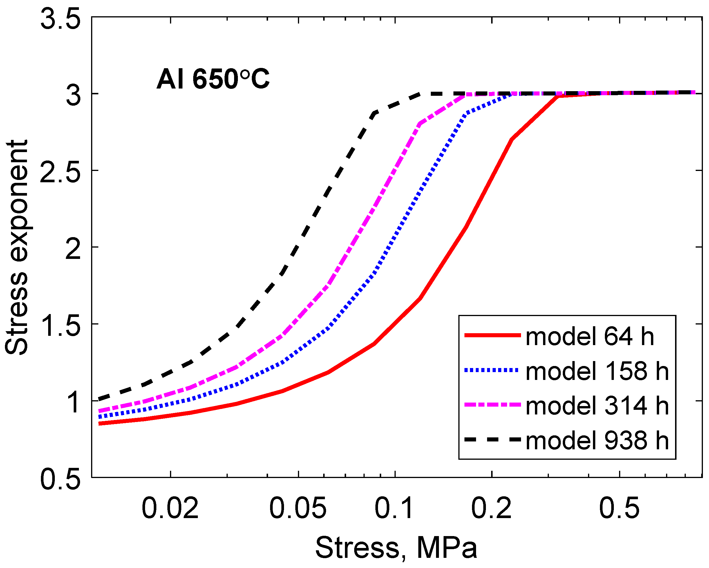
The stress exponent that is predicted from the primary creep model, Equation (41), is illustrated Figure 15 as a function of stress at the four testing times considered in Figure 14. At very low stresses, a stress exponent of about 1 is found. This is also the case for two of the test sets in Figure 14. Above a stress of 0.08 to 0.3, the secondary stage is reached at the analysed testing times, giving a stress exponent of 3. It is evident that dislocation creep in the primary stage can give a stress exponent of about 1, in agreement with Equation (44).
6. Discussion
The main purpose of this review paper is to show that accurate prediction of mechanical properties can be made. The models must be based on fundamental physical principles. An essential ingredient is also that the use of adjustable parameters is avoided. The most important effect of this is that basic models can be derived which are valid over a wide range of conditions. This will now be quantified for creep of Cu.
Basic models for creep of copper were first developed for conditions at near ambient temperatures at high stresses [7,19]. Models for both primary and secondary creep were established. In Section 5.2, data for creep at low stresses at 600 °C were analysed. The same high-stress models were successfully applied in this case. This represents a very large extrapolation both in terms of stress and temperature. This is illustrated for the secondary creep rate in Table 1. Ratios for stress changes are given as the creep rate at the high stress value divided by that at the low stress value. The corresponding ratios for temperature changes are shown as the creep rate at the high temperature divided by that at the low one. The stress change ratios depend on the temperature, and the temperature change ratios are a function of the stress. The precise creep rate ratios are not very important but their very high values of 10 orders of magnitude or more demonstrate that the models can handle a wide range of conditions.
The results in Table 1 are not unique. We saw in Section 5.3 for Cu-OFP at 95 °C that the stress changes could cope with a creep rate ratio of 1 × 10¹⁰. A table similar to Table 1 can be set up for aluminium [32]. The resulting stress change and temperature change creep ratios are quite similar to those in Table 1. The most important consequence of the high extrapolation ratios is that they verify the accuracy of the basic models.
Accurate modelling of the mechanical properties of alloys is thus possible without involving adjustable parameters. To mention just a few other examples, precipitation hardening has been handled for CuCo alloys [37] and austenitic stainless steels [62], solid solution hardening for aluminium alloys [7] and austenitic stainless steels [36], and ductile and brittle rupture for austenitic stainless steels [38,39]. However, much more remains to be accomplished.
7. Conclusions
In the paper, models that can accurately describe mechanical properties without involving adjustable parameters are reviewed. The derivation of the models is based on basic physical principles.
The starting point is a model for the development of the dislocation density describing the effect of work hardening and recovery. From the dislocation model, expressions for stress–strain curves and for the temperature and stress dependence of the creep strain rate can be derived.
The basic models for mechanical properties can be made valid for a wide range of conditions and can be generalised and extrapolated. This is verified for creep models of primary or secondary creep. They can reproduce data at low and high temperatures as well as low and high stresses, representing an extrapolation of the creep rate by 10 orders of magnitude or more.
A better direct verification of the basic models and their wide applicability is difficult to find.
Funding
This research did not receive any specific grant from funding agencies in the public, commercial or not-for-profit sectors.
Data Availability Statement
The data required to reproduce these findings are available on request.
Conflicts of Interest
The author declares no conflict of interest.
References
- Ikeda, Y.; Grabowski, B.; Körmann, F. Ab initio phase stabilities and mechanical properties of multicomponent alloys: A comprehensive review for high entropy alloys and compositionally complex alloys. Mater. Charact. 2019, 147, 464–511. [Google Scholar] [CrossRef]
- Ladha, D.G. A review on density functional theory–based study on two-dimensional materials used in batteries. Mater. Today Chem. 2019, 11, 94–111. [Google Scholar] [CrossRef]
- Zhang, Y. First-principles Debye–Callaway approach to lattice thermal conductivity. J. Mater. 2016, 2, 237–247. [Google Scholar] [CrossRef]
- De Luca, G.; Basile, A. 17—Assessment of the key properties of materials used in membrane reactors by quantum computational approaches. In Handbook of Membrane Reactors; Woodhead Publishing: Sawston, UK, 2013; pp. 598–626. [Google Scholar]
- Maurice, V.; Marcus, P. Passive films at the nanoscale. Electrochim. Acta 2012, 84, 129–138. [Google Scholar] [CrossRef]
- David, M.; Prillieux, A.; Monceau, D.; Connétable, D. First-principles study of the insertion and diffusion of interstitial atoms (H, C, N and O) in nickel. J. Alloys Compd. 2020, 822, 153555. [Google Scholar] [CrossRef]
- Sandström, R. Fundamental Models for the Creep of Metals. In Creep; IntechOpen: London, UK, 2017. [Google Scholar]
- Choudhary, B.K.; Samuel, E.I.; Rao, K.B.S.; Mannan, S.L. Tensile stress–strain and work hardening behaviour of 316LN austenitic stainless steel. Mater. Sci. Technol. 2001, 17, 223–231. [Google Scholar] [CrossRef]
- Sandström, R. Cavitation during creep-fatigue loading. Mater. High Temp. 2023, 40, 174–183. [Google Scholar] [CrossRef]
- Sandström, R. Basic Creep-Fatigue Models Considering Cavitation. Trans. Indian Natl. Acad. Eng. 2022, 7, 583–591. [Google Scholar] [CrossRef]
- Orowan, E. Fracture and strength of solids. Rep. Prog. Phys. 1949, 12, 185–232. [Google Scholar] [CrossRef]
- Kocks, U.F. The relation between polycrystal deformation and single-crystal deformation. Met. Mater. Trans. 1970, 1, 1121–1143. [Google Scholar] [CrossRef]
- Kuhlmann-Wilsdorf, D.; Van Der Merwe, J. Theory of dislocation cell sizes in deformed metals. Mater. Sci. Eng. 1982, 55, 79–83. [Google Scholar] [CrossRef]
- Staker, M.R.; Holt, D.L. The dislocation cell size and dislocation density in copper deformed at temperatures between 25 and 700Â °C. Acta Metall. 1972, 20, 569–579. [Google Scholar] [CrossRef]
- Orlová, A. On the relation between dislocation structure and internal stress measured in pure metals and single phase alloys in high temperature creep. Acta Met. Mater. 1991, 39, 2805–2813. [Google Scholar] [CrossRef]
- Kocks, U.F. Laws for Work-Hardening and Low-Temperature Creep. J. Eng. Mater. Technol. Trans. ASME 1976, 98, 76–85. [Google Scholar] [CrossRef]
- Roberts, W.; Bergström, Y. The stress-strain behaviour of single crystals and polycrystals of face-centered cubic metals—A new dislocation treatment. Acta Met. 1973, 21, 457–469. [Google Scholar] [CrossRef]
- Roters, F.; Raabe, D.; Gottstein, G. Work hardening in heterogeneous alloys—A microstructural approach based on three internal state variables. Acta Mater. 2000, 48, 4181–4189. [Google Scholar] [CrossRef]
- Sandström, R. Basic model for primary and secondary creep in copper. Acta Mater. 2012, 60, 314–322. [Google Scholar] [CrossRef]
- Wang, R.; Wang, S.; Wu, X. Edge dislocation core structures in FCC metals determined from ab initio calculations combined with the improved Peierls-Nabarro equation. Phys. Scr. 2011, 83, 045604. [Google Scholar] [CrossRef]
- Sandström, R.; Hallgren, J. The role of creep in stress strain curves for copper. J. Nucl. Mater. 2012, 422, 51–57. [Google Scholar] [CrossRef]
- Bergström, Y. A dislocation model for the stress-strain behaviour of polycrystalline α-Fe with special emphasis on the variation of the densities of mobile and immobile dislocations. Mater. Sci. Eng. 1970, 5, 193–200. [Google Scholar] [CrossRef]
- Bergström, Y.; Roberts, W. A dislocation model for dynamical strain ageing of α-iron in the jerky-flow region. Acta Met. 1971, 19, 1243–1251. [Google Scholar] [CrossRef]
- Mohamadnejad, S.; Basti, A.; Ansari, R. Analyses of Dislocation Effects on Plastic Deformation. Multiscale Sci. Eng. 2020, 2, 69–89. [Google Scholar] [CrossRef]
- Friedel, J. Dislocations; Addison-Wesley: Reading, MA, USA, 1964. [Google Scholar]
- Lagneborg, R. Dislocation mechanisms in creep. Int. Metall. Rev. 1972, 17, 130–146. [Google Scholar] [CrossRef]
- Magnusson, H.; Sandström, R. Creep Strain Modeling of 9 to 12 Pct Cr Steels Based on Microstructure Evolution. Met. Mater. Trans. A 2007, 38, 2033–2039. [Google Scholar] [CrossRef]
- Lavrentev, F. The type of dislocation interaction as the factor determining work hardening. Mater. Sci. Eng. 1980, 46, 191–208. [Google Scholar] [CrossRef]
- Evans, R.W.; Wilshire, D. Creep of Metals and Alloy; Institute of Metals: London, UK, 1985. [Google Scholar]
- Herring, C. Diffusional Viscosity of a Polycrystalline Solid. J. Appl. Phys. 1950, 21, 437–445. [Google Scholar] [CrossRef]
- Coble, R.L. A Model for Boundary Diffusion Controlled Creep in Polycrystalline Materials. J. Appl. Phys. 1963, 34, 1679–1682. [Google Scholar] [CrossRef]
- Sandström, R. Creep at low stresses in aluminium (Harper-Dorn) and in an austenitic stainless steel with a stress exponent of 1. Mater. Today Commun. 2023, 36, 106558. [Google Scholar] [CrossRef]
- Sandström, R. Primary creep at low stresses in copper. Mater. Sci. Eng. A 2023, 873, 144950. [Google Scholar] [CrossRef]
- Langdon, T. A unified approach to grain boundary sliding in creep and superplasticity. Acta Met. Mater. 1994, 42, 2437–2443. [Google Scholar] [CrossRef]
- Sandström, R.; He, J. Survey of Creep Cavitation in fcc Metals. In Study of Grain Boundary Character; IntechOpen: London, UK, 2017. [Google Scholar]
- Korzhavyi, P.; Sandström, R. First-principles evaluation of the effect of alloying elements on the lattice parameter of a 23Cr25NiWCuCo austenitic stainless steel to model solid solution hardening contribution to the creep strength. Mater. Sci. Eng. A 2015, 626, 213–219. [Google Scholar] [CrossRef]
- Sui, F.; Sandström, R. Creep strength contribution due to precipitation hardening in copper–cobalt alloys. J. Mater. Sci. 2019, 54, 1819–1830. [Google Scholar] [CrossRef]
- He, J.; Sandström, R. Application of Fundamental Models for Creep Rupture Prediction of Sanicro 25 (23Cr25NiWCoCu). Crystals 2019, 9, 638. [Google Scholar] [CrossRef]
- He, J.; Sandström, R. Basic modelling of creep rupture in austenitic stainless steels. Theor. Appl. Fract. Mech. 2017, 89, 139–146. [Google Scholar] [CrossRef]
- Sandström, R.; Zhang, J. Modeling the Creep of Nickel. J. Eng. Mater. Technol. 2021, 143, 041011. [Google Scholar] [CrossRef]
- Hirth, J.P.; Lothe, J. Theory of Dislocations; Krieger: Malabar, FL, USA, 1982. [Google Scholar]
- Blum, W.; Eisenlohr, P.; Breutinger, F. Understanding creep—A review. Metall. Mater. Trans. A Phys. Metall. Mater. Sci. 2002, 33, 291–303. [Google Scholar] [CrossRef]
- Ruano, O.A.; Miller, A.K.; Sherby, O.D. The influence of pipe diffusion on the creep of fine-grained materials. Mater. Sci. Eng. 1981, 51, 9–16. [Google Scholar] [CrossRef]
- Spigarelli, S.; Sandström, R. Basic creep modelling of aluminium. Mater. Sci. Eng. A 2018, 711, 343–349. [Google Scholar] [CrossRef]
- Shin, I.; Carter, E.A. Possible origin of the discrepancy in Peierls stresses of fcc metals: First-principles simulations of dislocation mobility in aluminum. Phys. Rev. B-Condens. Matter Mater. Physic 2013, 88, 064106. [Google Scholar] [CrossRef]
- Servi, I.S.; Grant, N.J. Creep and stress rupture behaviour of aluminium as a function of purity. Trans. AIME 1951, 191, 909–916. [Google Scholar]
- Norman, E.; Duran, S. Steady-state creep of pure polycrystalline nickel from 0.3 to 0.55 Tm. Acta Met. 1970, 18, 723–731. [Google Scholar] [CrossRef]
- Sui, F.; Sandström, R. Basic modelling of tertiary creep of copper. J. Mater. Sci. 2018, 53, 6850–6863. [Google Scholar] [CrossRef]
- Sandström, R. Basic Analytical Modeling of Creep Strain Curves. Materials 2023, 16, 3542. [Google Scholar] [CrossRef] [PubMed]
- Sandström, R. The role of cell structure during creep of cold worked copper. Mater. Sci. Eng. A 2016, 674, 318–327. [Google Scholar] [CrossRef]
- Norton, F.H. The Creep of Steel at High Temperatures; McGraw-Hill Book Co.: New York, NY, USA, 1929. [Google Scholar]
- Wu, R.; Sandström, R.; Seitisleam, F. Influence of Extra Coarse Grains on the Creep Properties of 9 Percent CrMoV (P91) Steel Weldment. J. Eng. Mater. Technol. 2004, 126, 87–94. [Google Scholar] [CrossRef]
- Ho, E.T.C. A Study of Creep Behaviour of Oxygen-Free Phosphorus-Doped Copper under Low-Temperture and Low-Stress Test Conditions. In Report No: 06819-REP-01200-10031-R00; Ontario Power Technologies: Toronto, ON, Canada, 2000. [Google Scholar]
- Sandström, R. Formation of a dislocation back stress during creep of copper at low temperatures. Mater. Sci. Eng. A 2017, 700, 622–630. [Google Scholar] [CrossRef]
- Sandstrom, R. Extrapolation of Creep Strain Data for Pure Copper. J. Test. Eval. 1999, 27, 31–35. [Google Scholar]
- Harper, J.; Dorn, J. Viscous creep of aluminum near its melting temperature. Acta Met. 1957, 5, 654–665. [Google Scholar] [CrossRef]
- Kassner, M.E.; Kumar, P.; Blum, W. Harper–Dorn creep. Int. J. Plast. 2007, 23, 980–1000. [Google Scholar] [CrossRef]
- Kumar, P.; Kassner, M.E.; Blum, W.; Eisenlohr, P.; Langdon, T.G. New observations on high-temperature creep at very low stresses. Mater. Sci. Eng. A 2009, 510–511, 20–24. [Google Scholar] [CrossRef]
- Ginter, T.; Chaudhury, P.; Mohamed, F. An investigation of Harper–Dorn creep at large strains. Acta Mater. 2001, 49, 263–272. [Google Scholar] [CrossRef]
- Mohamed, F.A.; Ginter, T.J. On the nature and origin of Harper-Dorn creep. Acta Met. 1982, 30, 1869–1881. [Google Scholar] [CrossRef]
- Barrett, C.; Muehleisen, E.; Nix, W. High temperature-low stress creep of Al and Al+0.5%Fe. Mater. Sci. Eng. 1972, 10, 33–42. [Google Scholar] [CrossRef]
- Sandström, R. Fundamental Models for Creep Properties of Steels and Copper. Trans. Indian Inst. Met. 2016, 69, 197–202. [Google Scholar] [CrossRef]
Figure 1.
Dislocation dynamics simulation in 2D of static recovery. There are edge dislocations with four Burgers vectors (in the directions top, bottom, left and right) and screw dislocations with two Burgers vectors (in the directions down and up). A total of 200 dislocations remain in the simulation of the original 1300.
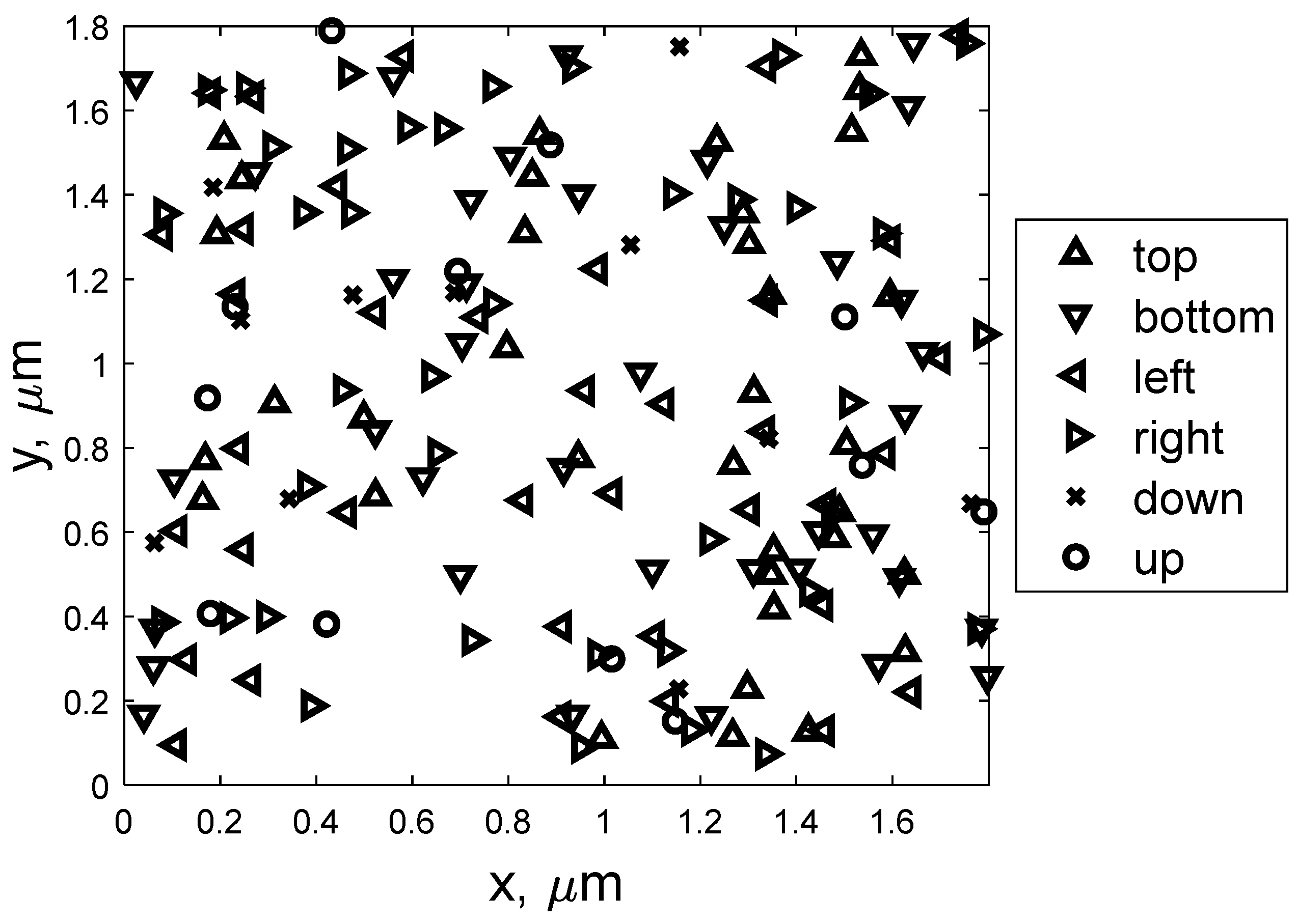
Figure 2.
Number of dislocations versus time during static recovery. Dislocation simulation results are compared with Equation (10). In the figure, the values from Equation (10) are scaled to the same number of initial dislocations.
Figure 2.
Number of dislocations versus time during static recovery. Dislocation simulation results are compared with Equation (10). In the figure, the values from Equation (10) are scaled to the same number of initial dislocations.
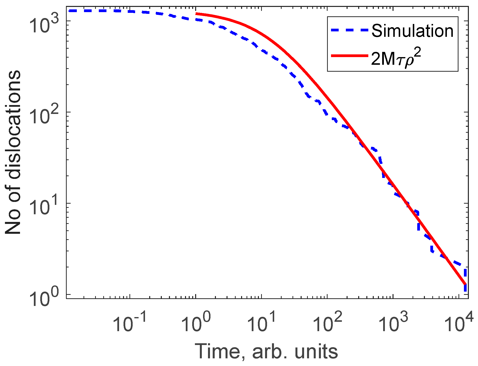
Figure 3.
Stress versus strain for the austenitic stainless steel 17Cr12Ni2Mo0.08C (316H); (a) at room temperature; (b) at 800 °C. Equations (16)–(19) are compared to experimental data from [8].
Figure 3.
Stress versus strain for the austenitic stainless steel 17Cr12Ni2Mo0.08C (316H); (a) at room temperature; (b) at 800 °C. Equations (16)–(19) are compared to experimental data from [8].

Figure 4.
Stress–strain curves in comparison to the extended Equations (20)–(22) for the same data for 316H at room temperature as in Figure 3; (a) room temperature; (b) 800 °C.
Figure 4.
Stress–strain curves in comparison to the extended Equations (20)–(22) for the same data for 316H at room temperature as in Figure 3; (a) room temperature; (b) 800 °C.
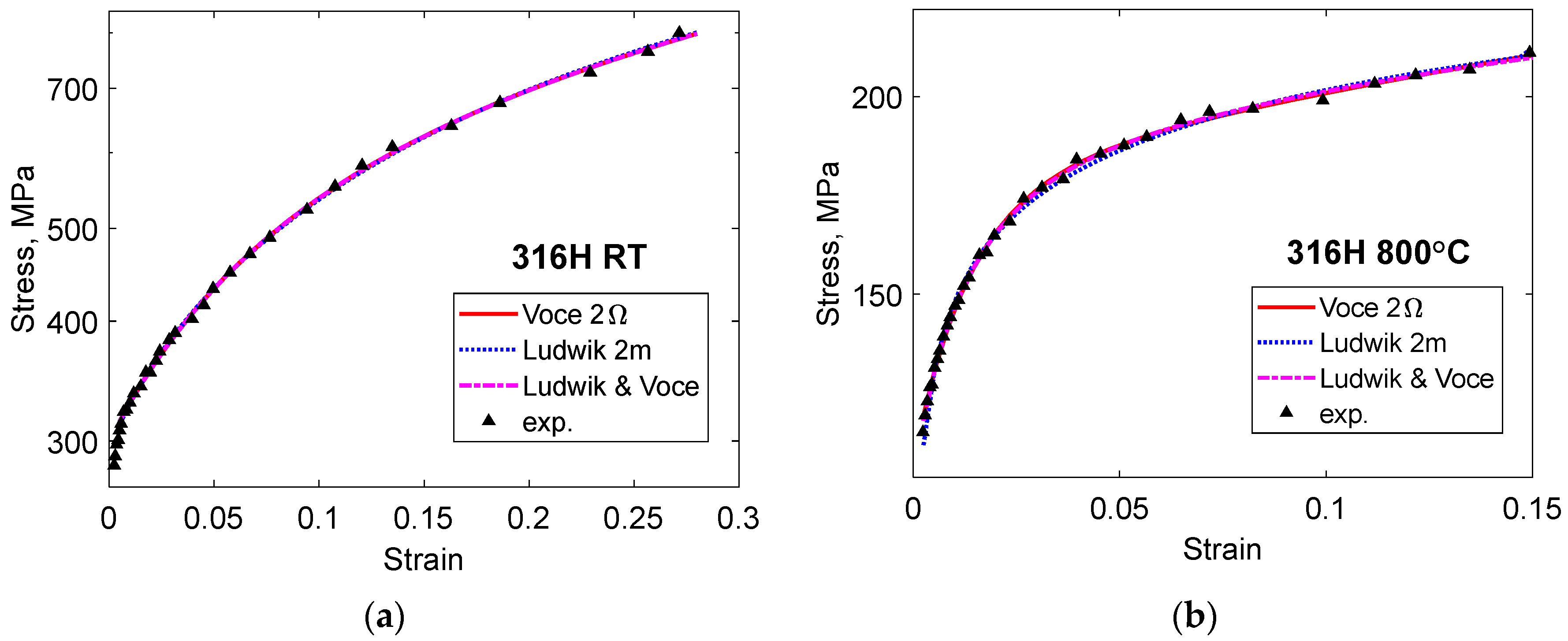
Figure 5.
Stress versus strain for Cu-OFP at 75 °C compared to the model in Equation (25) with experiments. Data from [21]. (a) 1 × 10⁻⁴ 1/s; (b) 1 × 10⁻⁷ 1/s.
Figure 5.
Stress versus strain for Cu-OFP at 75 °C compared to the model in Equation (25) with experiments. Data from [21]. (a) 1 × 10⁻⁴ 1/s; (b) 1 × 10⁻⁷ 1/s.
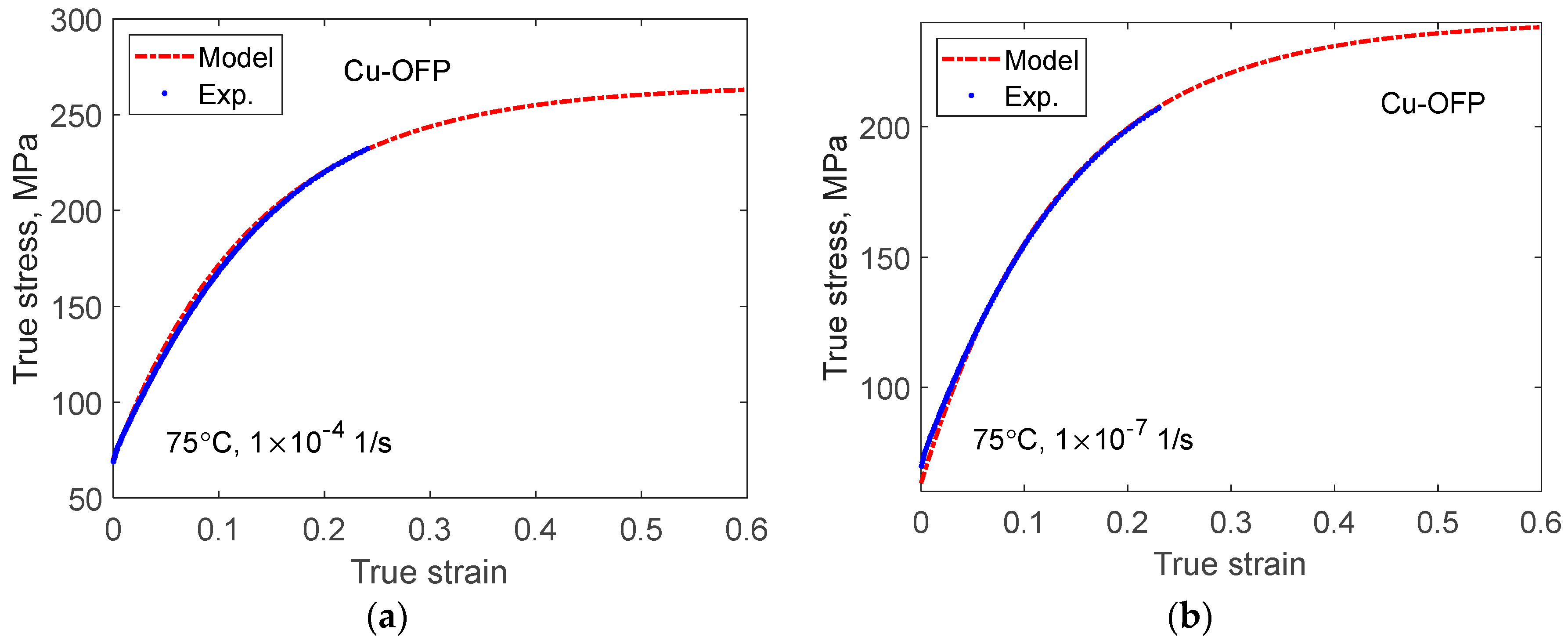
Figure 6.
Stress versus strain for Cu-OFP at 175 °C and 1 × 10⁻⁷ 1/s compared to the model in Equation (25) with experiments [21]. To analyse the role of static recovery (the last term in Equation (14)), results with and without this term are shown.
Figure 6.
Stress versus strain for Cu-OFP at 175 °C and 1 × 10⁻⁷ 1/s compared to the model in Equation (25) with experiments [21]. To analyse the role of static recovery (the last term in Equation (14)), results with and without this term are shown.
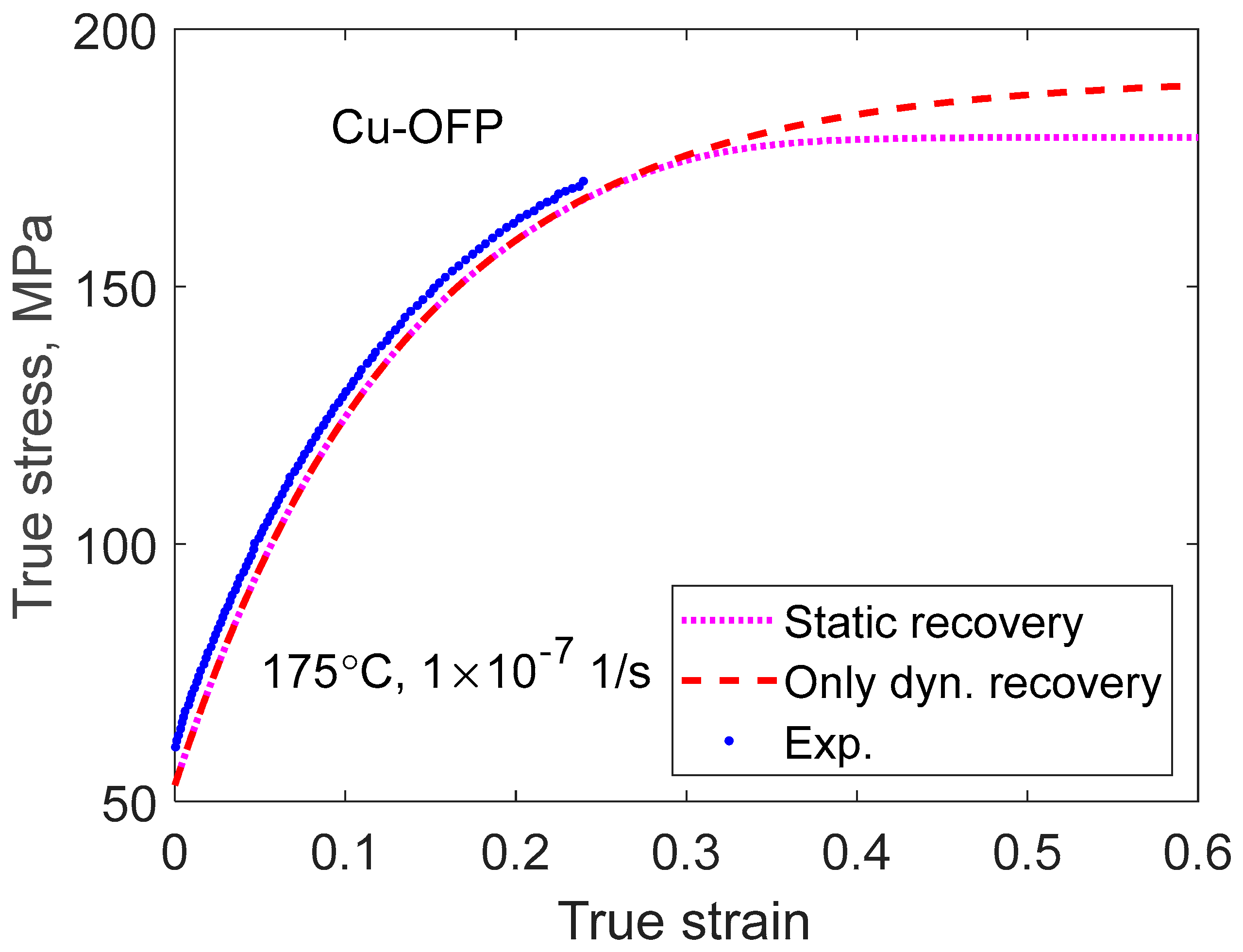
Figure 7.
Secondary creep rate versus stress for pure aluminium. Equation (31) is compared to experimental data from [46]. Reprinted from [7] with the permission of intechopen.

Figure 8.
Secondary creep rate versus temperature at six stresses for pure nickel. Predictions using Equations (31), (34), (36) and (37) are compared to experimental data from [47]. Redrawn from [40] with the permission of ASME.
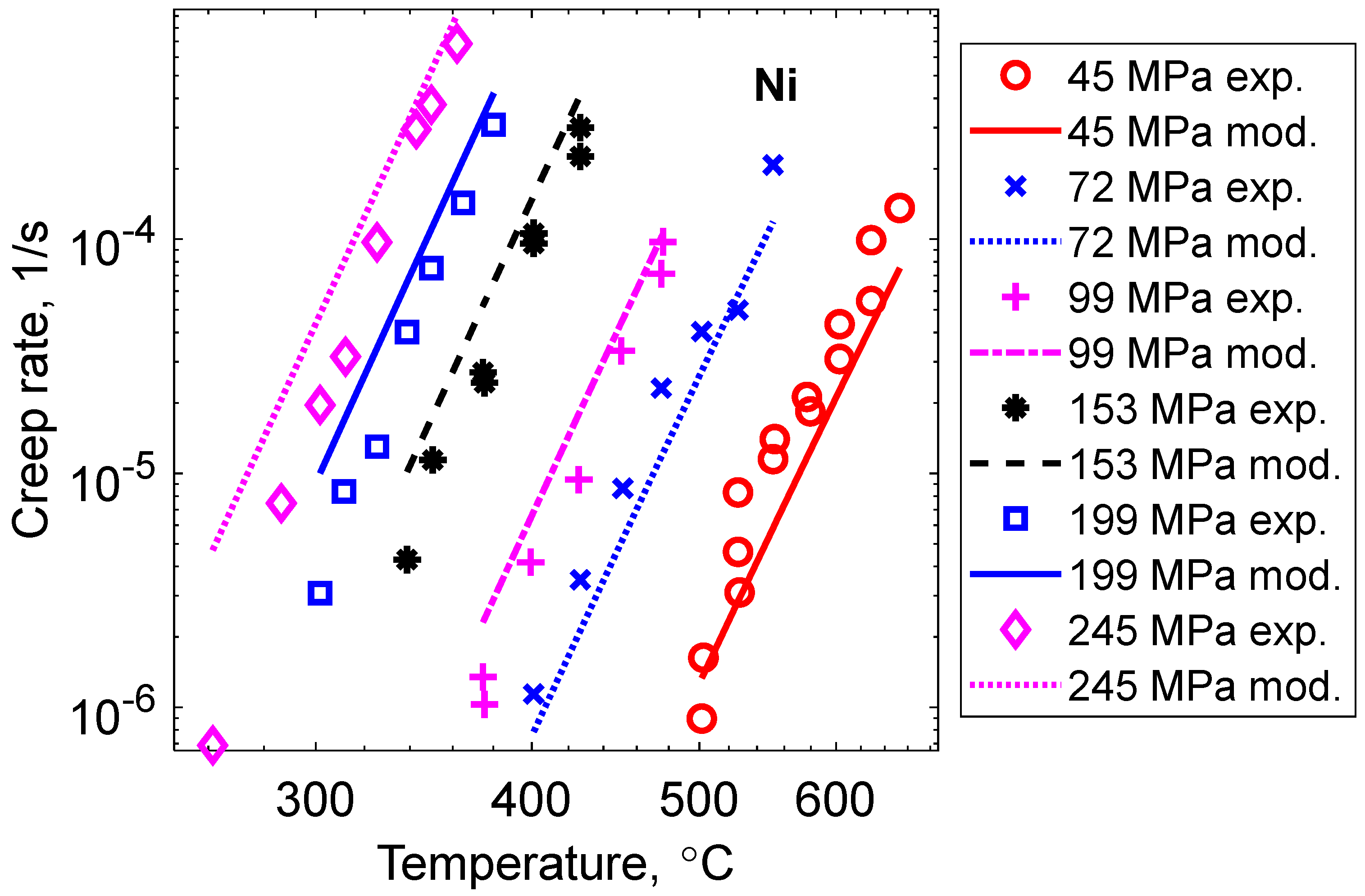
Figure 9.
Creep test of Cu-OFP at 75 °C and 160 MPa. The creep test was interrupted after 12,000 h; (a) creep strain versus time; (b) creep rate versus time, Equation (39). Redrawn from [50] with the permission of Elsevier.
Figure 9.
Creep test of Cu-OFP at 75 °C and 160 MPa. The creep test was interrupted after 12,000 h; (a) creep strain versus time; (b) creep rate versus time, Equation (39). Redrawn from [50] with the permission of Elsevier.
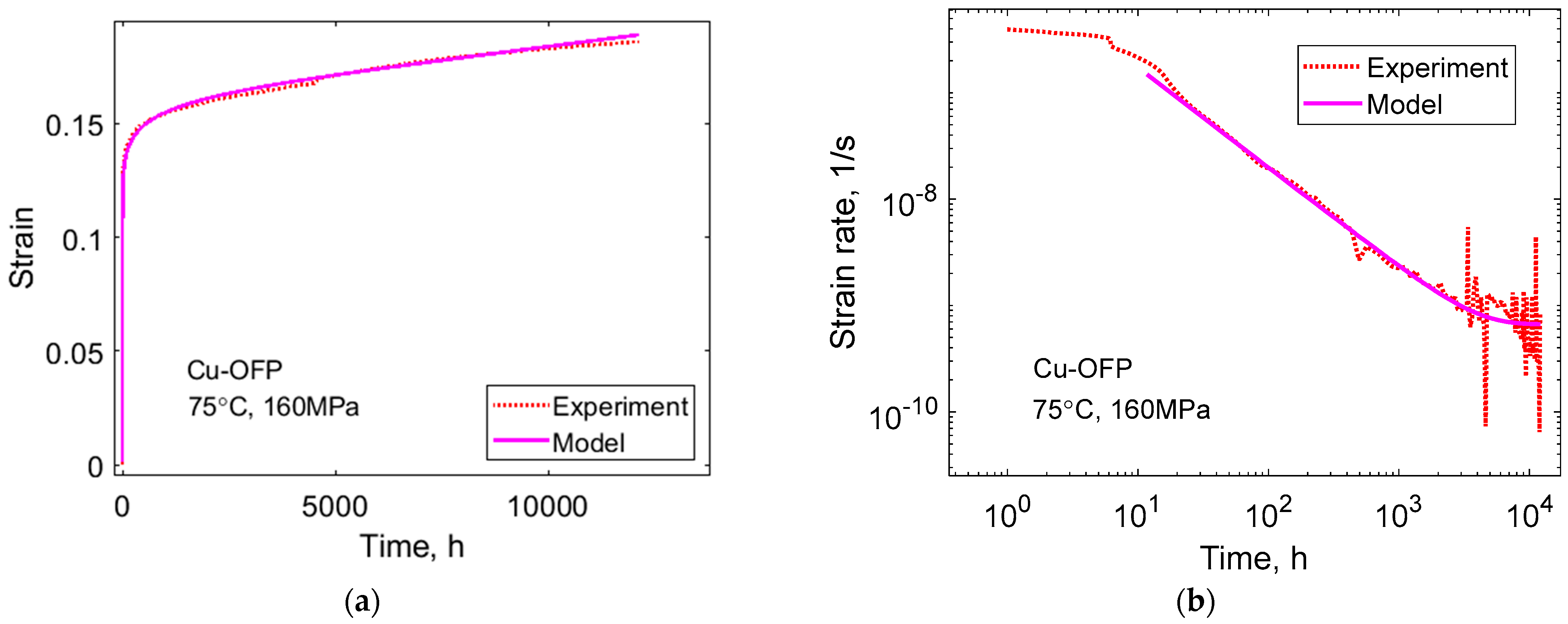
Figure 10.
Primary creep in Cu-OFP at 95 °C, 20 MPa. Experimental data from [53]. Primary creep model in Equation (41). ϕ model according to Equation (45); (a) creep strain versus time; (b) creep strain rate versus time. Reprinted from [49] with the permission of MDPI.
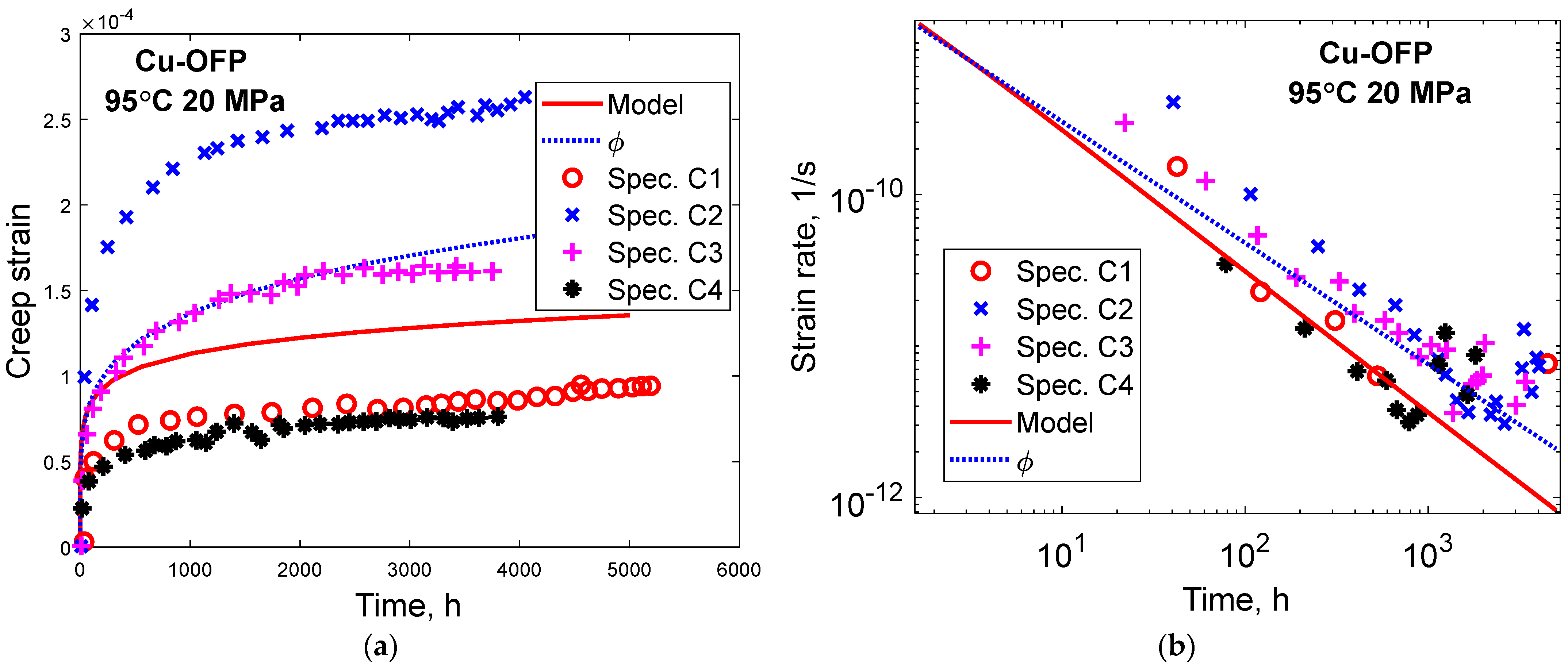
Figure 11.
Creep strain rate versus time for Cu-OFP at 125 °C and 40 MPa for creep rates over extended times. Experimental data from Ho [53]. Reprinted from [33] with the permission of Elsevier.

Figure 12.
Minimum creep strain rates versus stress for Cu-OFP at 600 °C. (a) Experimental data are compared to the model in Equation (31) for Cu-OFP and Cu-OF (without P); (b) experimental data are compared to the classical diffusion creep models for bulk diffusion (Nabarro–Herring creep) and grain boundary diffusion (Coble creep). Reprinted from [33] with the permission of Elsevier.
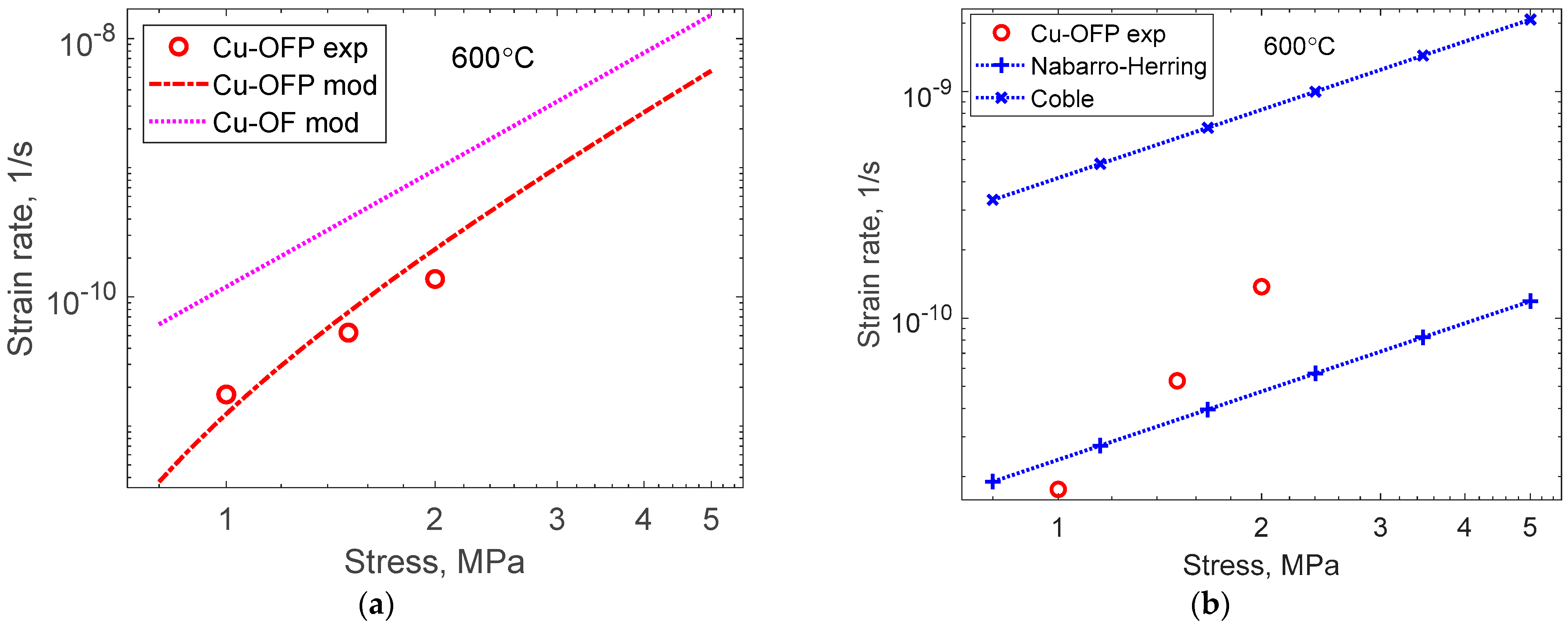
Figure 13.
Creep strain rate versus time at two stresses, 1.5 and 2 MPa, for Cu-OFP at 600 °C. Experimental data are compared to the model in Equation (41). Reprinted from [33] with the permission of Elsevier.
Figure 13.
Creep strain rate versus time at two stresses, 1.5 and 2 MPa, for Cu-OFP at 600 °C. Experimental data are compared to the model in Equation (41). Reprinted from [33] with the permission of Elsevier.
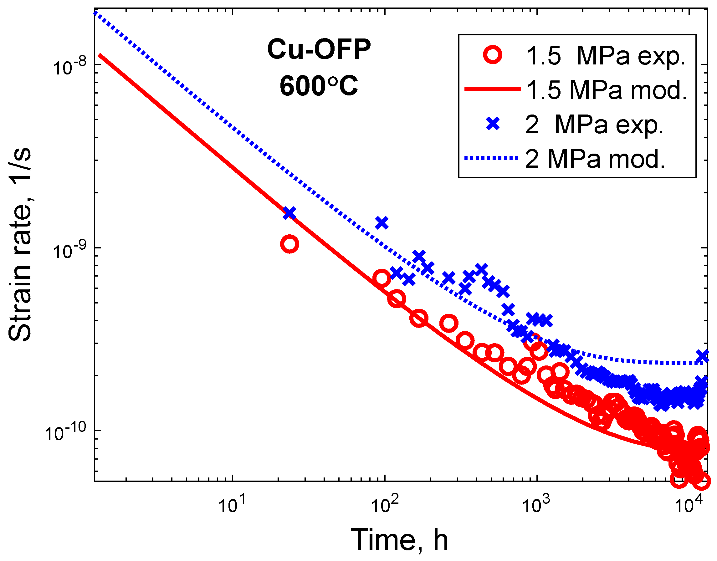
Figure 14.
Creep strain rate versus stress for Al at 650 °C. Experiments are compared to model results. The stationary model is taken from Equation (31) and the primary creep model from Equation (41) after different times. The Nabarro–Herring model for a coarse grain size of 1 mm is also given. Experimental data from [56,58,59,60,61]. Reprinted from [32] with the permission of Elsevier.
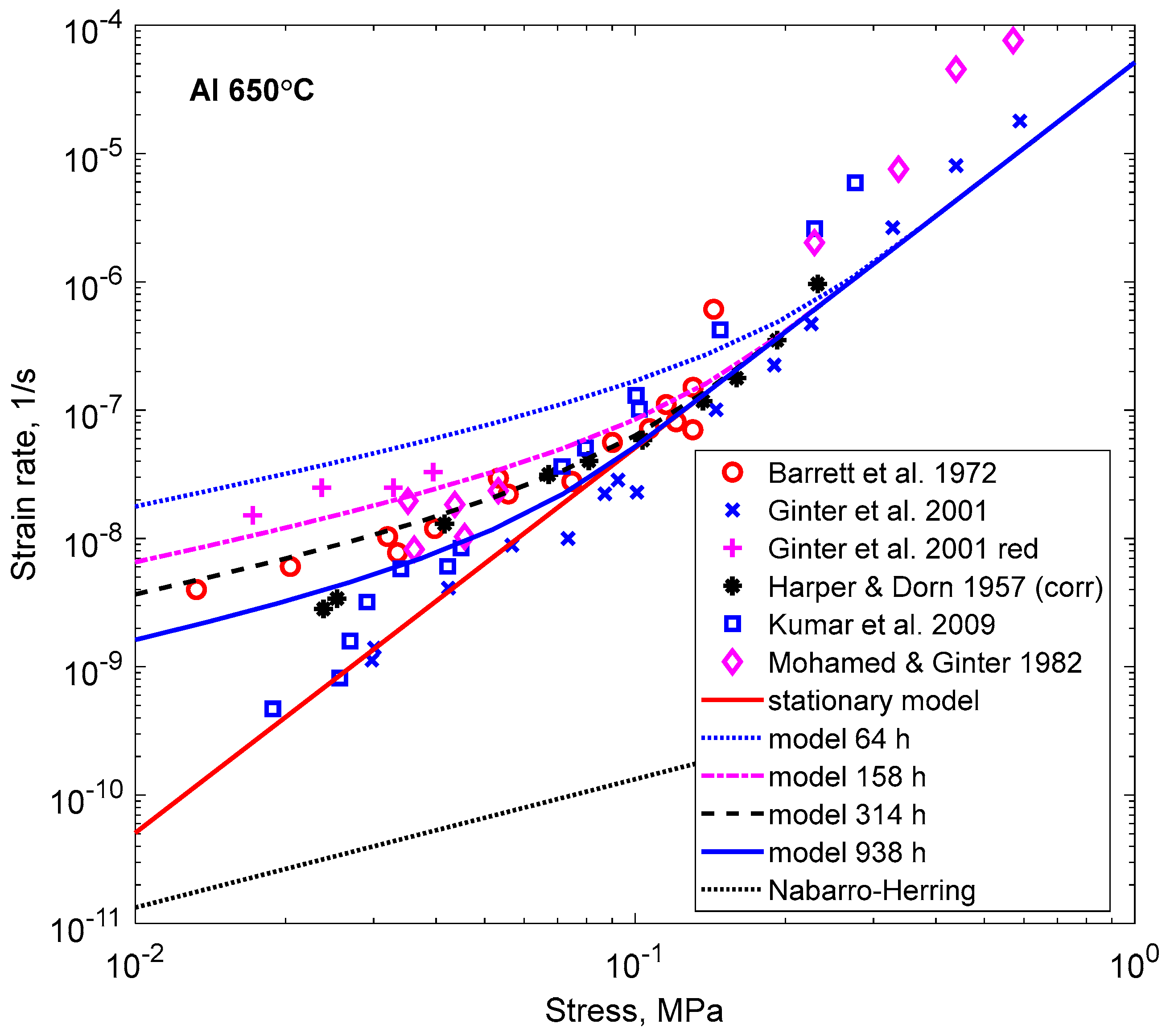
Figure 15.
Creep stress exponent versus stress for Al at 650 °C according to the model in Equation (41) after four times in the primary stage. Reprinted from [32] with the permission of Elsevier.
Figure 15.
Creep stress exponent versus stress for Al at 650 °C according to the model in Equation (41) after four times in the primary stage. Reprinted from [32] with the permission of Elsevier.

Table 1.
Secondary creep rate ratios of copper between 75 and 600 °C.
| Temperature, °C | Stress, MPa | Creep Rate Ratio, Stress | Creep Rate Ratio, Temperature |
|---|---|---|---|
| 75 | 1.5->165 | 4 × 10¹⁸ | |
| 600 | 1.5->165 | 3 × 10¹¹ | |
| 75->600 | 1.5 | 6 × 10¹⁵ | |
| 75->600 | 165 | 4 × 10¹⁰ |
Reproduced from [33] with the permission of Elsevier.
Disclaimer/Publisher’s Note: The statements, opinions and data contained in all publications are solely those of the individual author(s) and contributor(s) and not of MDPI and/or the editor(s). MDPI and/or the editor(s) disclaim responsibility for any injury to people or property resulting from any ideas, methods, instructions or products referred to in the content. |
© 2023 by the author. Licensee MDPI, Basel, Switzerland. This article is an open access article distributed under the terms and conditions of the Creative Commons Attribution (CC BY) license (https://creativecommons.org/licenses/by/4.0/).
Share and Cite
MDPI and ACS Style
Sandström, R. Basic Modelling of General Strength and Creep Properties of Alloys. Crystals 2024, 14, 21. https://doi.org/10.3390/cryst14010021
AMA Style
Sandström R. Basic Modelling of General Strength and Creep Properties of Alloys. Crystals. 2024; 14(1):21. https://doi.org/10.3390/cryst14010021
Chicago/Turabian StyleSandström, Rolf. 2024. "Basic Modelling of General Strength and Creep Properties of Alloys" Crystals 14, no. 1: 21. https://doi.org/10.3390/cryst14010021
Note that from the first issue of 2016, this journal uses article numbers instead of page numbers. See further details here.