FDIP—A Fast Diffraction Image Processing Library for X-ray Crystallography Experiments

Abstract

Serial crystallography (SX) is a cutting-edge technique in structural biology, involving the systematic collection of X-ray diffraction data from numerous randomly oriented microcrystals. To extract comprehensive three-dimensional information about the studied system, SX utilises thousands of measured diffraction patterns. As such, SX takes advantages of the properties of modern X-ray sources, including Free Electron Lasers (FELs) and third and fourth generation synchrotrons, as well as contemporary high-repetition-rate detectors. Efficient analysis of the extensive datasets generated during SX experiments demands fast and effective algorithms. The FDIP library offers meticulously optimised functions tailored for preprocessing data obtained in SX experiments. This encompasses tasks such as background subtraction, identification and masking of parasitic streaks, elimination of unwanted powder diffraction (e.g., from ice or salt crystals), and pinpointing useful Bragg peaks in each diffraction pattern. The library is equipped with a user-friendly graphical interface for facile parameter adjustment tailored to specific datasets. Compatible with popular SX processing software like OnDA, Cheetah, CrystFEL, and Merge3D, the FDIP library enhances the capabilities of these tools for streamlined and precise serial crystallography analyses.

1. Introduction

In recent years, serial crystallography (SX) [1,2] has become an established technique for the determination of protein structures with a particular application in the investigation of small or radiation-sensitive crystals and for the study of fast or irreversible protein dynamics [3,4,5,6]. This has been enabled by the development of new generation X-ray sources such as X-ray Free Electron Lasers (FELs) and the third and fourth generation synchrotron radiation facilities, which produce very bright and coherent X-ray beams, combined with improvements in beamline design and optics, which increase flux density at the sample and thereby decrease the exposure time required to obtain a measurable signal.

Many diffraction patterns are required for the 3D structure determination of a molecule using SX because each crystal is typically exposed only once in a random orientation. Fortunately, the development of modern X-ray detectors made it possible to collect data at an average rate of several kHz [7] so that a full dataset can be acquired in just several minutes [8]. At the same time, such a high data collection rate poses a challenge for data analysis, primarily when used for online feedback. Tools like OnDa [9] offer real-time data analysis of X-ray diffraction experiments, providing investigators with rapid feedback on so-called hit rates [10] and helping them make timely decisions regarding data collection strategies for the current sample. However, the analysis routines must be highly efficient to keep up with the mentioned high data rate.

Before processing the diffraction patterns measured during SX experiments, some pre-processing has to be performed. This includes masking unwanted diffraction and unreliable regions of the diffraction patterns as well as the determination of some features used for further analysis (usually Bragg peaks). Such tasks have to be performed automatically using highly optimised algorithms [11]. Precisely for this reason, the open-source library $FDIP$ was written.

In an SX experiment, the properties of the X-ray source, sample delivery, and detector must all be compatible. Various sample delivery systems have been employed or investigated for delivering micro- to nano-scale crystalline samples into the X-ray beam [12,13]. One class of methods generates a free jet of a liquid suspension of crystals [14,15] that flows continuously across the X-ray beam, and a diffraction pattern is acquired at each X-ray pulse or exposure, whether the beam intersects a crystal or not. A conceptually different approach is to deposit crystals onto a solid supporting membrane, which is then raster scanned in the X-ray beam to collect diffraction in a similarly random fashion [16]. The liquid in the jet, on the substrate or in the crystal, cause radially symmetric background noise. Moreover, the sharp edges of the liquid jets or features on the substrates may produce artefacts in the diffraction image (see Figure 1). The presence of such unwanted diffraction introduces a significant impact on data analysis, necessitating meticulous attention and corrective measures.

Other artefacts, such as ice or salt rings (see the left plot in Figure 2), can also significantly affect the final result of data processing. Conventional crystallography usually excludes these artefacts by omitting the whole resolution ranges where the rings are observed. However, the advantage of serial crystallography is that such artefacts may not be present in every recorded diffraction pattern. So, the resolution ranges containing rings must be excluded only for the patterns where the rings are detected and not for the patterns without observable ice and salt diffraction. Thus, in the case of SX, the final dataset can be complete and not influenced by the rings’ artefact.

The initial step of indexing measured diffraction patterns involves precisely determining the positions of the Bragg peaks. Many peak-finding algorithms rely on discerning these peaks from the background, often leveraging the inherent radial symmetry to estimate background levels. This approach is exemplified in the $peakfinder8$ algorithm, as implemented in Cheetah [10]. However, challenges arise when radial symmetry is disrupted, as seen in scenarios such as the presence of shadows or an asymmetrical attenuator, as illustrated in Figure 3. In such cases, a local background estimation becomes advantageous, and this strategy is integrated into the $peakfinder9$ algorithm, a component of the FDIP library.

Peaks in the diffraction pattern not only originate from the crystal but many diffraction artefacts, such as the streak from the jet (see Figure 4), may contain or resemble peaks or rings (see Figure 2). To exclude these peaks from the crystal diffraction analysis, the region of the artefacts has to be excluded from the peak search area by masking. This can be performed automatically with the $streakFinder$ and $ringFinder$ algorithms. Both algorithms rely on calculation of the radial profile for every diffraction pattern. That is why an efficient algorithm for calculating the radial profile of a pattern was developed. The developed algorithm takes special care to handle circles with small radii, containing only a few pixels.

Different functions of the $FDIP$ have multiple parameters to tune for each collected SX dataset. To adjust the parameters, a GUI was developed named $FDIP\_tweaker$. This GUI allows a user to load a set of patterns and, while modifying different parameters, observe the performance of each applied filter in real time or as the results of the peak finding.

2. Materials and Methods

2.1. Handling a Bad Pixel Mask

X-ray detectors commonly exhibit non-functional pixels called bad pixels. Additionally, parasitic diffraction regions frequently arise, necessitating their exclusion from the analysis. These designated areas are delineated within a mask, conventionally stored as an array where each element corresponds to an individual pixel.

The good practice is to store the mask in the files according to community-accepted metadata standards [17,18]. But internally, every software package can treat the mask differently. Various software tools, such as Cheetah [10] and OnDA [9], utilise arrays of bytes, while CrystFEL software [19] employs arrays of integers. Since elements from the mask array are frequently accessed, optimising access efficiency is paramount. To achieve this, we adopt a strategy of embedding the mask directly into the data by changing the intensity of the pixels that have to be masked by some special value. This conserves memory loads and minimises cache space usage, decreasing execution time.

Additionally, we explore the option of saving the mask as a sparse array, especially suitable for masks with a small number of masked pixels. In this scenario, only the coordinates of the masked pixels are stored, potentially accelerating the merging process.

2.2. Algorithm Descriptions

The following functions and programs of FDIP are described in detail:

• Radial background subtraction—a set of functions used to calculate radial background for further subtraction on the pattern-by-pattern basis.
• $StreakFinder$—an algorithm to mask the radial streaks at the diffraction patterns.
• $RingFinder$—an algorithm to mask the sharp rings at the diffraction patterns. It also works with just a set of strong Bragg peaks at a single radius (not just uninterrupted rings).
• $peakfinder9$—an algorithm to find Bragg peaks in diffraction patterns, that is, using local background estimation to determine the peaks’ location.
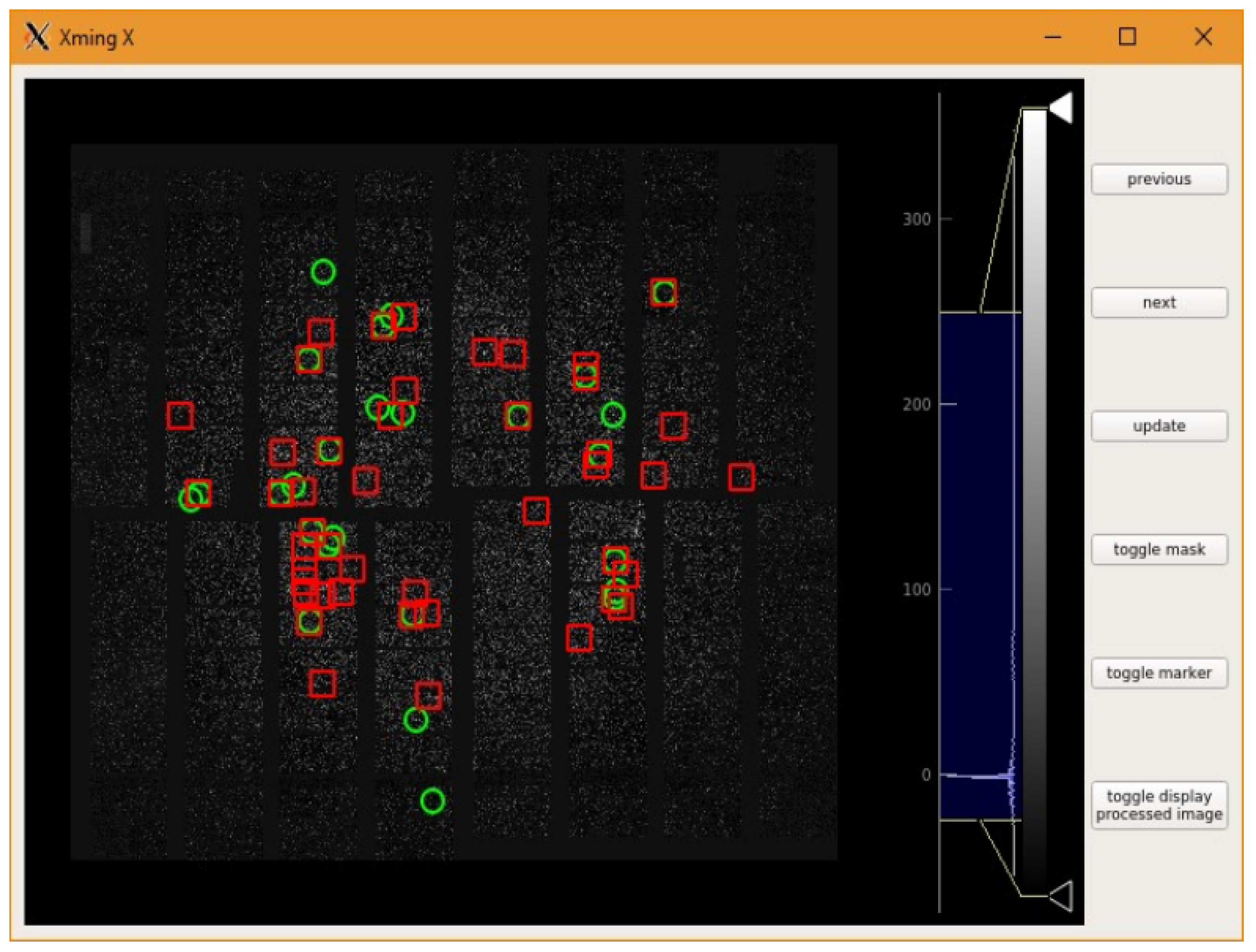
• $FDIP\_tweaker$—a GUI that can be used for the optimisation of parameters for all the algorithms mentioned above.

2.2.1. Radial Background Subtraction

The background in diffraction patterns typically arises from the scattering of X-rays by air or the sample’s supporting medium. Consequently, this background is generally characterised by radial symmetry (after applying polarisation correction and taking care of the shadows). Estimating and subtracting the radial background from the data per image for subsequent analysis is often needed. All the radial background estimation functions described here rely on the good knowledge of the detector geometry [20].

The crux of radial background subtraction lies in accurately estimating the background, denoted as $I\left(r\right)$, where r represents the radius. One straightforward approach involves dividing the radius into equally sized bins and calculating an average value for each bin. This approach has one obvious drawback: bins close to the centre of the diffraction pattern (the position of the direct beam at the detector) contain just a few pixels. Therefore, the error in estimating the average value might be high. One approach to overcome this issue is pixel splitting, used in pyFAI [21], where the geometrical size of the pixel is used to distribute the value of each pixel to different radial bins. We use a different approach to address this issue: dynamically sized bins. The selection of bin sizes is critical: each bin must encompass enough values to ensure a robust statistical estimate while covering a minimum radius range. This approach is computationally efficient and works well for the data where the background changes slowly with the radius (typical for SX).

We introduce the parameters minValuesPerBin and minBinWidth to achieve a suitable distribution. Starting from the closest pixel to the centre, the dynamic bin width is set to the smallest possible value, limited by minBinWidth. The bin contains a minimum of minValuesPerBin pixels. To enhance the performance, not every pixel within a bin contributes to the statistical estimation. If a bin surpasses the limit defined by maxConsideredValuesPerBin, only maxConsideredValuesPerBin evenly distributed pixels are considered. The bins and their associated pixels are pre-computed at program startup. These modifications of the standard radial average calculation considerably speed up the calculation.

Following the allocation of data to the bins, the kth order statistic, representing the kth smallest value within each bin, is computed. The parameter rank defines k on a scale from 0 to 1, proportional to the range from 0 to the number of considered values in the bin. For instance, setting rank = 0.5 calculates the median, while rank = 0 and rank = 1 yield the minimum and maximum values, respectively. This flexibility is crucial because opting for the median might be inappropriate in scenarios dominated by extremely high or low values, as exemplified in Figure 5 where streaks are prevalent.

In evaluating $I\left(r\right)$, the values within the bins undergo linear interpolation or extrapolation. Subsequently, the background subtraction entails assessing $I\left(r\right)$ at the corresponding radius for each pixel and deducting this value from the pixel intensity.

2.2.2. Streak Masking

Streaks are defined as artefacts pointing in the radial direction having an overall decreasing intensity with the increasing radius. Streaks are generally very noisy, so the intensity decrease is not monotonic. Figure 1 shows sample diffraction patterns with a streak artefact.

The $StreakFinder$ algorithm searches for streak-like features near the detector centre, using the pre-set of pixels defined by streakStartPixelCandidates (usually pixels close to the centre of detector). After a streak is identified, it is traced to its end in a radially increasing direction. Having found the streak’s end, all pixels along the streak (lying in a radial direction between the beam centre and the streak end) are masked.

To identify the streak a custom non-linear filter is applied, which amplifies the streak pixels and suppresses the rest, in particular, the Bragg peaks—see Figure 6a,b. This filter works in the following way: lines of pixels in the radial direction are replaced by the average of the pixels’ intensity values, which are smaller than the median of all intensity values of that line. In this way, the filter gets rid of all Bragg peaks with the size smaller than the half length of the lines. At the same time the streaks are preserved if they have a length comparable to that of the lines—Figure 6b. The filter is parameterised via the parameters filterLength and filterStep, where filterLength defines how many pixels will be taken into account for every filter value and filterStep defines how far the pixels are separated from each other. The line segment’s length can be computed as (filterLength − 1) * filterStep.

The application of the filter is very computationally expensive. Thus, instead of applying the filter to the entire detector, a lazy estimation scheme is used, i.e., a filtered value is calculated only when requested. To further boost the execution speed, all positions of the pixels (the lines) needed to compute the filtered values are pre-computed at program startup.

Finding the end of a streak is not trivial since the intensities of the pixels along the streak tend to fluctuate, especially at the end of the streak (see Figure 4). This is solved by adding inertia to the streak tracing. Only when hitting several consecutive non-streak pixels, the end of a streak is defined. The exact number of consecutive non-streak pixels are defined in the parameter streakElongationMinStepsCount and a number proportional to the radius. The latter is parameterised via streakElongationRadiusFactor. Such an approach is justified by the fact that long streaks fluctuate significantly more than short ones.

To estimate the statistics of the background signal, the pixels that do not belong to the streaks are used. To find such pixels, knowledge about the streak location is needed. Typically, at one diffraction pattern, the streaks are oriented in only one direction. Defining several rectangular regions evenly distributed at a radius where streaks usually occur has the effect that some of these regions will be located in a streak-free environment with a sufficiently high probability. The parameter backgroundEstimationRegions defines the rectangular background estimation regions. Due to the increased likelihood of a region being hit by a streak, the statistics from the region with the second smallest mean are taken as the actual background estimation. A pixel is recognised as a streak pixel if the filter outcome is sigmaFactor times the standard deviation higher than the mean of the background.

After a found streak is masked, all the neighbouring pixels are also masked. The size of the additionally masked region is defined by the parameter streakPixelMaskRadius. Figure 6c shows an example of masked streaks. All pixels that must be masked for each possible streak end are pre-computed at program startup to reduce this time.

The $streakFinder$ algorithm has been successfully used in [22] as well as for many other beamtimes, especially aimed for merging the measured intensities into the 3D reciprocal space [23,24].

2.2.3. Ring Masking

Ring artefacts do not always cover all angles but can have a predominant angle range (see the left plot in Figure 2). A ring artefact usually appears due to undesired diffraction from some crystalline powder (ice, salt, concentrated SX sample, etc.)—a so-called Debye–Scherrer ring. Such a ring is generally several pixels wide and contains pixels with high values. The radial average, computed with a bin width of 1 pixel, is employed to identify ring artefacts. Although utilising the kth order statistic might yield superior results at this stage, we have opted for the radial average due to its significantly lower computational cost than the kth order statistic. Post-processing operations are applied to address noise in the radial average. These operations are specifically designed for radial bins, making them computationally inexpensive.

The idea behind the ring masking is that significantly well-observable rings will be present in a graph of radial averages as rather sharp peaks. These peaks are identified by comparing the actual radial averages with a version smoothed by a median filter. This method will also work if the observable parasitic diffraction does not form uninterrupted rings but is present in several large diffraction spots observed at the same radius.

The first operation applied to the radial bins is a median filter with a length defined by the parameter smoothWindowRadius—this operation produces a smooth radial curve. The median filtered bins m are subtracted from the actual radial bins b and normalised by b, leading to the relative difference $d=\frac{b-m}{b}$. For further noise reduction, $d^{\prime }$ is constructed from d by filtering it with a median filter of width 3. This excludes cases where a strong Bragg peak at low Q (close to the direct beam position at the detector) can significantly influence the radial average. Bins in $d^{\prime }$ exceeding the parameter relaltiveRingDiff are marked as ring radii. Since rings can have smooth borders, the program allows for the widening of the found rings by the parameter ringDilationRadius. The parameters minRingRadius and maxRingRadius define the the radial shell over which to search for rings.

2.2.4. Peak Finding

Bragg peaks manifest as relatively small, high-intensity regions on the detector, often characterised by a Gaussian-shaped intensity profile. The diameter of a Bragg peak can vary based on the experiment setup and crystal size, ranging from as small as one pixel to significantly larger, spanning 16 or more connected pixels. A standard and efficient method for identifying Bragg peaks in diffraction image analysis involves signal and background estimation. This method identifies a peak if the signal-to-noise ratio surpasses a specified threshold. Notably, this approach has demonstrated speed and utility, being employed in programs like Cheetah [10], CrystFEL [19], OnDA [9], and XDS [25]. Hence, we adopt this established approach, emphasising the combination of robust signal and background estimation to achieve minimal execution times.

A straightforward approach to background estimation involves defining constant background statistics. While this method is the quickest, it may fall short in scenarios where backgrounds vary. In SX diffraction images, the background often exhibits radial symmetry, making it meaningful to estimate the background statistics depending on the radius. This fast method can provide excellent statistics since many data points are available to estimate every value. Notably, the widely used $peakfinder8$ algorithm in Cheetah software adopts this radial approach [10].

Alternatively, a local background estimation can yield superior results for diffraction images lacking a radially symmetric background. Radial symmetry may be disrupted by diverse characteristics in different detector panels, parasitic shadows from various beamline components or the sample holder, other sources of parasitic scattering, or a special experimental design that disrupts the radial symmetry. An example of the latter is using an off-centred attenuator, as illustrated in Figure 3.

While local background estimation might be computationally intensive, it is the most versatile method. In the case of the $peakfinder9$ algorithm, we chose the local, instead of radial, background estimation to avoid issues due to the shadows and unwanted diffraction.

The fundamental concept behind the $peakfinder9$ algorithm remains consistent with that of $peakfinder8$. Noise is presumed as uncorrelated and Gaussian distributed, allowing for a straightforward description of a confidence interval using the mean and standard deviation. Notable distinctions from $peakfinder8$ include advancements in local background estimation and additional options for fine adjustment.

Whether a pixel is considered as a peak pixel relies on analysing its local square-shaped neighbourhood, as defined by the parameter windowRadius. This neighbourhood is subdivided into three distinct regions: the direct eight neighbours of the pixel, the border pixels, and the remaining interior pixels (refer to Figure 7 for a visual representation).

Each pixel is subjected to a series of filter conditions designed to filter out most non-peak pixels in the initial stages with minimal computational effort:

• $I_{x,y}>I_{Border}+c_1$
• $I_{x,y}>I_{x\pm 1,y\pm 1}$
• $I_{x,y}>\mu +c_2·\sigma$
• ${\sum }_{I_{a,b}>\mu +c_3·\sigma }{I}_{a,b}>\mu +c_4·\sigma$

Here, $I_{x,y}$ stands for the intensity of the pixel at position $(x/y)$, $\mu$ and $\sigma$ are the mean and standard deviation of the border pixels, and $c_1$ to $c_4$ are constants for the adjustment of the accuracy of the algorithm.

The first condition trades speed for accuracy. Peak pixels should have higher intensity than non-peak pixels. $c_1$ sets a constant offset that the peak pixel has to surpass each border pixel to be recognised as a peak pixel. $c_1$ is defined by minimumPeakOversizeOverNeighbours. For performance reasons, the implementation does not check all border pixels, but only three on each side of the border, i.e., 12 in total. The checking process is structured to prioritise the pixels most likely present in the cache memory, ensuring that they are examined first to minimise the overall memory load.

The second condition ensures that the pixel has higher intensity compared to its direct neighbours. This way, only the most intense pixel of a peak passes the condition. Without this condition, multiple pixels of a peak could be identified as valid peaks, and there would be a need for an additional step that selects the largest of the pixels as the peak centre.

The third condition, shared with $peakfinder8$, assumes a Gaussian distribution, establishing a confidence interval based on statistics estimated from the border pixels. The parameter sigmaFactorBiggestPixel defines the threshold $c_2$.

For the last condition, the peak is integrated by summing up all pixels within the region in the confidence interval defined by $c_3$, i.e., the ones that are big enough to count as peak pixels. Only integrated peaks that are strong enough to be in the confidence interval of $c_4$ pass the last condition. A meaningful setting of the constants can be constrained by $c_3\le c_2\le c_4$. This way, weak pixels belonging to a peak are respected while still robust to noise. For even more robustness, only connected pixels are respected. The parameters defining $c_3$ and $c_4$ are sigmaFactorPeakPixel and sigmaFactorWholePeak, respectively.

A visualisation of the three parameters of $c_2$ to $c_4$ can be found in Figure 7.

2.3. Parameter Tweaker

Tweaking parameters of the described functions for different datasets can be cumbersome if the user does not have a tool for fast feedback. We created the graphical user interface (GUI) for tweaking parameters (visit the repository of $FDIP\_tweaker$ https://gitlab.desy.de/oleksandr.yefanov/fdip_tweaker, accessed on 31 January 2024). It is a Python-based GUI that uses C++ code of the FDIP library.

The $FDIP\_tweaker$ executes the algorithms in the following order:

• $peakfinder8$;
• $ringFinder$;
• $radialBackgroundSubtraction$;
• $streakFinder$;
• $peakfinder9$

The GUI of the $FDIP\_tweaker$ is presented in Figure 8. The execution parameters are specified in an $accuracyConstants.ini$ file. Only algorithms defined in the $.ini$ file are executed and applied to the loaded diffraction image.

The graphical user interface (GUI) facilitates the navigation through images within a dataset, displaying mask and image data and the identified peaks from the $peakfinder8$ and $peakfinder9$ algorithms. An update button within the GUI allows users to seamlessly modify parameters in the $accuracyConstants.ini$ file without exiting the interface.

3. Results

The core concept behind the FDIP library was to create functions tailored for efficient and reliable processing of serial crystallography (SX) data. These functions were developed to meet the challenges and address specific tasks observed during SX experiments conducted at various facilities. Each function underwent rigorous testing with real datasets to ensure robust performance across diverse scenarios.

This chapter presents the outcomes of applying the developed functions to real data, showcasing their effectiveness. Additionally, selected FDIP functions are compared with analogous functions from other packages, such as the comparison between $peakfinder9$ from FDIP and $peakfinder8$ from Cheetah.

3.1. Execution Time Measurement

All execution time measurements are conducted on a CPU with an E5-2640 v3 processor operating at a clock speed of 2.60 GHz. It is important to note that the data is presumed to be loaded and fully pre-processed to enable the algorithm to execute. While all the algorithms presented here were optimised to minimise adverse effects on concurrently executed threads, the evaluation focuses explicitly on single-thread performance. This choice is deliberate to avoid the impact by the parallel execution of different algorithms.

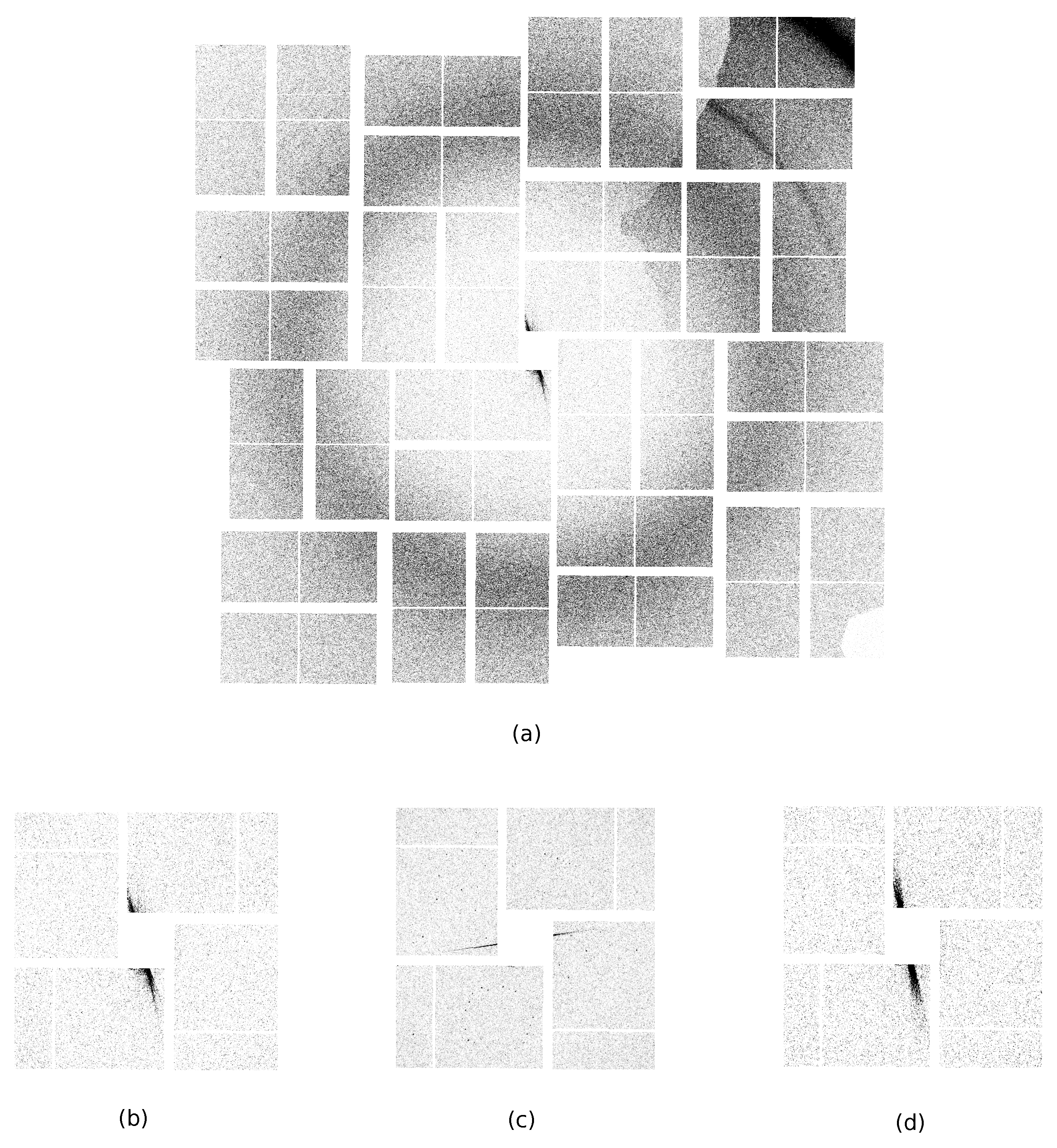
3.2. Radial Background Subtraction

To assess the effectiveness of the radial background subtraction algorithm presented in this study, we conduct a comparative analysis against the widely adopted radial background subtraction algorithm found in the Cheetah software [10]. We focus the evaluation on the most critical parts of the radial background subtraction: parts of the image with few pixels available for statistics estimation, streak artefacts, and execution time.

We compared the background subtraction function in our provided method (FDIP) and the corresponding function utilised in Cheetah. This evaluation was performed on two datasets, each comprising 2000 patterns, captured with different detector sizes: PILATUS 6M (collected during SARS-CoV-2 research at the P11 beamline of the Petra III synchrotron in 2020 [26]) and Eiger 16M (from unpublished research at P14 in 2019). As depicted in

Table 1. The speed comparison of background subtraction functions in FDIP (Fast Diffraction Image Processing) and Cheetah [10].

	Eiger 16M	PILATUS 6M
FDIP	0.05 s	0.02 s
Cheetah	4.96 s	1.63 s

, the key finding is that the FDIP background subtraction function is approximately 80 times faster than Cheetah for the 6M detector size. For the 16M detector size, it is about 99 times faster. This improvement is due to the pre-calculation of the radial bins and their corresponding sparse selection of contributing pixels, which has to be performed once for all diffraction patterns. It takes about 1 s for Pilatus 6M and almost 4 s for the Eiger 16M.

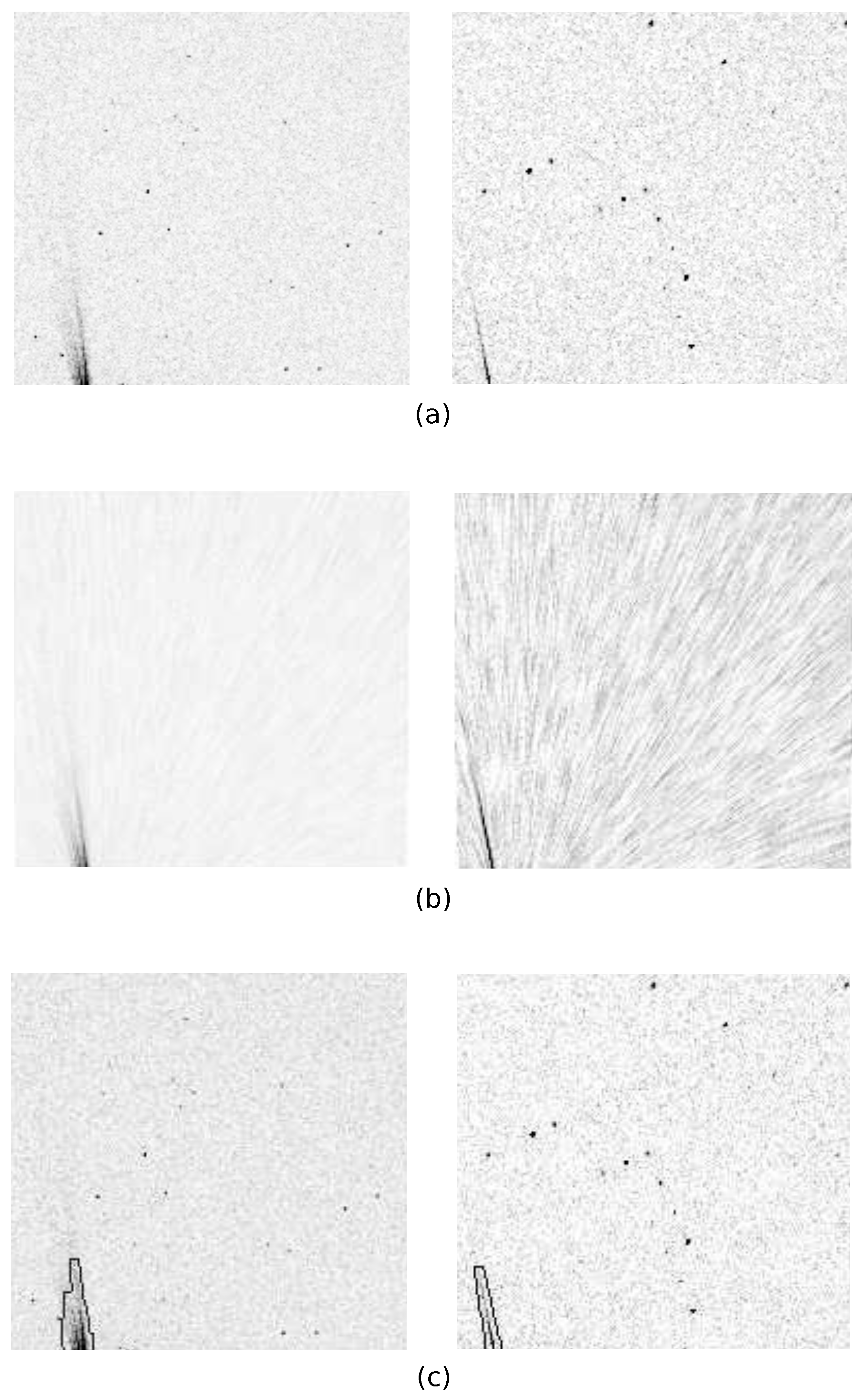
3.3. Streak Masking

The pre-computation time required for the efficient execution of the $streakFinder$ is notably influenced by the detector size and the parameter streakStartPixelCandidates. For the CSPAD detector [27], this pre-computation typically takes around 4 s. However, the pre-computation time can extend to 1 min or more for detectors featuring larger ASICs.

The execution time of the streak finder is predominantly contingent on the presence of a streak. On the CSPAD detector [27], in the absence of a streak, the execution time is less than one millisecond. For patterns containing small streaks, the execution time ranges from 1 to 2 ms, while for larger streaks, it reaches approximately five milliseconds. In setups where a streak can cover half of the detector, the execution time may be higher. Despite its inherent complexity, it is noteworthy that the streak-finding algorithm constitutes an insignificant portion of the overall execution time in the entire data processing pipeline.

To assess the performance of the $streakFinder$ algorithm, we utilised a dataset from an experiment conducted at the Atomic Molecular and Optical (AMO) beamline at LCLS in 2016. The liquid jet was used as a sample delivery method, generating streaks of high intensity when the beam hit the wall of the jet. The dataset was measured with pnCCD detectors, capturing soft X-rays and exhibiting extensive streaks. Visual comparisons of patterns before and after applying the $streakFinder$ algorithm are presented in Figure 5.

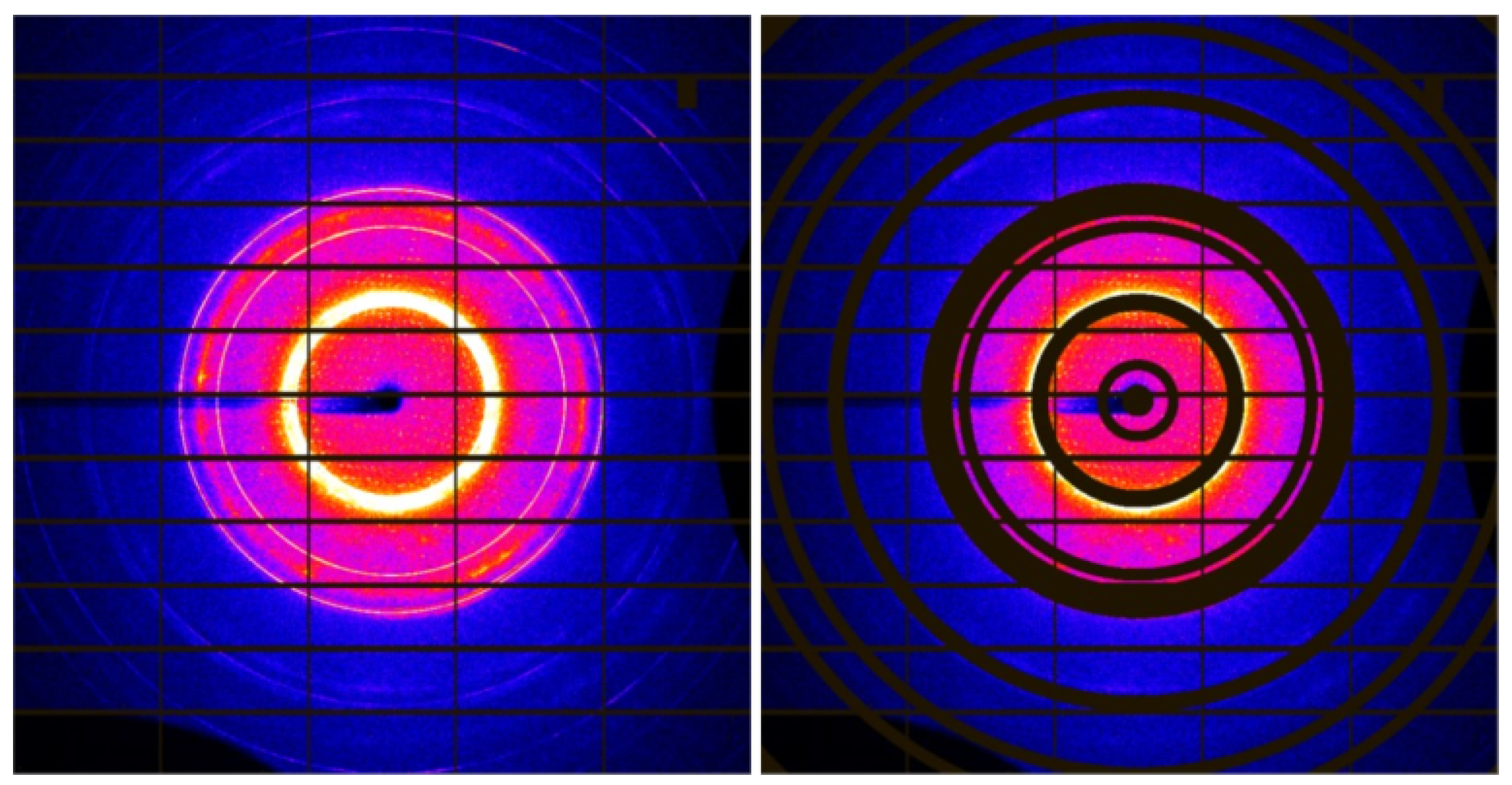
3.4. Ring Masking

The $ringFinder$ algorithm underwent testing on datasets for two samples, each comprising 2000 patterns, collected during SARS-CoV-2 research at the P11 beamline, PETRA III [28], with a Pilatus 6M detector (refer to Figure 2). The evaluation involved visual comparisons and calculations of such figures of merits for data quality assessment as $C{C}^{*}$ and $R_{split}$, respectively (see Figure 9)—the way how those metrics are calculated can be found in [19,29,30]. $C{C}^{*}$ ranges from 0 to 1, with values closer to 1 indicating a better fit between the observed and calculated structure factors. $R_{split}$ is an analogue of $R_{merge}$, used in conventional crystallography: a lower $R_{split}$ value indicates better agreement between two halves of the datasets, and thus, higher precision.

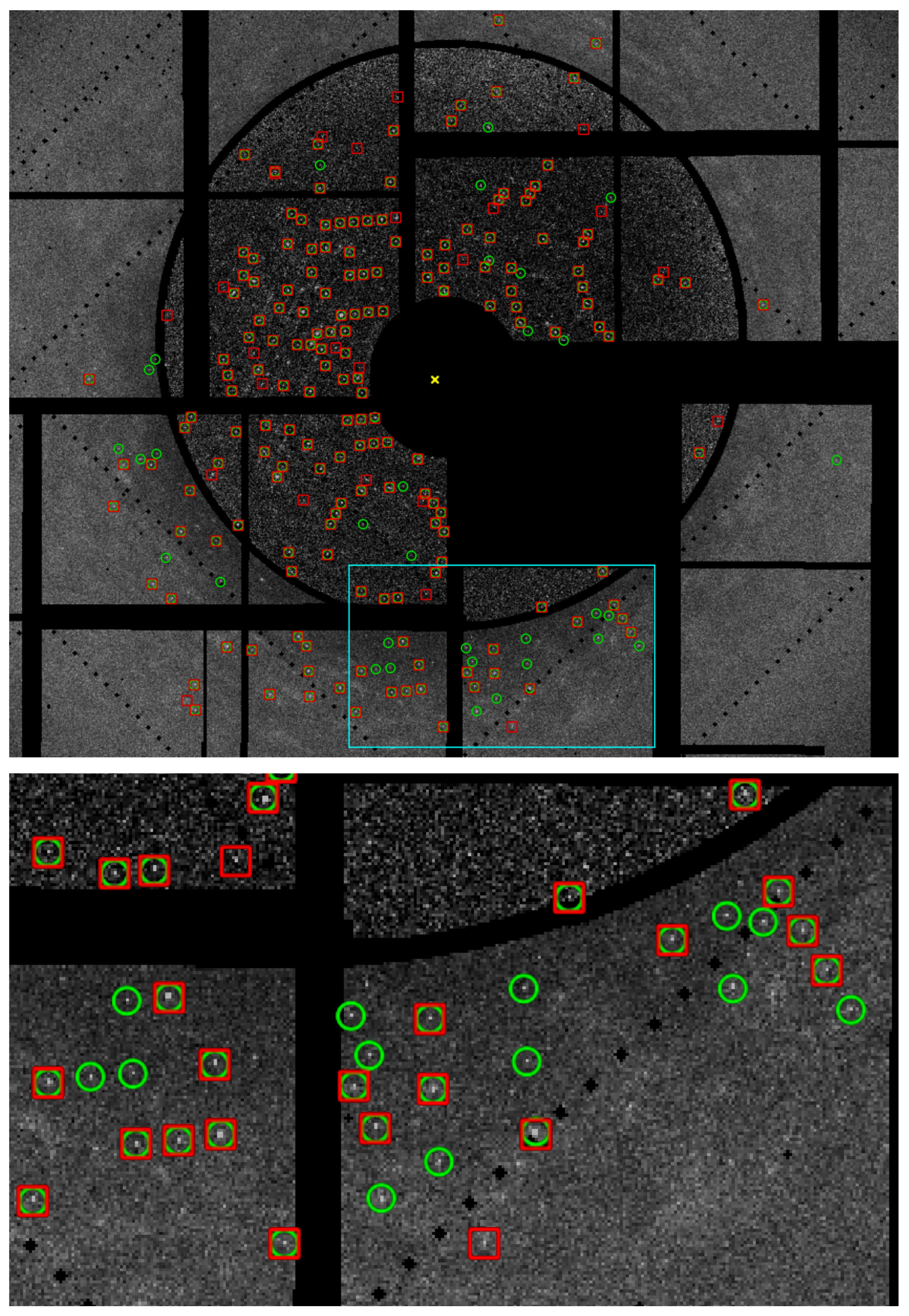
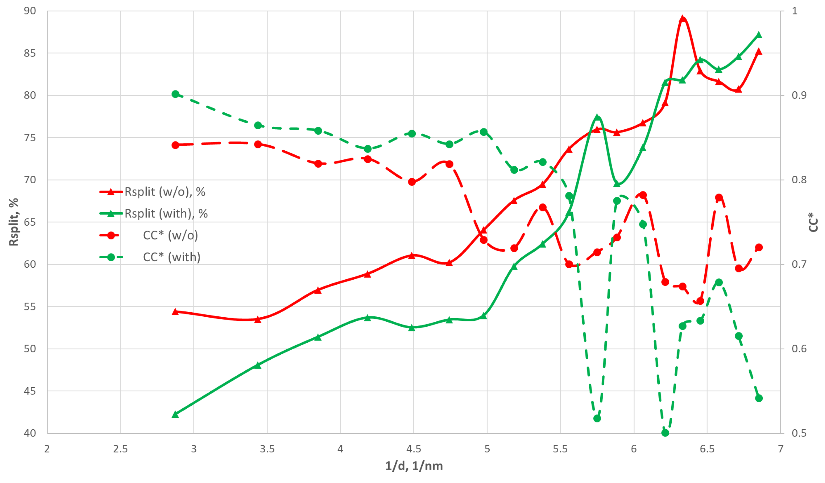
3.5. Peak Finding

The $peakfinder9$ algorithm is based on the widely used $peakfinder8$ algorithm. The differences are the local background estimation in $peakfinder9$ instead of the radial background used in $peakfinder8$. This makes the algorithm more robust to different obstacles often observed in diffraction patterns. Since the evaluation of the peak finding of weak peaks (i.e., border cases, where the option of having a more flexible threshold gives a benefit) is hard to quantify and relies heavily on parameter tweaking, we focus the evaluation on the local background estimation and the execution time.

In cases of a radially symmetric background in a diffraction pattern, the performance of radial background estimation and local background estimation are very similar. Still, cases exist where the experiment setup imposes a highly non-symmetric background. One such case can be seen in Figure 3, where a non-centred attenuator was used to avoid saturation at low Q while still recording both the low and high Q diffraction. The part of the detector under the attenuator was scaled to compensate for the attenuation effect. Due to the detector behaviour, the scaled part contains more noise than the unscaled part. This leads to an incorrect estimate of the standard deviation in the $peakfinder8$ algorithm in some parts of the image since the background estimation is performed on a radial basis. The $peakfinder9$ algorithm employs local background estimation, and thus, does not suffer from this problem.

The execution time of $peakfinder9$ depends on the number of peaks found, but the variation is insignificant with the usual numbers of peaks found on real diffraction images. The most significant impact on the execution time is the parameter $c_1$ (see Section 2.2.4). Measurements show that proper tweaking of this parameter decreases the execution time by a factor of 3. On a typical diffraction image on the CSPAD detector [27], the mean execution time of $peakfinder9$ with a properly tweaked parameter $c_1$ is about 15 ms, while the mean execution time of $peakfinder8$ is around 80 ms. Such an improvement in the execution speed is mostly due to the better code optimisation of the $peakfinder9$ compared to the $peakfinder8$. The faster version of $peakfinder8$ is now used in the recent versions of CrystFEL (versions 0.10.X).

The $peakfinder9$ algorithm achieves significantly shorter execution times while using local background estimation and allows for finer settings for peak characterisation.

4. Discussion

Serial crystallography requires the acquisition of numerous diffraction snapshots to obtain 3D structural information on the studied protein. Fortunately, modern X-ray sources and detectors allow for data acquisition at very high rates—up to several kHz. This means that the measurement of each sample in SX can be performed within minutes [8]. However, such a high acquisition rate often results in a vast volume of collected data, making it essential to develop efficient data processing algorithms and ready-to-use libraries. This paper presents a set of functions that can be used for the efficient pre-processing of diffraction patterns needed for further data analysis.

During any diffraction experiment, the recorded signal (diffraction pattern) may contain some parasitic effects: shadows and undesired scattering from, for example, ice crystals or the sample-supporting medium. One has to mask shadows, bad regions, and ’misbehaving pixels’ of the detector (like hot pixels) because they could cause problems at later stages of data processing. Different sample delivery methods can affect the diffraction pattern: for example, liquid jets can cause artefacts like streaks, which must be removed before further data processing steps. Another example of the undesired artefact is ice or salt diffraction, which results in rings or strong peaks in the diffraction image. Such undesired diffraction has to be masked to avoid its influence on the data processing results.

The next step after masking the undesired artefacts at the diffraction pattern is the search of the Bragg peaks (peakfinding). Most peakfinder algorithms estimate the background in each diffraction pattern and identify pixels that significantly exceed it. This process is exemplified in software tools such as Cheetah [10], CrystFEL [19], OnDA [9], XDS [25], and others. The developed $peakfinder9$ algorithm performs local background estimation, yielding superior results for diffraction images lacking a radially symmetric background. The benefits of $peakfinder9$ are obvious in the cases when various factors, such as variation in the response of different panels of the detector or parasitic shadows at the detector, compromise the radial symmetry of the diffraction pattern.

Every function in the FDIP library has multiple parameters to make the function customisable. The drawback is the need to tune the parameters for each dataset. To simplify this process, the GUI called $FDIP\_tweaker$ was developed as a part of the FDIP package. In the future, we plan to automate the tuning of the different parameters using machine learning. Among future plans is the integration of some fast indexing algorithm—for example, the one developed for GPU [31].

The FDIP library functions were developed for processing challenging datasets measured at different facilities. All the functions were successfully applied to the real data, improving the results of data processing. Some examples are presented in this paper, but even more examples will follow: FDIP functions made it possible to process some datasets that could not be processed using standard SX tools. $peakfinder9$ can be used in CrystFEL suite as an optional dependency. Also, the FDIP functions are being integrated into the automatic data processing pipeline of the P09 beamline (High-throughput Pharmaceutical X-ray screening) at the Petra III synchrotron.

The FDIP library can be used not only for processing SX data, but for any diffraction data measured in different experiments. For example, some functions can be used in powder diffraction [32], for data collected using x-rays at high pressures [33,34], or even for the diffraction data collected with electrons. In general, for the background estimation or for finding diffraction peaks and rings at two-dimensional diffraction patterns, the use of the FDIP library is well justified due to its flexibility and well-optimised code.

References

- Chapman, H.N.; Fromme, P.; Barty, A.; White, T.A.; Kirian, R.A.; Aquila, A.; Hunter, M.S.; Schulz, J.; DePonte, D.P.; Weierstall, U.; et al. Femtosecond X-ray protein nanocrystallography. Nature 2011, 470, 73–77. [Google Scholar] [CrossRef] [PubMed]
- Boutet, S.; Lomb, L.; Williams, G.J.; Barends, T.R.; Aquila, A.; Doak, R.B.; Weierstall, U.; DePonte, D.P.; Steinbrener, J.; Shoeman, R.L.; et al. High-resolution protein structure determination by serial femtosecond crystallography. Science 2012, 337, 362–364. [Google Scholar] [CrossRef]
- Barends, T.R.; Foucar, L.; Ardevol, A.; Nass, K.; Aquila, A.; Botha, S.; Doak, R.B.; Falahati, K.; Hartmann, E.; Hilpert, M.; et al. Direct observation of ultrafast collective motions in CO myoglobin upon ligand dissociation. Science 2015, 350, 445–450. [Google Scholar] [CrossRef] [PubMed]
- Pande, K.; Hutchison, C.D.; Groenhof, G.; Aquila, A.; Robinson, J.S.; Tenboer, J.; Basu, S.; Boutet, S.; DePonte, D.P.; Liang, M.; et al. Femtosecond structural dynamics drives the trans/cis isomerization in photoactive yellow protein. Science 2016, 352, 725–729. [Google Scholar] [CrossRef]
- Stagno, J.R.; Knoska, J.; Chapman, H.N.; Wang, Y.X. Mix-and-Inject Serial Femtosecond Crystallography to Capture RNA Riboswitch Intermediates. In RNA Structure and Dynamics; Springer: Berlin/Heidelberg, Germany, 2022; pp. 243–249. [Google Scholar]
- Barends, T.R.; Stauch, B.; Cherezov, V.; Schlichting, I. Serial femtosecond crystallography. Nat. Rev. Methods Prim. 2022, 2, 59. [Google Scholar] [CrossRef]
- Tolstikova, A.; Levantino, M.; Yefanov, O.; Hennicke, V.; Fischer, P.; Meyer, J.; Mozzanica, A.; Redford, S.; Crosas, E.; Opara, N.L.; et al. 1 kHz fixed-target serial crystallography using a multilayer monochromator and an integrating pixel detector. IUCrJ 2019, 6, 927–937. [Google Scholar] [CrossRef]
- Yefanov, O.; Oberthür, D.; Bean, R.; Wiedorn, M.O.; Knoska, J.; Pena, G.; Awel, S.; Gumprecht, L.; Domaracky, M.; Sarrou, I.; et al. Evaluation of serial crystallographic structure determination within megahertz pulse trains. Struct. Dyn. 2019, 6, 064702. [Google Scholar] [CrossRef] [PubMed]
- Mariani, V.; Morgan, A.; Yoon, C.H.; Lane, T.J.; White, T.A.; O’Grady, C.; Kuhn, M.; Aplin, S.; Koglin, J.; Barty, A.; et al. OnDA: Online data analysis and feedback for serial X-ray imaging. J. Appl. Crystallogr. 2016, 49, 1073–1080. [Google Scholar] [CrossRef]
- Barty, A.; Kirian, R.A.; Maia, F.R.; Hantke, M.; Yoon, C.H.; White, T.A.; Chapman, H. Cheetah: Software for high-throughput reduction and analysis of serial femtosecond X-ray diffraction data. J. Appl. Crystallogr. 2014, 47, 1118–1131. [Google Scholar] [CrossRef]
- Leonarski, F.; Mozzanica, A.; Brückner, M.; Lopez-Cuenca, C.; Redford, S.; Sala, L.; Babic, A.; Billich, H.; Bunk, O.; Schmitt, B.; et al. JUNGFRAU detector for brighter x-ray sources: Solutions for IT and data science challenges in macromolecular crystallography. Struct. Dyn. 2020, 7, 014305. [Google Scholar] [CrossRef]
- Grünbein, M.L.; Nass Kovacs, G. Sample delivery for serial crystallography at free-electron lasers and synchrotrons. Acta Crystallogr. Sect. D Struct. Biol. 2019, 75, 178–191. [Google Scholar] [CrossRef]
- Zhao, F.Z.; Zhang, B.; Yan, E.K.; Sun, B.; Wang, Z.J.; He, J.H.; Yin, D.C. A guide to sample delivery systems for serial crystallography. FEBS J. 2019, 286, 4402–4417. [Google Scholar] [CrossRef]
- DePonte, D.; Weierstall, U.; Schmidt, K.; Warner, J.; Starodub, D.; Spence, J.; Doak, R. Gas dynamic virtual nozzle for generation of microscopic droplet streams. J. Phys. D Appl. Phys. 2008, 41, 195505. [Google Scholar] [CrossRef]
- Oberthuer, D.; Knoška, J.; Wiedorn, M.O.; Beyerlein, K.R.; Bushnell, D.A.; Kovaleva, E.G.; Heymann, M.; Gumprecht, L.; Kirian, R.A.; Barty, A.; et al. Double-flow focused liquid injector for efficient serial femtosecond crystallography. Sci. Rep. 2017, 7, 44628. [Google Scholar] [CrossRef]
- Hunter, M.S.; Segelke, B.; Messerschmidt, M.; Williams, G.J.; Zatsepin, N.A.; Barty, A.; Benner, W.H.; Carlson, D.B.; Coleman, M.; Graf, A.; et al. Fixed-target protein serial microcrystallography with an x-ray free electron laser. Sci. Rep. 2014, 4, 6026. [Google Scholar] [CrossRef]
- Maia, F.R.N.C. The Coherent X-ray Imaging Data Bank. Nat. Methods 2012, 9, 854–855. [Google Scholar] [CrossRef]
- Bernstein, H.J.; Förster, A.; Bhowmick, A.; Brewster, A.S.; Brockhauser, S.; Gelisio, L.; Hall, D.R.; Leonarski, F.; Mariani, V.; Santoni, G.; et al. Gold Standard for macromolecular crystallography diffraction data. IUCrJ 2020, 7, 784–792. [Google Scholar] [CrossRef]
- White, T.A.; Kirian, R.A.; Martin, A.V.; Aquila, A.; Nass, K.; Barty, A.; Chapman, H.N. CrystFEL: A software suite for snapshot serial crystallography. J. Appl. Crystallogr. 2012, 45, 335–341. [Google Scholar] [CrossRef]
- Yefanov, O.; Mariani, V.; Gati, C.; White, T.A.; Chapman, H.N.; Barty, A. Accurate determination of segmented X-ray detector geometry. Opt. Express 2015, 23, 28459. [Google Scholar] [CrossRef] [PubMed]
- Kieffer, J.; Karkoulis, D. PyFAI, a versatile library for azimuthal regrouping. J. Phys. Conf. Ser. 2013, 425, 202012. [Google Scholar] [CrossRef]
- Wiedorn, M.O.; Awel, S.; Morgan, A.J.; Ayyer, K.; Gevorkov, Y.; Fleckenstein, H.; Roth, N.; Adriano, L.; Bean, R.; Beyerlein, K.R.; et al. Rapid sample delivery for megahertz serial crystallography at X-ray FELs. IUCrJ 2018, 5, 574–584. [Google Scholar] [CrossRef] [PubMed]
- Yefanov, O.; Gati, C.; Bourenkov, G.; Kirian, R.A.; White, T.A.; Spence, J.C.H.; Chapman, H.N.; Barty, A. Mapping the continuous reciprocal space intensity distribution of X-ray serial crystallography. Philos. Trans. R. Soc. B Biol. Sci. 2014, 369, 20130333. [Google Scholar] [CrossRef] [PubMed]
- Ayyer, K.; Yefanov, O.M.; Oberthür, D.; Roy-Chowdhury, S.; Galli, L.; Mariani, V.; Basu, S.; Coe, J.; Conrad, C.E.; Fromme, R.; et al. Macromolecular diffractive imaging using imperfect crystals. Nature 2016, 530, 202–206. [Google Scholar] [CrossRef] [PubMed]
- Kabsch, W. XDS. Acta Crystallogr. Sect. D Biol. Crystallogr. 2010, 66, 125–132. [Google Scholar] [CrossRef]
- Guenther, S.; Reinke, P.Y.; Fernandez-Garcia, Y.; Lieske, J.; Lane, T.J.; Ginn, H.; Koua, F.; Ehrt, C.; Ewert, W.; Oberthuer, D.; et al. Massive X-ray screening reveals two allosteric drug binding sites of SARS-CoV-2 main protease. bioRxiv 2020. [Google Scholar] [CrossRef]
- Hart, P.; Boutet, S.; Carini, G.; Dubrovin, M.; Duda, B.; Fritz, D.; Haller, G.; Herbst, R.; Herrmann, S.; Kenney, C.; et al. The CSPAD megapixel X-ray camera at LCLS. In Proceedings of the X-ray Free-Electron Lasers: Beam Diagnostics, Beamline Instrumentation, and Applications, Proceeding of the SPIE Optica Engineering + Applications, San Diego, CA, USA, 12–16 August 2012; SPIE: Bellingham, WA, USA, 2012; Volume 8504, pp. 51–61. [Google Scholar]
- Günther, S.; Reinke, P.Y.; Fernández-García, Y.; Lieske, J.; Lane, T.J.; Ginn, H.M.; Koua, F.H.; Ehrt, C.; Ewert, W.; Oberthuer, D.; et al. X-ray screening identifies active site and allosteric inhibitors of SARS-CoV-2 main protease. Science 2021, 372, 642–646. [Google Scholar] [CrossRef]
- Karplus, P.A.; Diederichs, K. Linking crystallographic model and data quality. Science 2012, 336, 1030–1033. [Google Scholar] [CrossRef]
- Assmann, G.; Brehm, W.; Diederichs, K. Identification of rogue datasets in serial crystallography. J. Appl. Crystallogr. 2016, 49, 1021–1028. [Google Scholar] [CrossRef]
- Gasparotto, P.; Barba, L.; Stadler, H.C.; Assmann, G.; Mendonça, H.; Ashton, A.; Janousch, M.; Leonarski, F.; Béjar, B. TORO Indexer: A PyTorch-Based Indexing Algorithm for kHz Serial Crystallography. ChemRxiv 2023. [Google Scholar] [CrossRef]
- Swanson, H.E.; McMurdie, H.F.; Morris, M.C.; Evans, E.H. Standard X-ray Diffraction Powder Patterns; Number Bd. 1–10 in NBS Monograph; U.S. Department of Commerce, National Bureau of Standards: Washington, DC, USA, 1953.
- Owen, N.; Smith, P.; Martin, J.; Wright, A. X-ray diffraction at ultra-high pressures. J. Phys. Chem. Solids 1963, 24, 1519–1524. [Google Scholar] [CrossRef]
- Varma, M.; Krottenmüller, M.; Poswal, H.K.; Kuntscher, C.A. Pressure-Induced Structural Phase Transitions in the Chromium Spinel LiInCr4O8 with Breathing Pyrochlore Lattice. Crystals 2023, 13, 170. [Google Scholar] [CrossRef]