
Mechanical Properties of Small Quasi-Square Graphene Nanoflakes

Abstract
:1. Introduction
- 1.
- Quantum atomistic calculations, which explicitly treat materials as atoms obeying the rules of quantum mechanics. This category includes methods that solve either full (like quantum chemistry and Density Functional Theory approaches) or approximate quantum equations (like tight-binding and semiempirical methods). See, for instance, [14,26];
- 2.
- 3.
- Classical atomistic simulations, which consider matter as being built of particles that interact following the equations of classical mechanics with potentials (force fields) that try to mimic experimental properties (or those calculated by quantum methods) using empirical parameters. This category includes static calculations called molecular mechanics (MM), also known as molecular structural mechanics (MSM) or nanoscale continuum modelling (NCM)—in which molecular bonds are considered as springs or beams—as well as classical molecular dynamics (MD). See, for instance, [29,30];
- 4.
2. Materials and Methods
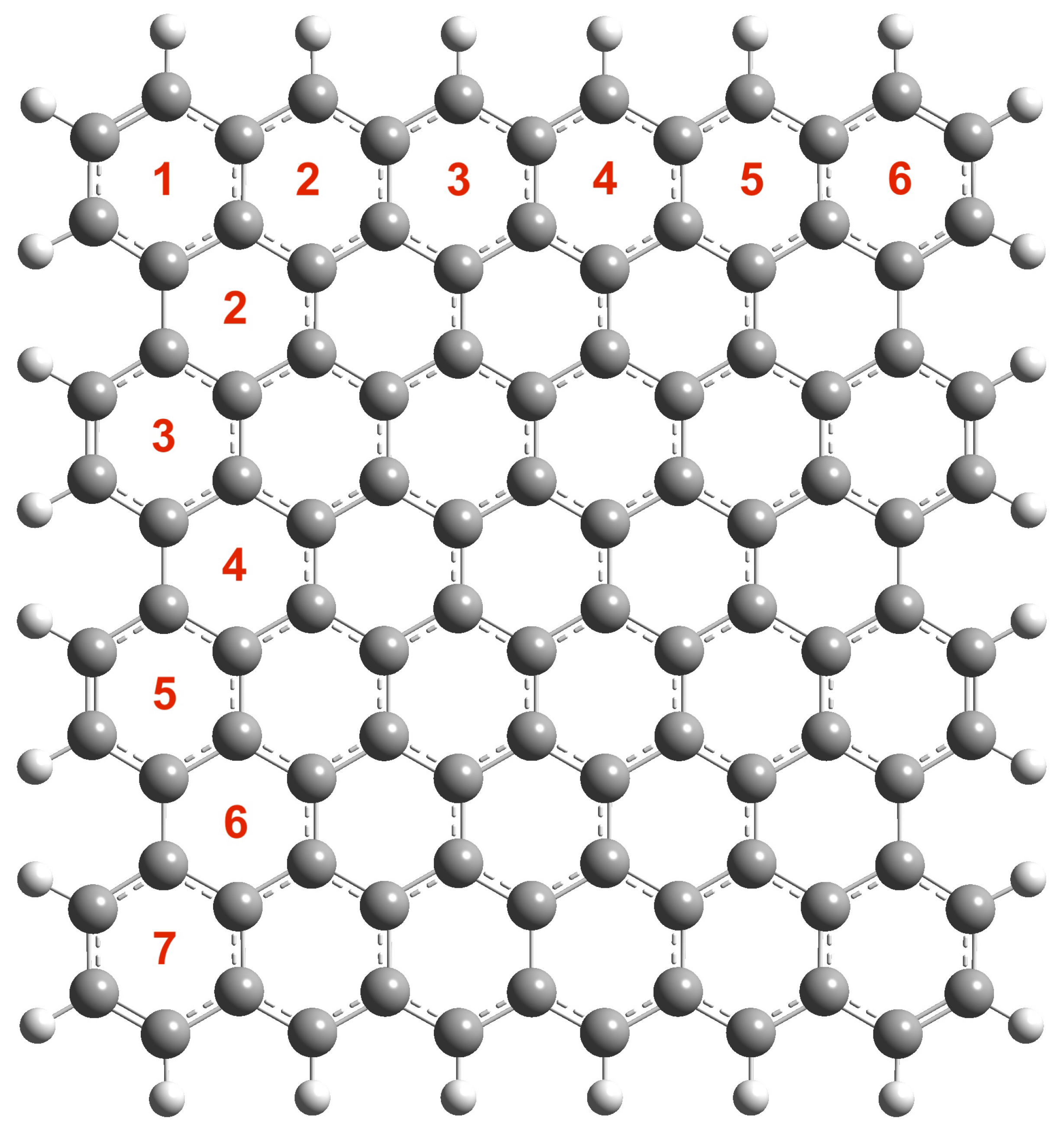
2.1. Theoretical Model
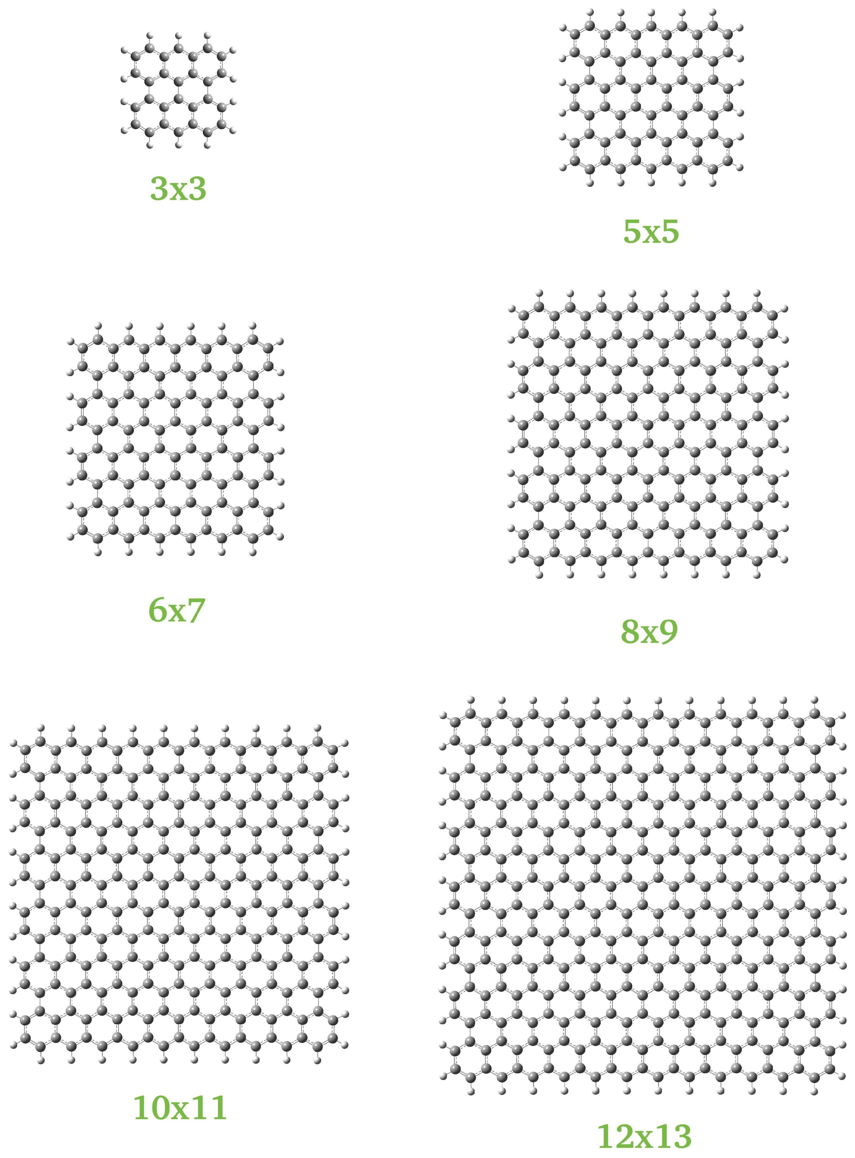
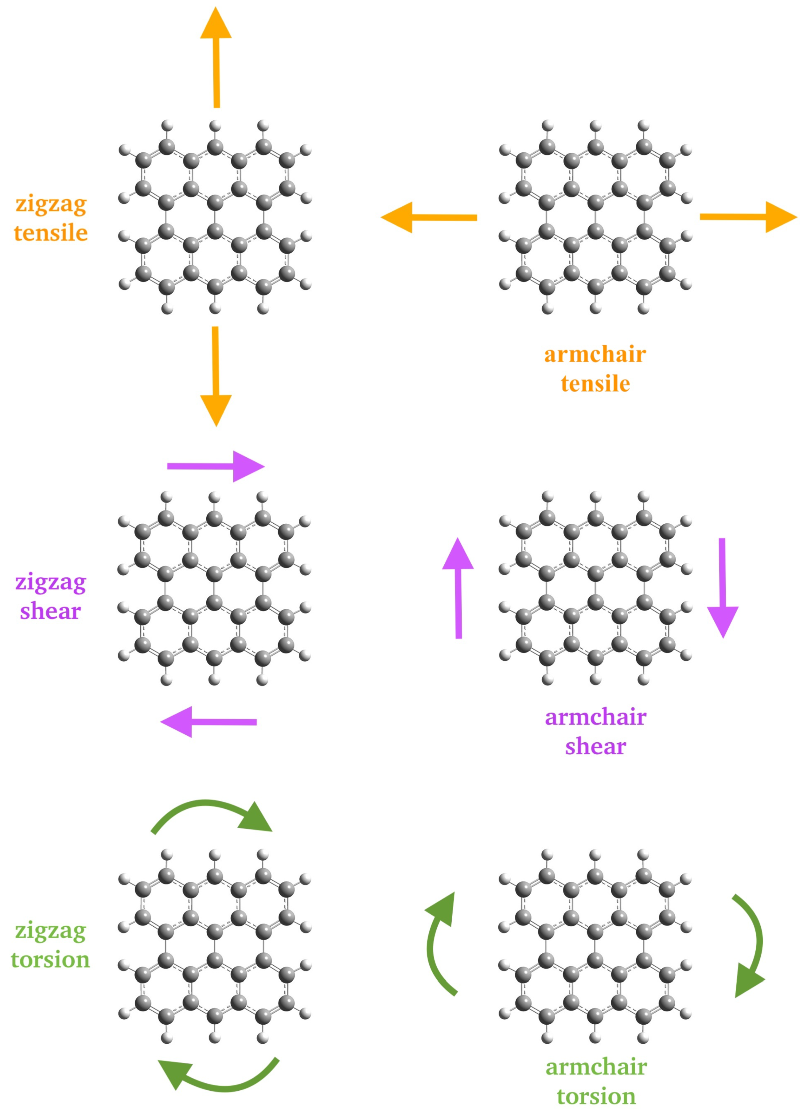
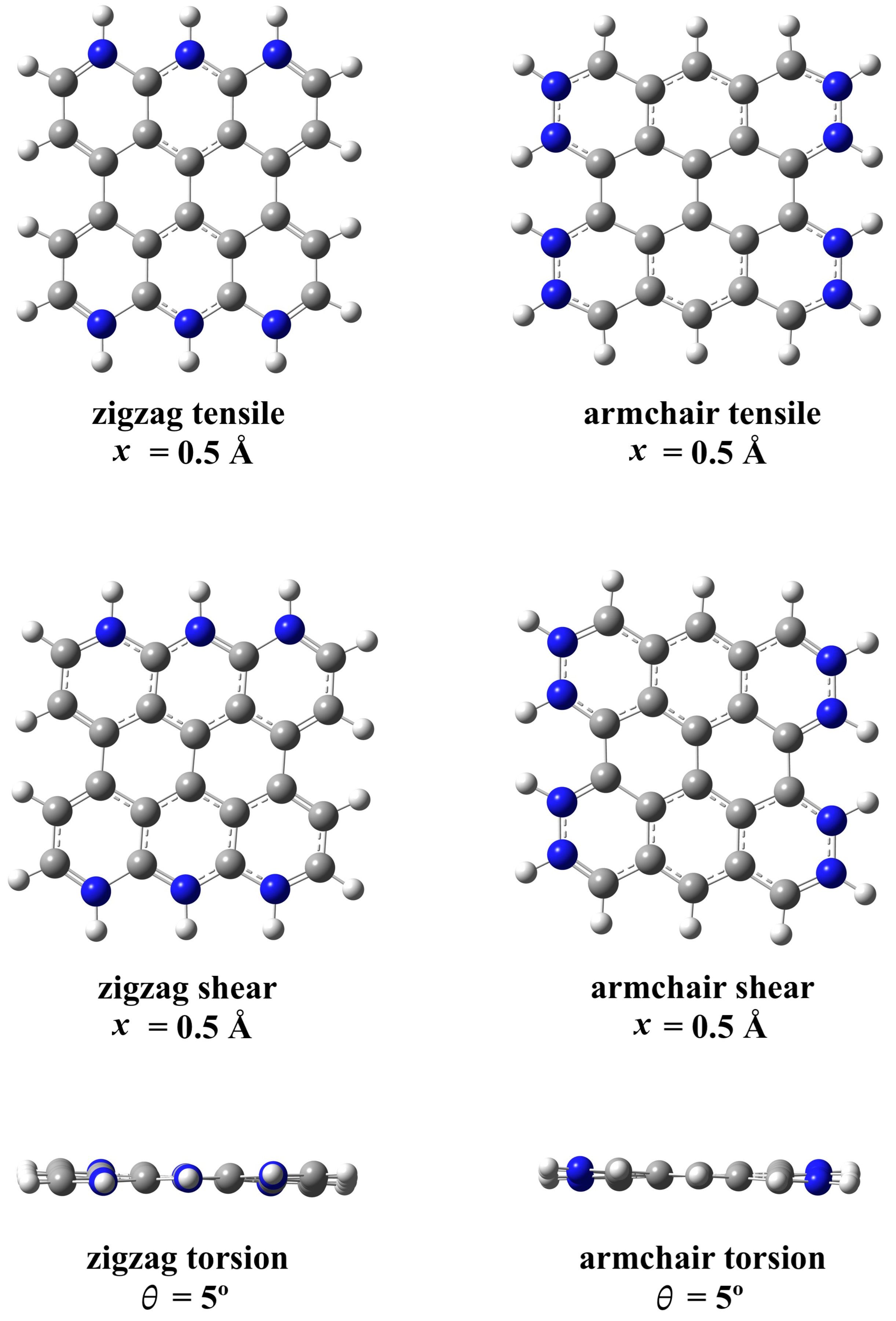
2.2. Systems Studied
2.3. Computational Method
3. Results
3.1. Young’s Modulus
3.2. Shear Modulus
3.3. Torsion Constant
3.4. Poisson’s Ratio
4. Conclusions
Author Contributions
Funding
Institutional Review Board Statement
Informed Consent Statement
Data Availability Statement
Conflicts of Interest
References
- Bissett, M.A.; Tsuji, M.; Ago, H. Strain engineering the properties of graphene and other two-dimensional crystals. Phys. Chem. Chem. Phys. 2014, 16, 11124–11138. [Google Scholar] [CrossRef]
- Deng, S.; Sumant, A.V.; Berry, V. Strain engineering in two-dimensional nanomaterials beyond graphene. Nano Today 2018, 22, 14–35. [Google Scholar] [CrossRef]
- Peng, Z.; Chen, X.; Fan, Y.; Srolovitz, D.J.; Lei, D. Strain engineering of 2D semiconductors and graphene: From strain fields to band-structure tuning and photonic applications. Light. Sci. Appl. 2020, 9, 190. [Google Scholar] [CrossRef] [PubMed]
- Ge, X.; Zhou, X.; Sun, D.; Chen, X. First-Principles Study of Structural and Electronic Properties of Monolayer PtX2 and Janus PtXY (X, Y = S, Se, and Te) via Strain Engineering. ACS Omega 2023, 8, 5715–5721. [Google Scholar] [CrossRef]
- Qi, Y.; Sadi, M.A.; Hu, D.; Zheng, M.; Wu, Z.; Jiang, Y.; Chen, Y.P. Recent Progress in Strain Engineering on Van der Waals 2D Materials: Tunable Electrical, Electrochemical, Magnetic, and Optical Properties. Adv. Mater. 2023, 35, 2205714. [Google Scholar] [CrossRef]
- Hasani, N.; Rajabi-Maram, A.; Touski, S.B. Strain engineering of electronic and spin properties in SnX (X = P, As, Sb, Bi) monolayers. J. Phys. Chem. Solids 2023, 174, 111131. [Google Scholar] [CrossRef]
- Kim, J.M.; Haque, M.F.; Hsieh, E.Y.; Nahid, S.M.; Zarin, I.; Jeong, K.Y.; So, J.P.; Park, H.G.; Nam, S. Strain Engineering of Low-Dimensional Materials for Emerging Quantum Phenomena and Functionalities. Adv. Mater. 2023, 35, 2107362. [Google Scholar] [CrossRef] [PubMed]
- Pandey, M.; Pandey, C.; Ahuja, R.; Kumar, R. Straining techniques for strain engineering of 2D materials towards flexible straintronic applications. Nano Energy 2023, 109, 108278. [Google Scholar] [CrossRef]
- Fan, W.; Winands, T.; Doltsinis, N.L.; Li, Y.; Wang, Z. A Decatwistacene with an Overall 170° Torsion. Angew. Chem. Int. Ed. 2017, 56, 15373–15377. [Google Scholar] [CrossRef]
- Liu, H.; Lee, M.; Šiškins, M.; van der Zant, H.S.J.; Steeneken, P.G.; Verbiest, G.J. Tuning heat transport in graphene by tension. Phys. Rev. B 2023, 108, L081401. [Google Scholar] [CrossRef]
- He, S.; Zhang, Y.; Gao, J.; Nag, A.; Rahaman, A. Integration of Different Graphene Nanostructures with PDMS to Form Wearable Sensors. Nanomaterials 2022, 12, 950. [Google Scholar] [CrossRef]
- Srimaneepong, V.; Skallevold, H.E.; Khurshid, Z.; Zafar, M.S.; Rokaya, D.; Sapkota, J. Graphene for Antimicrobial and Coating Application. Int. J. Mol. Sci. 2022, 23, 499. [Google Scholar] [CrossRef]
- Zhang, Y.; Jin, Y.; Liu, J.; Ren, Q.; Chen, Z.; Zhao, Y.; Zhao, P. Strain engineering of graphene on rigid substrates. Nanoscale Adv. 2022, 4, 5056–5061. [Google Scholar] [CrossRef] [PubMed]
- de-la Huerta-Sainz, S.; Ballesteros, A.; Cordero, N.A. Quantum Revivals in Curved Graphene Nanoflakes. Nanomaterials 2022, 12, 1953. [Google Scholar] [CrossRef]
- Yuan, X.; Zhu, S. Compressive strain engineering of strong and sensitive pseudomagnetic fields in buckled graphene nanobubbles. Phys. Rev. B 2023, 107, 195417. [Google Scholar] [CrossRef]
- De Beule, C.; Phong, V.T.; Mele, E.J. Network model for periodically strained graphene. Phys. Rev. B 2023, 107, 045405. [Google Scholar] [CrossRef]
- Mahmud, M.T.; Zhai, D.; Sandler, N. Topological Flat Bands in Strained Graphene: Substrate Engineering and Optical Control. Nano Lett. 2023, 23, 7725–7732. [Google Scholar] [CrossRef]
- Dawood, O.M.; Thameel, M.N.; Mohammad, J. Unveiling a new Raman active mode in graphene and its implications for band gap formation: A DFT study. Phys. E Low-Dimens. Syst. Nanostruct. 2023, 154, 115810. [Google Scholar] [CrossRef]
- Tepliakov, N.V.; Lischner, J.; Kaxiras, E.; Mostofi, A.A.; Pizzochero, M. Unveiling and Manipulating Hidden Symmetries in Graphene Nanoribbons. Phys. Rev. Lett. 2023, 130, 026401. [Google Scholar] [CrossRef]
- Park, H.C.; Han, J.; Myoung, N. A strain-engineered graphene qubit in a nanobubble. Quantum Sci. Technol. 2023, 8, 025012. [Google Scholar] [CrossRef]
- Lee, H.C.; Hsieh, E.Y.; Yong, K.; Nam, S. Multiaxially-stretchable kirigami-patterned mesh design for graphene sensor devices. Nano Res. 2020, 13, 1406–1412. [Google Scholar] [CrossRef]
- Chun, S.; Choi, Y.; Park, W. All-graphene strain sensor on soft substrate. Carbon 2017, 116, 753–759. [Google Scholar] [CrossRef]
- Cong, L.; Yuan, Z.; Bai, Z.; Wang, X.; Zhao, W.; Gao, X.; Hu, X.; Liu, P.; Guo, W.; Li, Q.; et al. On-chip torsion balances with femtonewton force resolution at room temperature enabled by carbon nanotube and graphene. Sci. Adv. 2021, 7, eabd2358. [Google Scholar] [CrossRef]
- Foroughi, J.; Spinks, G. Carbon nanotube and graphene fiber artificial muscles. Nanoscale Adv. 2019, 1, 4592–4614. [Google Scholar] [CrossRef] [PubMed]
- Malisz, K.; Świeczko Żurek, B. Graphene Production and Biomedical Applications: A Review. Crystals 2023, 13, 1413. [Google Scholar] [CrossRef]
- Cordero, N.A.; Alonso, J.A. Interaction of Surfactants Containing a Sulfuric Group with a (5,5) Carbon Nanotube. J. Phys. Chem. 2010, 114, 17249–17256. [Google Scholar] [CrossRef]
- García, T.; Rodríguez-Bolívar, S.; Cordero, N.A.; Romera, E. Wavepacket revivals in monolayer and bilayer graphene rings. J. Phys. Condens. Matter 2013, 25, 235301. [Google Scholar] [CrossRef]
- García, T.; Cordero, N.A.; Romera, E. Zitterbewegung and quantum revivals in monolayer graphene quantum dots in magnetic fields. Phys. Rev. B 2014, 89, 075416. [Google Scholar] [CrossRef]
- Yakobson, B.I.; Brabec, C.J.; Bernholc, J. Nanomechanics of Carbon Tubes: Instabilities beyond Linear Response. Phys. Rev. Lett. 1996, 76, 2511–2514. [Google Scholar] [CrossRef]
- Reddy, C.D.; Rajendran, S.; Liew, K.M. Equilibrium configuration and continuum elastic properties of finite sized graphene. Nanotechnology 2006, 17, 864. [Google Scholar] [CrossRef]
- Ru, C.Q. Effect of van der Waals forces on axial buckling of a double-walled carbon nanotube. J. Appl. Phys. 2000, 87, 7227–7231. [Google Scholar] [CrossRef]
- El Kass, D.; Monneau, R. Atomic to continuum passage for nanotubes: A discrete Saint-Venant principle and error estimates. Arch. Ration. Mech. Anal. 2014, 213, 25–128. [Google Scholar] [CrossRef]
- Huang, K.; Yin, Y.; Qu, B. Tight-binding theory of graphene mechanical properties. Microsyst. Technol. 2021, 27, 3851–3858. [Google Scholar] [CrossRef]
- Anastasi, A.A.; Ritos, K.; Cassar, G.; Borg, M.K. Mechanical properties of pristine and nanoporous graphene. Mol. Simul. 2016, 42, 1502–1511. [Google Scholar] [CrossRef]
- Cho, J.; Luo, J.; Daniel, I. Mechanical characterization of graphite/epoxy nanocomposites by multi-scale analysis. Compos. Sci. Technol. 2007, 67, 2399–2407. [Google Scholar] [CrossRef]
- Min, K.; Aluru, N.R. Mechanical properties of graphene under shear deformation. Appl. Phys. Lett. 2011, 98, 013113. [Google Scholar] [CrossRef]
- Sakhaee-Pour, A. Elastic properties of single-layered graphene sheet. Solid State Commun. 2009, 149, 91–95. [Google Scholar] [CrossRef]
- Tsai, J.L.; Tu, J.F. Characterizing mechanical properties of graphite using molecular dynamics simulation. Mater. Des. 2010, 31, 194–199. [Google Scholar] [CrossRef]
- Zakharchenko, K.V.; Katsnelson, M.I.; Fasolino, A. Finite Temperature Lattice Properties of Graphene beyond the Quasiharmonic Approximation. Phys. Rev. Lett. 2009, 102, 046808. [Google Scholar] [CrossRef]
- Chandra, Y.; Adhikari, S.; Mukherjee, S.; Mukhopadhyay, T. Unfolding the mechanical properties of buckypaper composites: Nano- to macro-scale coupled atomistic-continuum simulations. Eng. Comput. 2022, 38, 5199–5229. [Google Scholar] [CrossRef]
- Savin, A.; Korznikova, E.; Dmitriev, S. Improving bending rigidity of graphene nanoribbons by twisting. Mech. Mater. 2019, 137, 103123. [Google Scholar] [CrossRef]
- Thakur, R.; Ahluwalia, P.; Kumar, A.; Sharma, M.; Sharma, R. Twisted helical armchair graphene nanoribbons: Mechanical and electronic properties. Eur. Phys. J. 2021, 94, 99. [Google Scholar] [CrossRef]
- Sun, Y.W.; Papageorgiou, D.G.; Humphreys, C.J.; Dunstan, D.J.; Puech, P.; Proctor, J.E.; Bousige, C.; Machon, D.; San-Miguel, A. Mechanical properties of graphene. Appl. Phys. Rev. 2021, 8, 021310. [Google Scholar] [CrossRef]
- Ragab, T.; McDonald, J.; Basaran, C. Aspect ratio effect on shear modulus and ultimate shear strength of graphene nanoribbons. Diam. Relat. Mater. 2017, 74, 9–15. [Google Scholar] [CrossRef]
- Landau, L.; Lifshitz, E. Theory of Elasticity; Pergamon Press: Oxford, UK, 1970. [Google Scholar]
- Timoshenko, S.; Goodier, J. Theory of Elasticity; McGRAW-HILL: New York, NY, USA, 1951. [Google Scholar]
- Shodja, H.M.; Ojaghnezhad, F.; Etehadieh, A.; Tabatabaei, M. Elastic moduli tensors, ideal strength, and morphology of stanene based on an enhanced continuum model and first principles. Mech. Mater. 2017, 110, 1–15. [Google Scholar] [CrossRef]
- Guo, C.; Papangelis, J. Torsion of beams with corrugated webs. In Proceedings of the Ninth International Conference on Advances in Steel Structures (ICASS 2018), Hong Kong, China, 5–7 December 2018; pp. 5–7. [Google Scholar] [CrossRef]
- Trahair, N.; Bradford, M.; Nethercot, D.; Gardner, L. The Behaviour and Design of Steel Structures to EC3, 4th ed.; Taylor & Francis: New York, NY, USA, 2008. [Google Scholar]
- Xia, D.; Li, Q.; Xue, Q.; Liang, C.; Dong, M. Super flexibility and stability of graphene nanoribbons under severe twist. Phys. Chem. Chem. Phys. 2016, 18, 18406–18413. [Google Scholar] [CrossRef]
- Shi, J.X.; Natsuki, T.; Lei, X.W.; Ni, Q.Q. Equivalent Young’s modulus and thickness of graphene sheets for the continuum mechanical models. Appl. Phys. Lett. 2014, 104, 223101. [Google Scholar] [CrossRef]
- Lee, D.H.; Lee, M.J.; Kim, Y.S.; Choi, J.S.; Park, B.H. Sample rotation angle dependence of graphene thickness measured using atomic force microscope. Carbon 2015, 81, 210–215. [Google Scholar] [CrossRef]
- Delfani, M.R.; Shodja, H. Dual ideal shear strengths for chiral single-walled carbon nanotubes. Int. J.-Non-Linear Mech. 2020, 120, 103382. [Google Scholar] [CrossRef]
- Huang, Y.; Wu, J.; Hwang, K.C. Thickness of graphene and single-wall carbon nanotubes. Phys. Rev. B 2006, 74, 245413. [Google Scholar] [CrossRef]
- Stewart, J. Optimization of parameters for semiempirical methods VI: More modifications to the NDDO approximations and re-optimization of parameters. J. Mol. Model. 2013, 19, 1–32. [Google Scholar] [CrossRef] [PubMed]
- Frisch, M.J.; Trucks, G.W.; Schlegel, H.B.; Scuseria, G.E.; Robb, M.A.; Cheeseman, J.R.; Scalmani, G.; Barone, V.; Petersson, G.A.; Nakatsuji, H.; et al. Gaussian 16; Revision C.01; Gaussian Inc.: Wallingford, CT, USA, 2019. [Google Scholar]
- Throssel, K. Evaluating and Improving Approximate LCAO-MO Theory with Restored Overlap and Bond Order Bond Energy Corrections. Ph.D. Thesis, Wesleyan University, Middletown, CT, USA, 2017. Available online: https://digitalcollections.wesleyan.edu/object/ir-2308 (accessed on 24 March 2024).
- Jurkiewicz, K.; Hawelek, L.; Balin, K.; Szade, J.; Braghiroli, F.L.; Fierro, V.; Celzard, A.; Burian, A. Conversion of Natural Tannin to Hydrothermal and Graphene-Like Carbons Studied by Wide-Angle X-ray Scattering. J. Phys. Chem. A 2015, 119, 8692–8701. [Google Scholar] [CrossRef] [PubMed]
- Jaiyong, P.; Bryce, R.A. Approximate quantum chemical methods for modelling carbohydrate conformation and aromatic interactions: β-cyclodextrin and its adsorption on a single-layer graphene sheet. Phys. Chem. Chem. Phys. 2017, 19, 15346–15355. [Google Scholar] [CrossRef] [PubMed]
- Vorontsov, A.V.; Tretyakov, E.V. Determination of graphene’s edge energy using hexagonal graphene quantum dots and PM7 method. Phys. Chem. Chem. Phys. 2018, 20, 14740–14752. [Google Scholar] [CrossRef] [PubMed]
- Hariharan, S.; Majumder, M.; Edel, R.; Grabnic, T.; Sibener, S.J.; Hase, W.L. Exploratory Direct Dynamics Simulations of 3O2 Reaction with Graphene at High Temperatures. J. Phys. Chem. C 2018, 122, 29368–29379. [Google Scholar] [CrossRef]
- Bertorelle, F.; Basu, S.; Fakhouri, H.; Bakulic, M.P.; Mignon, P.; Russier-Antoine, I.; Brevet, P.F.; Thomas, S.; Kalarikkal, N.; Antoine, R. Covalent anchoring of atomically precise glutathione-protected gold nanoclusters on graphene oxide nanosheets. Nano Express 2020, 1, 030005. [Google Scholar] [CrossRef]
- Gun’ko, V. Quantum-chemically computed integral characteristics of complex nanomaterials. Chem. Phys. Technol. Surf./Khimiya Fiz. Tekhnologiya Poverhni 2021, 12, 157–167. Available online: https://www.cpts.com.ua/index.php/cpts/article/download/590/598 (accessed on 24 March 2024). [CrossRef]
- Chi, S.C.; Lee, C.L.; Chang, C.M. Adsorption of Pesticides, Antibiotics and Microcystin-LR by Graphene and Hexagonal Boron Nitride Nano-Systems: A Semiempirical PM7 and Theoretical HSAB Study. Crystals 2022, 12, 1068. [Google Scholar] [CrossRef]
- Tromer, R.M.; Felix, I.M.; Pereira, L.F.C.; da Luz, M.G.E.; Junior, L.A.R.; Galvão, D.S. Lattice thermal conductivity of 2D nanomaterials: A simple semi-empirical approach. Phys. Chem. Chem. Phys. 2023, 25, 28703–28715. [Google Scholar] [CrossRef]
- Lebedeva, I.V.; Minkin, A.S.; Popov, A.M.; Knizhnik, A.A. Elastic constants of graphene: Comparison of empirical potentials and DFT calculations. Phys. E Low-Dimens. Syst. Nanostruct. 2019, 108, 326–338. [Google Scholar] [CrossRef]
- Giannopoulos, G.I. Elastic buckling and flexural rigidity of graphene nanoribbons by using a unique translational spring element per interatomic interaction. Comput. Mater. Sci. 2012, 53, 388–395. [Google Scholar] [CrossRef]
- Scarpa, F.; Adhikari, S.; Phani, A.S. Effective elastic mechanical properties of single layer graphene sheets. Nanotechnology 2009, 20, 065709. [Google Scholar] [CrossRef] [PubMed]
- Polyakova, P.; Galiakhmetova, L.K.; Murzaev, R.; Lisovenko, D.; Baimova, J. Elastic properties of diamane. Lett. Mater. 2023, 13, 171–176. [Google Scholar] [CrossRef]
- Tzeng, S.H.; Tsai, J.L. Characterizing the Mechanical Properties of Graphene and Single Walled Carbon Nanotubes. J. Mech. 2011, 27, 461–467. [Google Scholar] [CrossRef]
- Zhang, Y.; Huang, L.; Huang, J. A modified spring finite element model for graphene elastic properties study. Mater. Today Commun. 2023, 34, 105158. [Google Scholar] [CrossRef]
- Sha’bani, F.; Rash-Ahmadi, S. Length scale effect on the buckling behavior of a graphene sheets using modified couple stress theory and molecular dynamics method. Acta Mech. 2022, 233, 943–960. [Google Scholar] [CrossRef]
- Zaeri, M.; Ziaei-Rad, S.; Vahedi, A.; Karimzadeh, F. Mechanical modelling of carbon nanomaterials from nanotubes to buckypaper. Carbon 2010, 48, 3916–3930. [Google Scholar] [CrossRef]
- Tapia, A.; Peón-Escalante, R.; Villanueva, C.; Avilés, F. Influence of vacancies on the elastic properties of a graphene sheet. Comput. Mater. Sci. 2012, 55, 255–262. [Google Scholar] [CrossRef]
- Tahani, M.; Safarian, S. Determination of rigidities, stiffness coefficients and elastic constants of multi-layer graphene sheets by an asymptotic homogenization method. J. Braz. Soc. Mech. Sci. Eng. 2019, 41, 1–16. [Google Scholar] [CrossRef]
- Lee, C.; Wei, X.; Kysar, J.W.; Hone, J. Measurement of the Elastic Properties and Intrinsic Strength of Monolayer Graphene. Science 2008, 321, 385–388. [Google Scholar] [CrossRef]
- Blakslee, O.L.; Proctor, D.G.; Seldin, E.J.; Spence, G.B.; Weng, T. Elastic Constants of Compression-Annealed Pyrolytic Graphite. J. Appl. Phys. 2003, 41, 3373–3382. [Google Scholar] [CrossRef]
- Lengvarskỳ, P.; Bocko, J. Mechanical Properties and Eigenfrequencies of Graphene Sheets. Acta Mech. Slovaca 2017, 21, 26–32. [Google Scholar] [CrossRef]
- Thomas, S.; Ajith, K.; Lee, S.U.; Valsakumar, M.C. Assessment of the mechanical properties of monolayer graphene using the energy and strain-fluctuation methods. RSC Adv. 2018, 8, 27283–27292. [Google Scholar] [CrossRef] [PubMed]
- Liu, X.; Metcalf, T.H.; Robinson, J.T.; Houston, B.H.; Scarpa, F. Shear Modulus of Monolayer Graphene Prepared by Chemical Vapor Deposition. Nano Lett. 2012, 12, 1013–1017. [Google Scholar] [CrossRef]
- Mukhopadhyay, T.; Mahata, A.; Adhikari, S.; Asle Zaeem, M. Probing the shear modulus of two-dimensional multiplanar nanostructures and heterostructures. Nanoscale 2018, 10, 5280–5294. [Google Scholar] [CrossRef]
- Georgantzinos, S.; Giannopoulos, G.; Anifantis, N. Numerical investigation of elastic mechanical properties of graphene structures. Mater. Des. 2010, 31, 4646–4654. [Google Scholar] [CrossRef]
- Zheng, W.; Guo, Z.; Wang, Z.; Boay, C.G.; Wang, X.; Li, Y. Modeling analysis of elastic properties of graphene-carbon nanotube (G-C) reinforced composites. Polym. Compos. 2022, 43, 3136–3149. [Google Scholar] [CrossRef]
- Lindahl, N.; Midtvedt, D.; Svensson, J.; Nerushev, O.A.; Lindvall, N.; Isacsson, A.; Campbell, E.E.B. Determination of the Bending Rigidity of Graphene via Electrostatic Actuation of Buckled Membranes. Nano Lett. 2012, 12, 3526–3531. [Google Scholar] [CrossRef]
- Androulidakis, C.; Zhang, K.; Robertson, M.; Tawfick, S. Tailoring the mechanical properties of 2D materials and heterostructures. 2D Mater. 2018, 5, 032005. [Google Scholar] [CrossRef]
- Androulidakis, C.; Koukaras, E.; Hadjinicolaou, M.; Galiotis, C. Non-Eulerian behavior of graphitic materials under compression. Carbon 2018, 138, 227–233. [Google Scholar] [CrossRef]
- Androulidakis, C.; Koukaras, E.N.; Sampathkumar, K.; Rahova, J.; Galiotis, C.; Frank, O. Hierarchy of nanoscale graphene wrinkles on compliant substrate: Theory and experiment. Extrem. Mech. Lett. 2020, 40, 100948. [Google Scholar] [CrossRef]
- Duan, W.H.; Wang, C.M. Nonlinear bending and stretching of a circular graphene sheet under a central point load. Nanotechnology 2009, 20, 075702. [Google Scholar] [CrossRef] [PubMed]
- Kudin, K.N.; Scuseria, G.E.; Yakobson, B.I. C2F, BN, and C nanoshell elasticity from ab initio computations. Phys. Rev. B 2001, 64, 235406. [Google Scholar] [CrossRef]
- Wang, L.; Zheng, Q.; Liu, J.Z.; Jiang, Q. Size Dependence of the Thin-Shell Model for Carbon Nanotubes. Phys. Rev. Lett. 2005, 95, 105501. [Google Scholar] [CrossRef] [PubMed]
- Shenderova, O.A.; Zhirnov, V.V.; Brenner, D.W. Carbon Nanostructures. Crit. Rev. Solid State Mater. Sci. 2002, 27, 227–356. [Google Scholar] [CrossRef]
- Pine, P.; Yaish, Y.E.; Adler, J. Vibrational analysis of thermal oscillations of single-walled carbon nanotubes under axial strain. Phys. Rev. B 2014, 89, 115405. [Google Scholar] [CrossRef]
- Shen, H. Mechanical properties and thermal conductivity of the twisted graphene nanoribbons. Mol. Phys. 2014, 112, 2614–2620. [Google Scholar] [CrossRef]
- Chatzidakis, G.D.; Kalosakas, G.; Fthenakis, Z.G.; Lathiotakis, N.N. A torsional potential for graphene derived from fitting to DFT results. Eur. Phys. J. B 2018, 91, 11. [Google Scholar] [CrossRef]
- Yoneyama, K.; Yamanaka, A.; Okada, S. Energetics and electronic structure of graphene nanoribbons under uniaxial torsional strain. Jpn. J. Appl. Phys. 2019, 58, SDDD05. [Google Scholar] [CrossRef]
- Tapia, A.; Cab, C.; Hernández-Pérez, A.; Villanueva, C.; Peñuñuri, F.; Avilés, F. The bond force constants and elastic properties of boron nitride nanosheets and nanoribbons using a hierarchical modeling approach. Phys. E Low-Dimens. Syst. Nanostruct. 2017, 89, 183–193. [Google Scholar] [CrossRef]
- Sakharova, N.A.; Pereira, A.F.G.; Antunes, J.M. A Study of the Mechanical Behaviour of Boron Nitride Nanosheets Using Numerical Simulation. Nanomaterials 2023, 13, 2759. [Google Scholar] [CrossRef]
- Jiang, J.W.; Chang, T.; Guo, X.; Park, H.S. Intrinsic negative Poisson’s ratio for single-layer graphene. Nano Lett. 2016, 16, 5286–5290. [Google Scholar] [CrossRef] [PubMed]
- Wang, Y.; Lei, J.; Liu, Z. Molecular dynamics study on the anisotropic Poisson’s ratio of the graphene. Diam. Relat. Mater. 2019, 93, 66–74. [Google Scholar] [CrossRef]
- Caillerie, D.; Mourad, A.; Raoult, A. Discrete homogenization in graphene sheet modeling. J. Elast. 2006, 84, 33–68. [Google Scholar] [CrossRef]
- Cadelano, E.; Palla, P.L.; Giordano, S.; Colombo, L. Nonlinear Elasticity of Monolayer Graphene. Phys. Rev. Lett. 2009, 102, 235502. [Google Scholar] [CrossRef] [PubMed]
- Lu, Q.; Huang, R. Nonlinear mechanics of single-atomic-layer graphene sheets. Int. J. Appl. Mech. 2009, 1, 443–467. [Google Scholar] [CrossRef]
- Koberidze, M. Computational Studies of Torsional Properties of Single-Walled Carbon Nanotubes. Master’s Thesis, University of Jyväskylä, Jyväskylä, Findland, 2010. Available online: https://jyx.jyu.fi/handle/123456789/37243 (accessed on 24 March 2024).
- Politano, A.; Marino, A.R.; Campi, D.; Farías, D.; Miranda, R.; Chiarello, G. Elastic properties of a macroscopic graphene sample from phonon dispersion measurements. Carbon 2012, 50, 4903–4910. [Google Scholar] [CrossRef]

| Nanoflake | Aspect Ratio | Edge | Edge Length/Å | E/TPa |
|---|---|---|---|---|
| 3 × 3 | 1.03 | zigzag | 7.099 | 0.927 |
| armchair | 7.288 | 1.224 | ||
| 5 × 5 | 1.07 | zigzag | 11.368 | 0.869 |
| armchair | 12.191 | 1.229 | ||
| 6 × 7 | 0.94 | zigzag | 15.618 | 1.061 |
| armchair | 14.667 | 1.200 | ||
| 8 × 9 | 0.98 | zigzag | 19.879 | 1.105 |
| armchair | 19.580 | 1.220 | ||
| 10 × 11 | 1.01 | zigzag | 24.143 | 1.217 |
| armchair | 24.484 | 1.134 | ||
| 12 × 13 | 1.04 | zigzag | 28.388 | 1.127 |
| armchair | 29.409 | 1.205 |
| Source | E/TPa | Method | h/Å |
|---|---|---|---|
| Reddy et al. [30] | 0.671 | interatomic potential | 3.4 |
| Lebedeva et al. [66] | 0.7058–1.343 (depending on the potential used) | interatomic potential | 3.34 |
| Giannopoulos [67] | 0.745208 for zigzag graphene nanoribons | spring-based structural mechanics | N/A |
| Giannopoulos [67] | 0.745204 for armchair graphene nanoribbons | spring-based structural mechanics | N/A |
| Scarpa et al. [68] | 0.762–1.000 (depending on the potential used) | cellular material mechanics theory | 0.74–0.84 |
| Polyakova et al. [69] | 0.820 | molecular dynamics | N/A |
| Tsai and Tu [38] | 0.912 | molecular dynamics | 3.4 |
| Tzeng and Tsai [70] | 0.912 | molecular dynamics | 3.4 |
| Zhang et al. [71] | 0.985 | spring finite element model | N/A |
| Sakhaee-Pour [37] | 1.040 for zigzag graphene | interatomic potential | 3.4 |
| Sakhaee-Pour [37] | 1.042 for armchair graphene | interatomic potential | 3.4 |
| Sha’bani and Rash-Ahmadi [72] | 1.05 | molecular dynamics | N/A |
| Zaeri et al. [73] | 1.040 | molecular structural mechanics finite element method | 3.4 |
| Tapia et al. [74] | 1.042 | atomistic finite element method | 3.4 |
| Anastasi et al. [34] | 1.061 for zigzag graphene | molecular dynamics | 3.35 |
| Anastasi et al. [34] | 1.035 for armchair graphene | molecular dynamics | 3.35 |
| Chandra et al. [40] | 1.082 | atomistic finite element method | 1.46 |
| Tahani and Safarian [75] | 1.13 | homogenization composite shell model | N/A |
| Cho et al. [35] | 1.153 for graphite | molecular mechanics | 3.35 |
| Shi et al. [51] | 2.81 | atomic interaction based continuum model | 1.27 |
| Nanoflake | Average C–C Distance | Percentage of Edge C Atoms | |
|---|---|---|---|
| Central Ring | Edge | ||
| 5 × 5 | 1.420 | 1.399 | 58 % |
| 6 × 7 | 1.418 | 1.402 | 48 % |
| 10 × 11 | 1.418 | 1.403 | 33 % |
| Nanoflake | Edge | G/GPa |
|---|---|---|
| 3 × 3 | zigzag | 221 |
| armchair | 255 | |
| 5 × 5 | zigzag | 226 |
| armchair | 259 | |
| 6 × 7 | zigzag | 189 |
| armchair | 288 | |
| 8 × 9 | zigzag | 263 |
| armchair | 279 | |
| 10 × 11 | zigzag | 222 |
| armchair | 240 | |
| 12 × 13 | zigzag | 229 |
| armchair | 250 |
| Source | G/GPa | Method | h/Å |
|---|---|---|---|
| Mukhopadhyay et al. [81] | 125.4 | molecular mechanics | 3.4 |
| Scarpa et al. [68] | 202–270 (depending on the potential used) | cellular material mechanics theory | 0.74–0.84 |
| Tahani and Safarian [75] | 212 | homogenization composite shell model | N/A |
| Sakhaee-Pour [37] | 213 for zigzag graphene | interatomic potential | 3.4 |
| Sakhaee-Pour [37] | 228 for armchair graphene | interatomic potential | 3.4 |
| Tapia et al. [74] | 213 | atomistic finite element method | 3.4 |
| Zhang et al. [71] | 242 | spring-based finite element model | N/A |
| Georgantzinos et al. [82] | 280 | spring-based finite element model | 3.4 |
| Polyakova et al. [69] | 302 | molecular dynamics | N/A |
| Reddy et al. [30] | 384 | interatomic potential | 3.4 |
| Tsai and Tu [38] | 358 | molecular dynamics | 3.4 |
| Zheng et al. [83] | 434 | beam finite element method | 3.4 |
| Zakharchenko et al. [39] | 445 | atomistic Monte Carlo based on empirical bond order potential | N/A |
| Min and Aluru [36] | ≈460 for zigzag graphene | molecular dynamics | 3.335 |
| Min and Aluru [36] | ≈360 for armchair graphene | molecular dynamics | 3.335 |
| Cho et al. [35] | 482 for graphite | molecular mechanics | 3.35 |
| Zaeri et al. [73] | 490 | molecular structural mechanics finite element method | 3.4 |
| Chandra et al. [40] | 606 | atomistic finite element method | 1.46 |
| Nanoflake | Edge | J/( ) | /Å | |
|---|---|---|---|---|
| Equation (11) | Equation (12) | |||
| 3 × 3 | zigzag | 3.89 | 64.9 | 0.71 |
| armchair | 7.02 | 62.6 | 0.98 | |
| 5 × 5 | zigzag | 10.0 | 126 | 0.88 |
| armchair | 6.76 | 116 | 0.75 | |
| 6 × 7 | zigzag | 10.1 | 157 | 0.80 |
| armchair | 12.2 | 169 | 0.85 | |
| 8 × 9 | zigzag | 7.08 | 219 | 0.58 |
| armchair | 12.6 | 223 | 0.76 | |
| 10 × 11 | zigzag | 16.6 | 280 | 0.79 |
| armchair | 22.2 | 276 | 0.92 | |
| 12 × 13 | zigzag | 28.7 | 342 | 0.94 |
| armchair | 30.1 | 329 | 0.99 | |
| Nanoflake | Edge | ||
|---|---|---|---|
| Equation (13) | Equation (14) | ||
| 3 × 3 | zigzag | 0.33 | 1.09 |
| armchair | 0.43 | 1.40 | |
| 5 × 5 | zigzag | 0.30 | 0.93 |
| armchair | 0.39 | 1.38 | |
| 6 × 7 | zigzag | 0.33 | 1.81 |
| armchair | 0.35 | 1.09 | |
| 8 × 9 | zigzag | 0.31 | 1.10 |
| armchair | 0.34 | 1.19 | |
| 10 × 11 | zigzag | 0.31 | 1.74 |
| armchair | 0.36 | 1.36 | |
| 12 × 13 | zigzag | 0.31 | 1.46 |
| armchair | 0.33 | 1.41 | |
| Source | Method | |
|---|---|---|
| Tapia et al. [74] | 0.072 | atomistic finite element method |
| Zakharchenko et al. [39] | atomistic Monte Carlo based on empirical bond order potential | |
| Shodja et al. [47] | 0.19–0.20 | Density Functional Theory |
| Cho et al. [35] | 0.195 for graphite | molecular mechanics |
| Scarpa et al. [68] | 0.211–0.848 (depending on the potential used) | cellular material mechanics theory |
| Lebedeva et al. [66] | 0.221–0.987 (depending on the potential used) | interatomic potential |
| Tsai and Tu [38] | 0.26 | molecular dynamics |
| Caillerie et al. [100] | 0.26 | interatomic potential |
| Huang et al. [33] | 0.28–0.30 | bond-orbital tight-binding |
| Jiang et al. [98] | 0.3 | molecular mechanics |
| Cadelano et al. [101] | 0.31 | tight-binding |
| Tahani and Safarian [75] | 0.333 | homogenization composite shell model |
| Wang et al. [99] | 0.35 | molecular dynamics |
| Polyakova et al. [69] | 0.36 | molecular dynamics |
| Zhang et al. [71] | 0.366 | spring-based finite element model |
| Huang and Hwang [54] | 0.397 | interatomic potential |
| Lu and Huang [102] | 0.398 | molecular mechanics |
| Reddy et al. [30] | 0.428 | interatomic potential |
| Zheng et al. [83] | 0.46 | beam finite element method |
| Koberidze [103] | 0.51 | density-functional tight-binding |
| Georgantzinos et al. [82] | 0.603 | spring-based finite element model |
| Chandra et al. [40] | 0.62 | atomistic finite element method |
| Sakhaee-Pour [37] | 1.285 for zigzag graphene * | interatomic potential |
| Sakhaee-Pour [37] | 1.441 for armchair graphene * | interatomic potential |
| * taking into account that his naming convention is the opposite to ours. | ||
Disclaimer/Publisher’s Note: The statements, opinions and data contained in all publications are solely those of the individual author(s) and contributor(s) and not of MDPI and/or the editor(s). MDPI and/or the editor(s) disclaim responsibility for any injury to people or property resulting from any ideas, methods, instructions or products referred to in the content. |
© 2024 by the authors. Licensee MDPI, Basel, Switzerland. This article is an open access article distributed under the terms and conditions of the Creative Commons Attribution (CC BY) license (https://creativecommons.org/licenses/by/4.0/).
Share and Cite
Serna-Gutiérrez, A.; Cordero, N.A. Mechanical Properties of Small Quasi-Square Graphene Nanoflakes. Crystals 2024, 14, 314. https://doi.org/10.3390/cryst14040314
Serna-Gutiérrez A, Cordero NA. Mechanical Properties of Small Quasi-Square Graphene Nanoflakes. Crystals. 2024; 14(4):314. https://doi.org/10.3390/cryst14040314
Chicago/Turabian StyleSerna-Gutiérrez, Andrés, and Nicolás A. Cordero. 2024. "Mechanical Properties of Small Quasi-Square Graphene Nanoflakes" Crystals 14, no. 4: 314. https://doi.org/10.3390/cryst14040314