Article

The Microstructure Characterization of a Titanium Alloy Based on a Laser Ultrasonic Random Forest Regression

1
CGN Inspection Technology Co., Ltd., Suzhou 215008, China
2
Department of Mechanical Engineering, School of Mechanical Engineering and Mechanics, Ningbo University, Ningbo 315211, China
3
Zhejiang Key Laboratory of Parts Rolling Technology, School of Mechanical Engineering and Mechanics, Ningbo University, Ningbo 315211, China
*
Authors to whom correspondence should be addressed.
Crystals 2024, 14(7), 607; https://doi.org/10.3390/cryst14070607
Submission received: 25 April 2024 / Revised: 4 June 2024 / Accepted: 17 June 2024 / Published: 30 June 2024

Abstract

:
The traditional microstructure detecting methods such as metallography and electron backscatter diffraction are destructive to the sample and time-consuming and they cannot meet the needs of rapid online inspection. In this paper, a random forest regression microstructure characterization method based on a laser ultrasound technique is investigated for evaluating the microstructure of a titanium alloy (Ti-6Al-4V). Based on the high correlation between the longitudinal wave velocity of ultrasonic waves, the average grain size of the primary α phase, and the volume fraction of the transformed β matrix of the titanium alloy, and with the longitudinal wave velocity as the input feature and the average grain size of the primary α phase and the volume fraction of the transformed β matrix as the output features, prediction models for the average grain size of the primary α phase and the volume fraction of the transformed β matrix were developed based on a random forest regression. The results show that the mean values of the mean relative errors of the predicted mean grain size of the native α phase and the volume fraction of the transformed β matrix for the six samples in the two prediction models were 11.55% and 10.19%, respectively, and the RMSE and MAE obtained from both prediction models were relatively small, which indicates that the two established random forest regression models have a high prediction accuracy.

1. Introduction

Titanium alloy is an important structural metal developed in the mid-twentieth century, with a high specific strength, low density, high corrosion resistance, good heat resistance, and good biocompatibility, which is now widely used in the aerospace, marine, biomedical, and chemical industries [1,2,3]. Ti-6Al-4V, one of the most widely used α+β duplex titanium alloys, possesses excellent mechanical properties. It is known that the mechanical properties of α+β duplex titanium alloys are mainly influenced by their microstructure [4], which can be adjusted by reasonable control of the heat treatment parameters [5,6,7]. Solution aging, also known as strengthening heat treatment, is the main way to heat-treat titanium alloys. For α+β duplex titanium alloys, the microstructure of the solid solution-treated and air-cooled samples is mainly the primary α phase and the transformed β matrix. In contrast, the average grain size of the primary α phase and the volume fraction of the transformed β matrix directly affect the mechanical properties of titanium alloys [8,9].
The traditional microstructure inspection methods are metallography, electron backscatter diffraction, etc. However, they are destructive to the sample and time-consuming and they cannot meet the needs of rapid online inspection. Therefore, in recent years, there has been a search for a method to quickly obtain information on the microstructure of the materials. Laser ultrasonics is an in situ measurement technique developed in the last three decades for the microstructure evaluation of metals and alloys [10,11,12,13], with the advantages of being non-contact and having long-range detection and rapid inspection. The ultrasonic characterization of materials can be characterized using the velocity and attenuation of ultrasonic waves in dielectric materials [14,15,16,17]. The variation of the acoustic velocity is related to the crystal structure of single-crystal materials and the anisotropy of polycrystalline materials, which can reflect information about the recrystallization and phase transformation of the material [18,19,20].
At present, researchers have carried out a large number of studies on the laser ultrasonic sound velocity characterization of microstructures [21,22,23,24,25]. Ünal et al. [26] determined the average grain size of boron carbide (B4C)–aluminum (al) and boron carbide (B4C)–nickel (Ni) composites using the laser ultrasonic sound velocity and found that the laser ultrasonic sound velocity has a good characterization ability for the average grain size. Yin et al. [27] found that the variation of the sound surface wave velocity was closely related to the evolution of the recrystallized tissue. Bate et al. [28] demonstrated the feasibility of using the ultrasonic longitudinal wave velocity to characterize the tissue structure using medium-frequency steel. Zhang et al. [29] developed a prediction model for the relationship between the volume fraction of the incipient α-phase and the ultrasonic longitudinal velocity and found that the ultrasonic longitudinal velocity was linearly correlated with the volume fraction of the primary α phase.
For a complex microstructure, manual analysis is time-consuming and laborious, and the results are not satisfactory. In recent years, in order to detect the microstructure of materials more easily and quickly, researchers have introduced machine learning algorithms into the microstructure characterization of materials [30,31,32,33]. Xue et al. [34] used particle swarm neural networks for the grain size and distribution prediction with good results. Zhang et al. [35] combined laser ultrasound technology and local weave analysis methods to construct an accurate expert system for fourth-order weave prediction, relying on neural networks. Random forest regression (RFR) is an algorithm that integrates multiple trees based on the idea of Bagging in integration learning. The basic unit is the regression tree. In the prediction phase, the random forest averages the predictions of the internal N decision trees to obtain the final output, a mechanism that greatly improves the prediction accuracy of the model.
In this paper, a microstructure characterization method of a Ti-6Al-4V titanium alloy combining a laser ultrasound technique and random forest regression is proposed. Based on the high correlation between the longitudinal wave velocity of ultrasonic waves, the average grain size of the primary α phase, and the volume fraction of the transformed β matrix of titanium alloys, and with the longitudinal wave velocity as the input feature and the average grain size of the primary α phase and the volume fraction of the transformed β matrix as the output features, the prediction models of the average grain size of the primary α phase and the volume fraction of the transformed β matrix were developed based on a random forest regression. The prediction model can provide the theoretical basis for the rapid online detection of the microstructure of titanium alloys.

2. Materials and Methods

2.1. Experimental Materials and Microstructure Inspection

The experimental material was commercial Ti-6Al-4V rolled sheet, with the thickness of the sheet being rolled from 2 mm to 1.5 mm and the chemical composition of the sheet being shown in Table 1.
In order to eliminate the influence of the chemical composition, hot rolling process, and dislocation on the experiment, 36 samples of 90 mm × 100 mm were cut from the same batch of steel plates and divided into six groups: A, B, C, D, E, and F. The primary α phase grain size and the volume fraction of the transformed β matrix of the experimental samples were controlled by the heat treatment conditions. The same annealing temperature was used for all the samples in the same group, but the holding time of each sample was different, and the samples were numbered according to the order of the holding time from the lowest to the highest (e.g., in group A, the holding time of the 20 min sample corresponded to A-1, the holding time of the 40 min sample corresponded to A-2, etc.). The samples were held at temperatures ranging from 850 °C to 940 °C and holding times ranging from 20 to 300 min, and then the samples were removed and air-cooled to room temperature. The heat treatment process is shown in Table 2.

2.2. Experimental Scheme of Laser Ultrasonic Inspection

The heat-treated sample, after grinding and polishing, was inspected with the laser ultrasonic inspection system shown in Figure 1, which mainly contains an ultrasonic excitation system, an ultrasonic receiving system, and a signal acquisition system. The pulsed laser used in the laser ultrasound excitation system was a Q-modulated Nd: YAG laser with a pulse time width of 8 ns, a pulse energy of 500 mJ, a wavelength of 1064 nm, and a continuous laser energy of 500 mW. The ultrasonic receiving system was a dual-wave hybrid interferometer built with a 532 nm continuous laser and BSO crystal, and its ultrasonic wave was received by heterodyne reception, which can avoid the interference of clutter on the longitudinal signal. The specimen to be tested was placed on a two-dimensional moving platform in the system, and the pulsed laser was reflected by a reflector and then focused by a convex lens, hitting the surface of the specimen to generate ultrasonic waves. The continuous laser ultrasonic double-wave interferometer placed on the other side received and demodulated the generated ultrasonic waves, then transmitted the signal to a digital oscilloscope (with a sampling frequency of 1025 MHz) and to a computer for data storage. In order to eliminate the ultrasonic signal acquisition error, each sample was sampled eight times, and the average value of the 16 laser-excited ultrasonic waves was selected for each sampling.

2.3. SEM Sample Preparation and Testing

The samples completed for the laser ultrasound experiments were cut into small samples of 8 mm × 10 mm using a wire cutter, and the surfaces of the specimens were polished to 7000 mesh. A corrosion agent with a ratio of HF:HNO3:H2O = 3:6:91 was selected to etch the samples, and then the microstructure of each sample was observed with an SU5000 scanning electron microscope (SEM).

3. Experimental Results

3.1. Microstructure Experimental Results

The Ti-6Al-4V titanium alloy sheet undergoes different types of diffusion with the aggregation of the Al and V elements through the different processes of annealing. The alteration of these elements causes a mutual transformation between the α and β phases, resulting in tissues with different morphologies. During the annealing process, the primary α phase breaks the grains to provide nucleation points for nucleation, and the fine equiaxed α phase starts to increase. As shown in Figure 2a,c, when the temperature is below 900 °C, the organization is dominated by the primary equiaxed α organization, with the transformed β matrix being less significant due to the air cooling method. The cooling rate is larger, the V element is too late to diffuse, and a small amount of the intergranular β phase is formed. As shown in Figure 2b,d,e, when the temperature reaches 900 °C, the β phase at the grain boundary starts to be generated due to the solid solution strengthening effect of the V element. The long secondary α phase starts to increase and, together with the β phase distributed at the grain boundary, forms the transformed β matrix, which makes the volume fraction of the transformed β matrix increase. The higher the temperature, the larger the volume fraction of the transformed β matrix. As shown in Figure 2f, the volume fraction of the transformed β matrix increases sharply when the temperature reaches 940 °C.

3.2. Calculation of the Average Grain Size of the Primary α Phase and the Volume Fraction of the Transformed β Matrix

The average grain size of the primary α phase and the volume fraction of the transformed β matrix in the bimorph organization of the Ti-6Al-4V titanium alloy are mainly obtained by using the equivalent area method after analyzing and processing the SEM images using Photoshop 2021 (PS) and ImageJ 1.8.0 and converting the measured pixel point count results into the actual size by means of a scale. The polygon magnetic lasso tool in PS was used to identify and mark the transformed β matrix in the metallographic image. The marked metallographic images were imported into the ImageJ 1.8.0 software, and the images were intercepted by using the Duplicate function. The noise of the primary α phase was then removed by using the Remove Outliers function to obtain the denoised image shown in Figure 3a. A clear grain diagram of the primary α phase is obtained for Figure 3a using the Invert function as shown in Figure 3b (the white part of the diagram is the incipient α phase). The binarization of Figure 3b, the binarization picture shown in Figure 3c, and the proportion of the white part in Figure 3c constitute the transformed β matrix volume fraction measured by using the Measure measurement function. The area size of the 1200× picture is 4990 μm2, and the area occupied by the primary α phase is obtained. The number of grains of the primary α phase is counted from Figure 3b, and the equivalent average grain size is calculated according to the area formula of the circle. The average grain size of the primary α phase and the volume fraction of the transformed β matrix for all the specimens were obtained by this method.
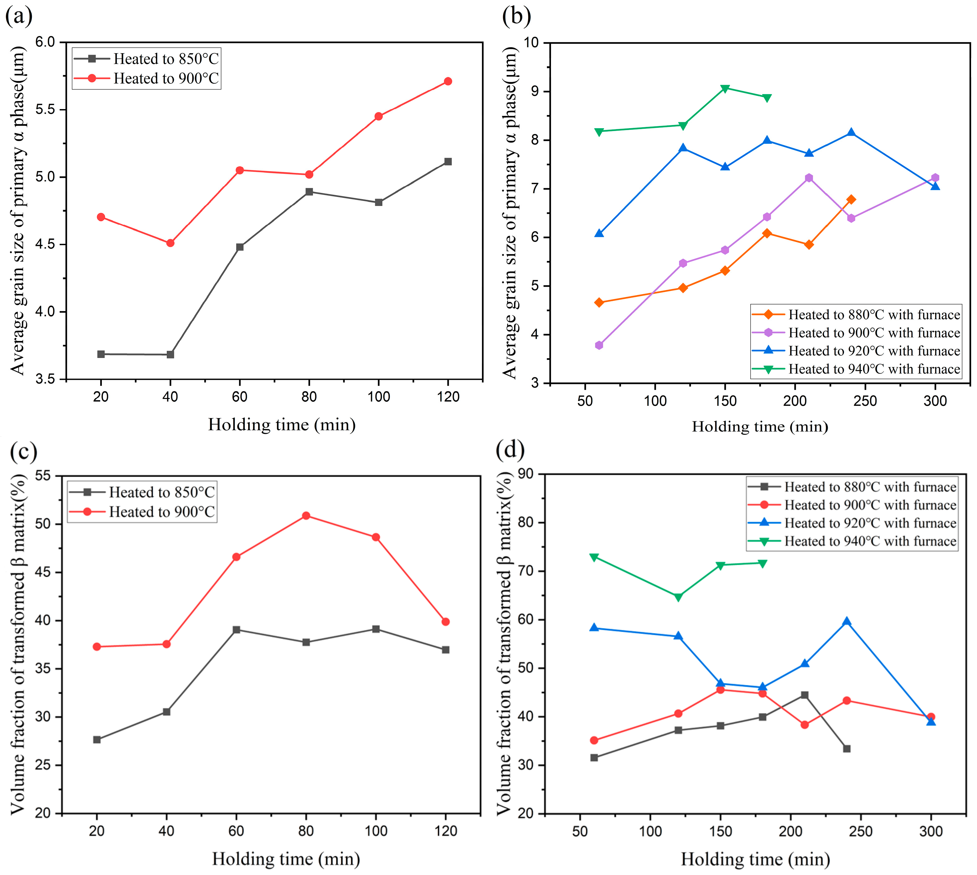
The relationship between the average grain size of the primary α phase and the volume fraction of the transformed β matrix with the holding temperature and holding time is presented in the form of pictures and analyzed. With the same holding time but different holding temperatures, the average grain size of the primary α phase tends to increase with an increasing holding temperature, as shown in Figure 4a,b, while the volume fraction of the transformed β matrix as a whole also tends to increase, as shown in Figure 4c,d. In the case of the same holding time and different holding temperatures, the average grain size of the primary α phase shows an overall trend of increasing with the increase in the holding time, as shown in Figure 4a,b, while the volume fraction of the transformed β matrix shows an overall trend of first increasing and then decreasing, as shown in Figure 4c,d. The volume fraction of the transformed β matrix decreases when the holding time reaches about 210 min, probably due to the non-uniform distribution of the plate elements.

3.3. Signal Processing and Longitudinal Wave Velocity Extraction

The collected laser ultrasound signal often has a large amount of noise, which makes the location of the lowest point for finding the longitudinal wave trough not unique, thus causing the time difference between the two wave peaks to be inaccurate. As a result, a signal noise reduction processing method is needed to improve the effectiveness and reliability of the laser ultrasound detection system. In this paper, we use variational modal decomposition (VMD) denoising, which considers that any signal is a superposition of subsignals with dominance of different frequencies. This transforms the signal processing problem into a variational model solving problem and determines the center frequency and bandwidth of each mode by iteratively searching the extrema of the variational model, thus decomposing the noise-bearing signal into a series of band-limited intrinsic mode functions (BLIMFs) with sparsity and finite bandwidth [36]. Then, the longitudinal ultrasound signal with a specific structure is selected for reconstruction according to the IMF function after the decomposition of the center frequency. The results of the reconstructed ultrasound signal are shown in Figure 5.
In this paper, the laser ultrasonic inspection system is used to receive the ultrasonic waves from the opposite side. That is, the time difference between the two adjacent peaks of ultrasound represents the distance of the ultrasound propagation of twice the thickness. Therefore, the longitudinal wave velocity of the ultrasonic waves can be obtained with Equation (1).
v = 2 d t i t i 1
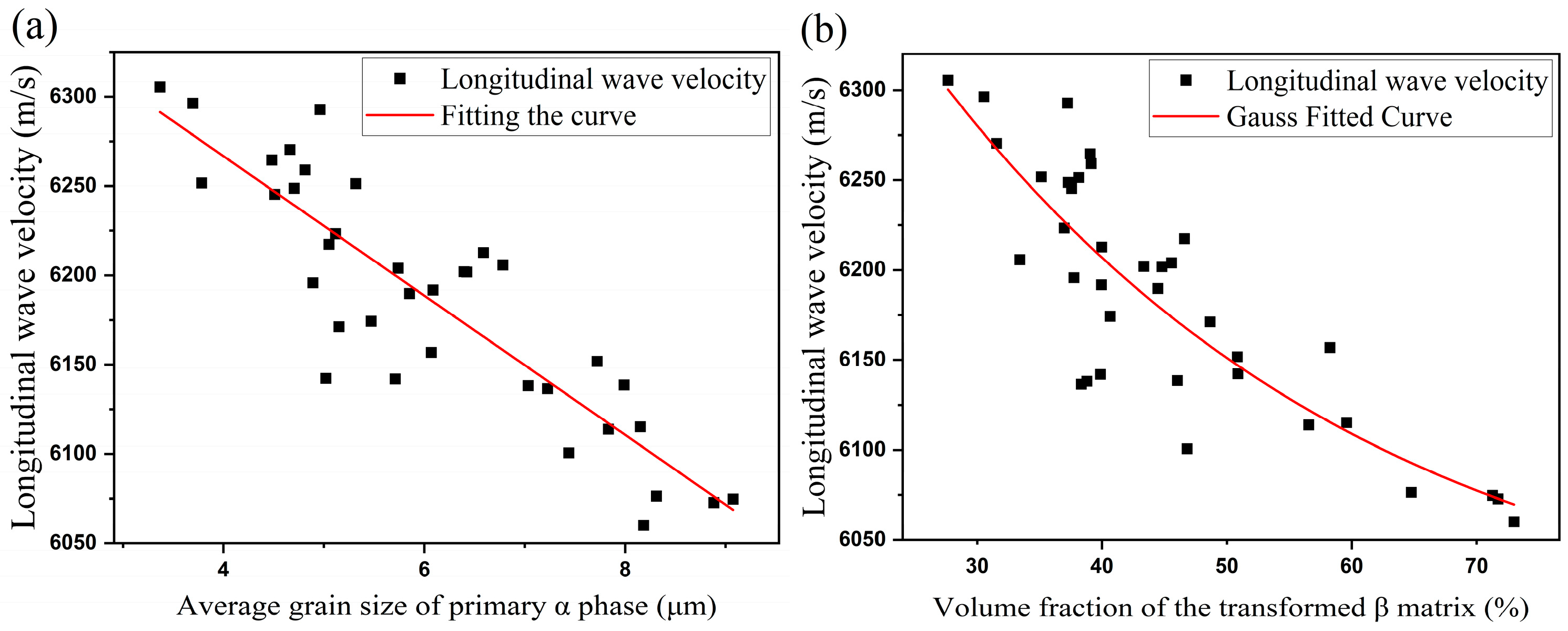
where d is the thickness of the specimen and t is the time at the wave crest. The velocities during the propagation of every two adjacent echoes from the second to the sixth echo were obtained, and the four velocity averages were obtained (in order to facilitate the discussion of the relationship between the longitudinal wave velocities and the microstructure of the titanium alloy). The polynomial equation was used to fit the relationship between the longitudinal wave velocity and the average grain size of the primary α phase, and the fitted graph shown in Figure 6a was obtained, from which it can be seen that the longitudinal wave velocity shows a linear decrease with the increase in the average grain size of the primary α phase. The Gaussian equation was used to fit the relationship between the longitudinal wave velocity and the volume fraction of the transformed β matrix, and the fitted plot shown in Figure 6b was obtained, from which it can be seen that the longitudinal wave velocity also shows a decreasing trend as the volume fraction of the transformed β matrix increases.

4. Analysis and Discussion

4.1. RFR Model Building

Random forest regression (RFR) is an algorithm that integrates multiple trees based on the idea of Bagging in integration learning. The basic unit is the regression tree. For the regression problem in this paper, each decision tree is a regressor, and, in the training phase, the random forest uses bootstrap sampling to collect several different subtraining sets from the input training dataset to train different binomial regression trees in turn. The feature subspace of each split node is randomly drawn from the total feature space when training the regression decision tree, and then the optimal features are selected for splitting within it, according to the principle of the minimum mean squared error. That is, for each input sample, there will be N trees with N regression results. This approach not only ensures the randomness and independence between trees, thus reducing the degree of overfitting, but also increases the robustness and stability of the final model prediction results. In the prediction phase, the random forest averages the predictions of the internal N decision trees to obtain the final output, a mechanism that greatly improves the prediction accuracy of the model.
The random forest regression algorithm process is as follows. (1) Using the Bagging idea, a subset k of the training samples of size N is generated by randomly putting back a sampling of the original training set. (2) A single regression decision tree is constructed by randomly selecting m features (m < M) among M feature attributes and performing node splitting. (3) Steps (1) and (2) are repeated to construct the multiple regression decision trees, so that each decision tree grows maximally to form a decision forest. (4) The prediction values of all the decision trees are averaged to obtain the final prediction results. The algorithm flow is shown in Figure 7.

4.2. Construction and Validation Results of RFR Model

The velocity of every two adjacent echoes in the signal should theoretically be the same, but the actual velocity is not equal, and it is known that there is a high correlation between the average grain size of the primary α phase and the longitudinal wave velocity. Therefore, the four longitudinal velocities of the ultrasonic signal were used as the input features (as shown in Table 3), and the average grain size of the primary α phase was used as the output. The average grain size prediction model of the incipient α-phase was constructed using the random forest regression to achieve the prediction of the average grain size of the primary α phase. Similarly, a prediction model of the volume fraction of the transformed β matrix can be constructed using the random forest regression to achieve the prediction of the volume fraction of the transformed β matrix.
The total number of samples in the above experiments was 36. Eight experiments were conducted for each sample, and a total of 288 sets of data were obtained as the total sample size. The sample data were divided into a training set and a test set according to a ratio of 30:6, where the training set was used to train and optimize the parameters of the model and the test set was used to evaluate the final prediction accuracy of the model. The number of training set samples was 240 data sets and the test set samples were 48 data sets. The prediction models for the average grain size of the primary α phase and the volume fraction of the transformed β matrix were constructed based on the above random forest regression principle. To exclude the phenomenon of model sub-optimization caused by unreasonable model parameter settings, the mean square error (MSE) was used as the scoring index for the parameter search, prior to the model training and evaluation, to determine the number of trees and leaf nodes of the decision tree of the RFR model. The higher the number of decision trees among the main parameters of the model, the better the training effect, and the smaller the mean square error means the better the prediction ability of the model. The expression is calculated as follows:
M S E = 1 m i = 1 m y i y ^ i 2
where M S E is the mean square error; y ^ i and y i are the predicted and actual values of the ith sample; and m is the sample size of the corresponding sample.
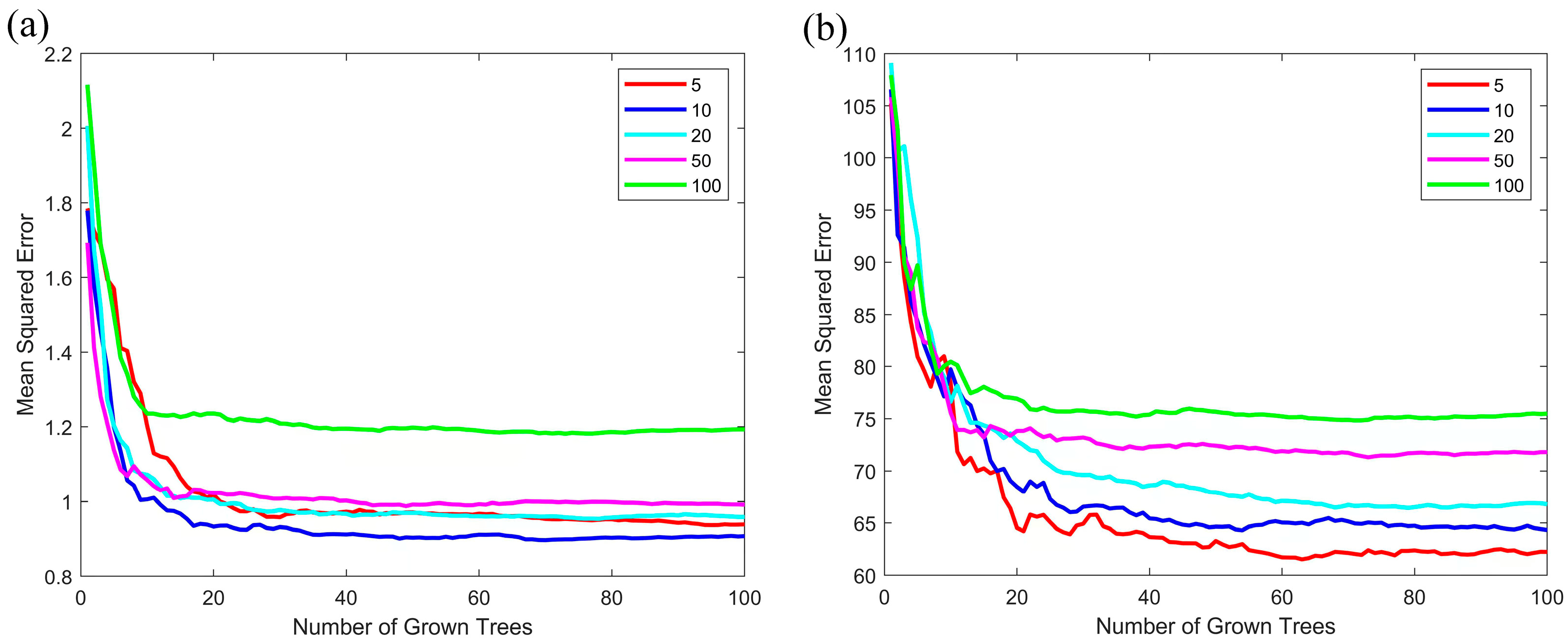
For the prediction model of the average grain size of the primary α phase, as shown in Figure 8a, the model converges and the value of the MSE is minimized when the number of decision trees is 100 and the number of leaf nodes is 10. As a result, the number of decision trees was set to 100 and the number of leaf nodes was set to 10. Similarly, for the prediction model of the volume fraction of the transformed β matrix, as shown in Figure 8b, the model converges and the value of MSE is minimized when the tree is 100 and when the number of leaf nodes is 5. Therefore, the number of decision trees was set to 100 and the number of leaf nodes was set to 5.
When the optimal parameters of the model were determined, the root mean square error (RMSE), the squared absolute value error (MAE), and the coefficient of determination (R2) were used as measures of how well the model results fitted the actual values, in order to quantitatively analyze and compare the prediction results of the model. When the RMSE and MAE are smaller, the closer R2 is to 1, the better the model fitting effect and the higher the accuracy. The calculation method is as follows.
R 2 = 1 i = 1 m y ^ i y i 2 i = 1 m y i y ¯ 2
R M S E = i = 1 m y ^ i y i 2 m
M A E = 1 m i = 1 m y ^ i y i
where y ^ i and y i are the predicted and actual values of the ith sample, respectively; y ¯ is the average of the actual values of the samples; and m is the sample capacity of the corresponding sample. The test set was brought into the two trained models separately, and the coefficients of determination R2 and the RMSE and MAE of the models were calculated as shown in Table 4.
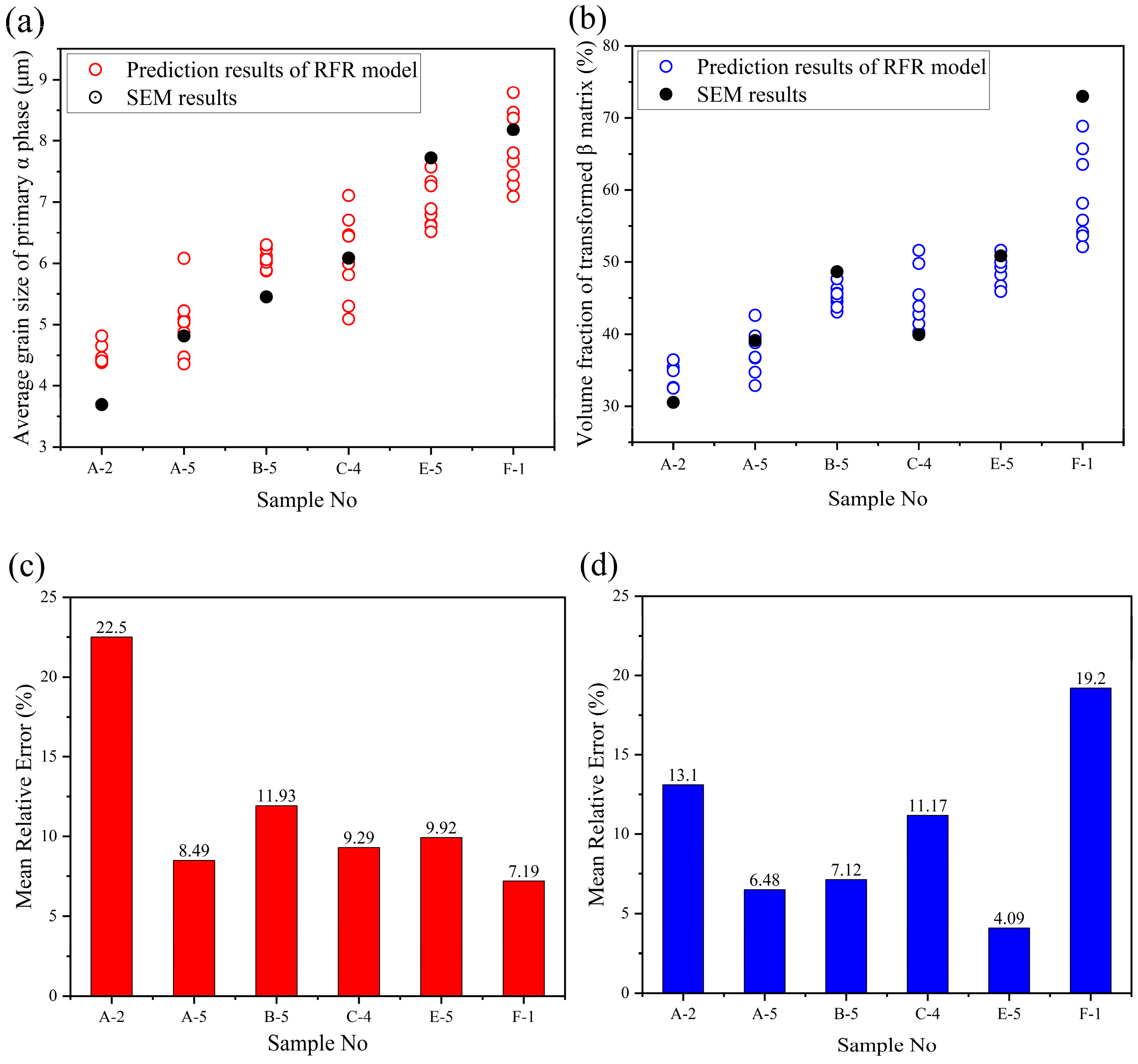
As can be seen from Table 4, the R2 of the models are 0.82 and 0.77, respectively, indicating that both of the established RFR models fit relatively well. In addition, the predicted values and SEM results of the two RFR models were visualized for a more intuitive understanding of the models’ predictions. For the prediction model of the average grain of the primary α phase, as shown in Figure 9a, each specimen has one SEM result marked as a black solid circle and eight predicted results marked as red hollow circles. For the prediction model of the transformed β matrix volume fraction, as shown in Figure 9b, each specimen has one SEM result marked as a black solid circle and eight predicted results marked as blue hollow circles. The mean relative errors between the predicted and SEM results were calculated for each specimen in the two models. In the prediction model for the average grain size of the primary α phase, the mean relative errors of the prediction results for specimens #A-2, #A-5, #B-5, #C-4, #E-5, and #F-1 were 22.5%, 8.49%, 11.93%, 9.29%, 9.92%, and 7.19%, respectively, as shown in Figure 9c. In the prediction model for the volume fraction of the transformed β matrix, the mean relative errors of the prediction results for specimens #A-2, #A-5, #B-5, #C-4, #E-5, and #F-1 were 13.1%, 6.48%, 7.12%, 11.17%, 4.09%, and 19.2%, respectively, as shown in Figure 9d. The mean values of the mean relative errors of the predicted mean grain size of the native α phase and the volume fraction of the transformed β matrix for the six samples in the two prediction models were 11.55% and 10.19%, respectively, and the RMSE and MAE obtained from both prediction models were relatively small, as shown in Table 4, indicating that the two established RFR models have a high prediction accuracy.
In addition, it can be seen from Figure 9c,d that the prediction results for specimens A-2 and F-1 deviate significantly. This is because, in the regression problem, the prediction range that can be performed by the random forest is constrained by the highest and lowest parameters in the training data, and its prediction effect is based on the existing experience. The average grain size of the primary α phase of specimen A-2 and the volume fraction of the transformed β matrix of specimen F-1 are outside the training set, so the prediction results of these two specimens are poorer in the prediction model.

5. Conclusions

In this paper, a Ti-6Al-4V titanium alloy with a different microstructure is taken as the research object. Based on laser ultrasonic detection technology, the VMD signal processing method, and a machine learning algorithm, the influence of the primary α phase volume fraction of theTi-6Al-4V titanium alloy on the ultrasonic sound velocity is studied. The primary α phase volume fraction is predicted by the support vector machine and random forest regression algorithm. The conclusion is as follows:
(1) The variation mode decomposition algorithm is suitable for processing nonlinear and non-stationary signals, such as laser ultrasonic signals. After processing the laser ultrasonic signal, the high-frequency noise contained in the signal and the baseline drift caused by low-frequency vibration and thermal expansion are effectively filtered out, and the signal-to-noise ratio is obviously improved. The relationship between the primary α phase volume fraction and the ultrasonic signal velocity of the Ti-6Al-4V titanium alloy was established by fitting the polynomial equation. It was found that the relationship between the primary α phase volume fraction and the ultrasonic sound velocity was linear, and the ultrasonic sound velocity increased with the increase in the primary α volume fraction.
(2) Based on the support vector machine algorithm and random forest regression algorithm, the prediction model of the primary α phase volume fraction of the Ti-6Al-4V titanium alloy was established with four sound velocities of each ultrasonic signal obtained by laser ultrasonic detection as the input variables and the primary α phase volume fraction of the Ti-6Al-4V titanium alloy as the output variable. The data of forty samples from five samples in the two model test sets were inputted into the model for prediction, and the prediction results of each sample were obtained. The evaluation indices R2, RMSE, and MAE of the SVM prediction results were 0.840, 4.119, and 3.651, respectively, and the average relative error of the prediction results of the five samples was 6.71%. The evaluation indices R2, RMSE, and MAE of the random forest regression prediction results were 0.871, 3.993, and 3.406, respectively, and the average relative error of the prediction results of the five samples was 6.36%, indicating that the two models had a good prediction accuracy and that the two models could better predict the primary α phase volume fraction. The random forest regression model has a higher prediction accuracy, but the prediction stability is relatively low for small samples, while the support vector machine prediction model has a better stability for small samples. The two methods can be selected or combined according to different conditions to improve the characterization accuracy of the ultrasonic microstructure.

Author Contributions

Conceptualization, J.W. and A.Y.; methodology, S.Y.; software, Y.H.; data curation, X.W., H.C., C.Y. and F.H.; writing—original draft preparation, J.W.; writing—review and editing, A.Y.; supervision, A.Y.; and funding acquisition, J.W. and A.Y. All authors have read and agreed to the published version of this manuscript.

Funding

This project was supported by the Natural Science Foundation of Zhejiang Provence (Y24E050035) and Projects in Science and Technique Plans of Ningbo City (2023Z012).

Data Availability Statement

The data presented in this study are available on request from the corresponding author.

Conflicts of Interest

Author J.W., S.Y., X.W., H.C., F.H. and C.Y. were employed by the company CGN Inspection Technology Co., Ltd. The remaining authors declare that the research was conducted in the absence of any commercial or financial relationships that could be construed as a potential conflict of interest.

References

  1. Cui, C.; Hu, B.; Zhao, L.; Liu, S. Titanium alloy production technology, market prospects and industry development. Mater. Design 2011, 32, 1684–1691. [Google Scholar] [CrossRef]
  2. Sun, L.; Li, M.; Li, H. Dynamic Recrystallization-Related Interface Phase Boundary Migration of TC17/TC4 Bond with Initial Equiaxed Microstructure. J. Nutr. 2019, 71, 2253–2261. [Google Scholar] [CrossRef]
  3. Yu, Z.; Yu, S.; Cheng, J.; Ma, X. Development and Application of Novel Biomedical Titanium Alloy Materials. Acta Metall. Sin. 2017, 53, 1238–1264. [Google Scholar]
  4. Chong, Y.; Bhattacharjee, T.; Tsuji, N. Bi-lamellar microstructure in Ti–6Al–4V: Microstructure evolution and mechanical properties. Mat. Sci. Eng. A 2019, 762, 138077. [Google Scholar] [CrossRef]
  5. Long, W.; Zhang, S.; Liang, Y.-L.; Ou, M.-G. Influence of multi-stage heat treatment on the microstructure and mechanical properties of TC21 titanium alloy. Int. J. Min. Met. Mater. 2021, 28, 296–304. [Google Scholar] [CrossRef]
  6. Mandal, P.K.; Mathews, M.S.; A Daniel, B.; Devasia, J. Effect of ageing treatment on microstructure and mechanical properties of α + β type titanium alloy used for biomaterials. IOP Conf. Ser. Mater. Sci. Eng. 2019, 561, 012060. [Google Scholar] [CrossRef]
  7. Zhao, P.; Wei, C.; Li, Y.; Tao, J.; Zhang, C.; Xiao, X.; Zhang, M. Effect of heat treatment on the microstructure, microhardness and impact toughness of TC11 and TC17 linear friction welded joint. Mat. Sci. Eng. A 2021, 803, 140496. [Google Scholar] [CrossRef]
  8. Roman, I.; Ward, C.H. Acoustic-Emission Characterization of the Deformation and Fracture of A Ti3Al Alloy. Scripta Mater. 1992, 27, 413–418. [Google Scholar] [CrossRef]
  9. Chen, G.; Liu, C. Cyclic Plastic Deformation Behavior of TC4 Titanium Alloy Under Different Microstructures and Load Conditions Using Finite Element Method. J. Fail. Anal. Prev. 2021, 21, 678–688. [Google Scholar] [CrossRef]
  10. Maalekian, M.; Radis, R.; Militzer, M.; Moreau, A.; Poole, W. In situ measurement and modelling of austenite grain growth in a Ti/Nb microalloyed steel. Acta Mater. 2012, 60, 1015–1026. [Google Scholar] [CrossRef]
  11. Rodrigues, M.C.; Garcin, T.; Militzer, M. In-situ measurement of α formation kinetics in a metastable β Ti-5553 alloy using laser ultrasonics. J. Alloys Compd. 2021, 866, 158954. [Google Scholar] [CrossRef]
  12. Li, Y.; Hou, S.; Chai, Y.; Zhou, Y.; Zou, Y. Nondestructive measurement of the grain size of laser cladding coatings using a laser ultrasonic method. Appl. Opt. 2022, 61, 1885–1891. [Google Scholar] [CrossRef] [PubMed]
  13. Keyvani, M.; Garcin, T.; Militzer, M.; Fabregue, D. Laser ultrasonic measurement of recrystallization and grain growth in an L605 cobalt superalloy. Mater. Charact. 2020, 167, 110465. [Google Scholar] [CrossRef]
  14. Falkenström, M.; Engman, M.; Lindh-Ulmgren, E.; Hutchinson, B. Laser ultrasonics for process control in the metal industry. Nondestruct. Test. Eval. 2011, 26, 237–252. [Google Scholar] [CrossRef]
  15. Du, H.; Turner, J.A. Ultrasonic attenuation in pearlitic steel. Ultrasonics 2014, 54, 882–887. [Google Scholar] [CrossRef] [PubMed]
  16. Dong, F.; Wang, X.; Yang, Q.; Liu, H.; Xu, D.; Sun, Y.; Zhang, Y.; Xue, R.; Krishnaswamy, S. In-situ measurement of Ti-6Al-4V grain size distribution using laser-ultrasonic technique. Scr. Mater. 2018, 154, 40–44. [Google Scholar] [CrossRef]
  17. White, R.M. Generation of elastic waves by transient surface heating. J. Appl. Phys. 1963, 34, 3559–3567. [Google Scholar] [CrossRef]
  18. Moreau, A.; Lévesque, D.; Lord, M.; Dubois, M.; Monchalin, J.-P.; Padioleau, C.; Bussière, J. On-line measurement of texture, thickness and plastic strain ratio using laser-ultrasound resonance spectroscopy. Ultrasonics 2002, 40, 1047–1056. [Google Scholar] [CrossRef]
  19. Kruger, S.E.; Damm, E.B. Monitoring austenite decomposition by ultrasonic velocity. Mat. Sci. Eng. A 2006, 425, 238–243. [Google Scholar] [CrossRef]
  20. Shinbine, A.; Garcin, T.; Sinclair, C. In-situ laser ultrasonic measurement of the hcp to bcc transformation in commercially pure titanium. Mater. Charact. 2016, 117, 57–64. [Google Scholar] [CrossRef]
  21. Sarpun, I.H.; Selami, K.M.; Tuncel, S. Mean grain size determination in marbles by ultrasonic velocity techniques. NDT&E Int. 2005, 38, 21–25. [Google Scholar]
  22. Li, P.; Chu, S.; Chou, C.; Chen, F. Use of ultrasonic velocity for nondestructive evaluation of ferrite content in duplex Fe-Mn-Al alloy steels. Scr. Metall. Mater. 1992, 26, 127–132. [Google Scholar] [CrossRef]
  23. Palanichamy, P.; Joseph, A.; Jayakumar, T.; Raj, B. Ultrasonic velocity measurements for estimation of grain size in austenitic stainless steel. NDT&E Int. 1995, 28, 179–185. [Google Scholar]
  24. Gronau, O.; Regener, D. Ultrasonic testing of extruded and rolled green compacts from TiAl. NDT&E Int. 1997, 30, 351–357. [Google Scholar]
  25. Senkov, O.N.; Dubois, M.; Jonas, J.J. Elastic moduli of titanium-hydrogen alloys in the temperature range 20 degrees C to 1100 degrees C. Metall. Mater. Trans. B 1996, 27, 3963–3970. [Google Scholar] [CrossRef]
  26. Ünal, R.; Sarpün, I.H.; Yalım, H.A.; Erol, A.; Özdemir, T.; Tuncel, S. The mean grain size determination of boron carbide (B4C)-aluminium (Al) and boron carbide (B4C)-nickel (Ni) composites by ultrasonic velocity technique. Mater. Charact. 2006, 56, 241–244. [Google Scholar] [CrossRef]
  27. Yin, A.; Yang, Q.; He, F.; Wang, X.; Dong, F.; Wang, Y.; Shu, X. Laser ultrasound-based nondestructive inspection method for average grain size of mild steel. Chin. J. Mech. Eng-En. 2017, 53, 9. (In Chinese) [Google Scholar]
  28. Bate, P.; Lundin, P.; Lindh-Ulmgren, E.; Hutchinson, B. Application of laser-ultrasonics to texture measurements in metal processing. Acta Mater. 2017, 123, 329–336. [Google Scholar] [CrossRef]
  29. Zhang, J.; Wang, X.; Xu, D.; Yang, Q.; Zhao, J.; Xue, R. Prediction of volume fraction of primary α phase in dual-phase titanium alloy based on laser ultrasonic. Measurement 2022, 195, 111115. [Google Scholar] [CrossRef]
  30. Chen, C.; Zhang, X. Research on laser ultrasonic surface defect identification based on a support vector machine. Sci. Prog.-Uk 2021, 104, 00368504211059038. [Google Scholar] [CrossRef]
  31. Taylor, P.L.; Conduit, G. Machine learning predictions of superalloy microstructure. Comp. Mater. Sci. 2022, 201, 110916. [Google Scholar] [CrossRef]
  32. Jin, Y.; Zhao, J.; Zhang, C.; Luo, J.; Wang, S. Research on Neural Network Prediction of Multidirectional Forging Microstructure Evolution of GH4169 Superalloy. J. Mater. Eng. Perform. 2021, 30, 2708–2719. [Google Scholar] [CrossRef]
  33. Luo, J.H.; Liu, X.F.; Shi, Z.Z.; Liu, Y.F. Microstructure quantification of Cu–4.7 Sn alloys prepared by two-phase zone continuous casting and a BP artificial neural network model for microstructure prediction. Rare Metals 2019, 38, 1124–1130. [Google Scholar] [CrossRef]
  34. Xue, R.; Wang, X.; Yang, Q.; Xu, D.; Sun, Y.; Zhang, J.; Krishnaswamy, S. Grain size distribution characterization of aluminum with a particle swarm optimization neural network using laser ultrasonics. Appl. Acoust. 2021, 180, 108125. [Google Scholar] [CrossRef]
  35. Zhang, J.; Yin, A.; Tao, C.; Wang, Y.; Zhu, Z.; Peng, H.; Shu, X. Rapid measurement of the fourth-order texture coefficient by laser ultrasonic surface acoustic waves based on a neural network expert system. Appl. Opt. 2019, 58, 626–634. [Google Scholar] [CrossRef]
  36. Dragomiretskiy, K.; Zosso, D. Variational mode decomposition. IEEE T Signal Proces. 2013, 62, 531–544. [Google Scholar] [CrossRef]
Figure 1. Laser ultrasonic detection system. (a) Experimental device diagram of laser ultrasonic detection system; and (b) schematic diagram of laser ultrasonic detection system.
Crystals 14 00607 g001
Figure 2. Microstructure diagram of the bistatic tissue: (a) sample #A-6; (b) sample #B-6; (c) sample #C-2; (d) sample #D-2; (e) sample #E-2; and (f) sample #F-2.
Crystals 14 00607 g002
Figure 3. Diagram of the software processing. (a) Denoised map; (b) flip diagram; and (c) binarization diagram.
Crystals 14 00607 g003
Figure 4. The average grain size of the primary α phase and the volume fraction of the transformed β matrix of the samples at different holding temperatures and holding times are shown: (a) the primary α phase grain size of sample groups #A and #B; (b) the primary α phase grain size of sample groups #C, #D, #E, and #F; (c) the volume fraction of the transformed β matrix of sample groups #A and #B; and (d) the volume fraction of the transformed β matrix of sample groups #C, #D, #E, and #F.
Crystals 14 00607 g004
Figure 5. Original and reconstructed signals.
Crystals 14 00607 g005
Figure 6. Fitting of longitudinal wave velocity and microstructure parameters: (a) the longitudinal wave velocity and the average grain size of the primary α phase; and (b) the longitudinal wave velocity and the volume fraction of the transformed β matrix.
Crystals 14 00607 g006
Figure 7. Calculation flow of the random forest regression algorithm.
Crystals 14 00607 g007
Figure 8. Optimization process of RFR model parameters: (a) prediction model for the average grain size of the primary α phase; and (b) prediction model for the volume fraction of the transformed β matrix.
Crystals 14 00607 g008
Figure 9. RFR model prediction results and mean relative error. (a) Prediction results of the average grain size of the primary α phase; (b) prediction results of the volume fraction of the transformed β matrix; (c) mean relative error in the prediction of the average grain size of the primary α phase; and (d) mean relative error in the prediction of the volume fraction of the transformed β matrix.
Crystals 14 00607 g009
Table 1. Chemical composition of Ti-6Al-4V for experiment.
ElementTiFeAlVHCON
Content/%Remaining0.04956.07644.09200.00420.01130.12480.0192
Table 2. Ti-6Al-4V heat treatment process.
Group NumberHolding Temperature/°CHolding Time/minCooling Method
AHeated to 850 °C20/40/60/80/100/120Air cooling
BHeated to 900 °C20/40/60/80/100/120
CHeated to 880 °C with furnace60/120/150/180/210/240
DHeated to 900 °C with furnace60/120/150/180/210/240/300
EHeated to 920 °C with furnace60/120/150/180/210/240/300
FHeated to 940 °C with furnace60/120/150/180
Table 3. Input parameters of the RFR model.
Ultrasonic Parameters
P 1 = v 1
P 2 = v 2
P 3 = v 3
P 4 = v 4
Table 4. RFR model evaluation indicators.
ModelTest Set
R2RMSEMAE
Average grain size prediction model0.820.71400.6414
Volume fraction prediction model0.777.60645.2933
Disclaimer/Publisher’s Note: The statements, opinions and data contained in all publications are solely those of the individual author(s) and contributor(s) and not of MDPI and/or the editor(s). MDPI and/or the editor(s) disclaim responsibility for any injury to people or property resulting from any ideas, methods, instructions or products referred to in the content.