Magnon Confinement on the Two-Dimensional Penrose Lattice: Perpendicular-Space Analysis of the Dynamic Structure Factor

Abstract

Employing the spin-wave formalism within and beyond the harmonic-oscillator approx-imation, we study the dynamic structure factors of spin-${\displaystyle \frac{1}{2}}$ nearest-neighbor quantum Heisenberg antiferromagnets on two-dimensional quasiperiodic lattices with particular emphasis on a mag-netic analog to the well-known confined states of a hopping Hamiltonian for independent electrons on a two-dimensional Penrose lattice. We present comprehensive calculations on the C_5v Penrose tiling in comparison with the C_8v Ammann–Beenker tiling, revealing their decagonal and octagonal antiferromagnetic microstructures. Their dynamic spin structure factors both exhibit linear soft modes emergent at magnetic Bragg wavevectors and have nearly or fairly flat scattering bands, signifying magnetic excitations localized in some way, at several different energies in a self-similar manner. In particular, the lowest-lying highly flat mode is distinctive of the Penrose lattice, which is mediated by its unique antiferromagnons confined within tricoordinated sites only, unlike their itinerant electron counterparts involving pentacoordinated, as well as tricoordinated, sites. Bringing harmonic antiferromagnons into higher-order quantum interaction splits, the lowest-lying nearly flat scattering band in two, each mediated by further confined antiferromagnons, which is fully demonstrated and throughly visualized in the perpendicular as well as real spaces. We disclose superconfined antiferromagnons on the two-dimensional Penrose lattice.

1. Introduction

In 1974, Penrose [1] discovered an extreme manner of non-periodic tiling in two dimensions (Figure 1a). What we call the Penrose lattice consists of two rhombi with angles of ${\displaystyle \frac{\pi }{5}}$ and ${\displaystyle \frac{2\pi }{5}}$ laid out with a matching rule but without any translational symmetry (Figure 1b). The Penrose lattice has a crystallographically forbidden five-fold rotational symmetry and a self-similar structure characterized by the golden ratio ${\displaystyle \frac{1+\sqrt{5}}{2}}$ [2]. The diffraction pattern of the Penrose lattice, however, consists of sharp $\delta$-function peaks [3]. Hence, it follows that the Penrose lattice has a long-range positional order, which we nowadays refer to as “quasiperiodicity”. Besides the Penrose tile pattern, numerous ways of quasiperiodic tiling have been proposed to date, with eight-fold [4] and twelve-fold [5] rotational symmetries, for instance. Such unconventional geometries fascinate physicists as well as mathematicians. Several authors took their early interest in tight-binding models [6,7,8,9] on the Penrose lattice. When electrons hop on the vertices of each rhombus, they yield a macroscopically degenerate eigenlevel of zero energy in the thermodynamic limit [10,11,12]. While wavefunctions of these unique states are all strictly confined in a finite region, they take on a critical character, i.e., they are neither localized nor extended in the conventional sense to have no absolute length scale. The density of states consists of spiky bands and, in particular, the zero-energy confined states constitute a $\delta$-function peak, being isolated from all the rest by a gap of about one-tenth of the hopping energy t. All these findings are consequent from the self-similarity of the Penrose lattice.

The synthesis of an aluminum–manganese alloy of icosahedral point group symmetry [15] surprised us in a different context. Indeed its novel rotational symmetry, inconsistent with any translational symmetry, is suggestive of quasiperiodic tiling, but it was left out of solids before arguing whether this should also come under crystals, due to its lack of thermodynamic stability. However, thermodynamically stable quasicrystals [16,17] were synthesized a few years later, and it did not take much time until the concept and definition of “quasicrystals” [18,19] were established. The birth of quasicrystals caused a revolution in materials science, sparking a renewed interest in the Penrose lattice. Correlated electrons on the two-dimensional Penrose lattice have been investigated in terms of pure [20] and extended [21] Hubbard models. Without any Coulomb interaction, the ground-state charge distribution is uniform at half-band filling. Once the system deviates from its half filling, the charge distribution is no longer uniform, which is the consequence of various constituent coordination numbers z, ranging from 3 to 7. Coulomb interactions lift the degeneracy of the confined states and induce a magnetic or charge order. At half filling, an infinitesimal on-site Coulomb repulsion U induces nonzero local staggered magnetizations because of the macroscopically degenerate zero-energy states. With increasing U, the confined states come to constitute a band of width in proportion to U provided $U\ll t$. The intersite Coulomb repulsion V breaks the electron-hole symmetry and serves to induce charge inhomogeneity rather than any magnetic ordering. If we dope the system with holes or electrons, it becomes metallic with its confined states being totally vacant or fully occupied, and then its ground state is charge ordered in a nonuniform and self-similar manner.

In the strong-correlation limit, the half-filled single-band Hubbard model on an arbitrary lattice behaves as a spin-${\displaystyle \frac{1}{2}}$ Heisenberg antiferromagnet. Within the naivest spin-wave (SW) formalism, Wessel and Milat [22] calculated the dynamic structure factor, accessible to inelastic neutron scattering, of the nearest-neighbor antiferromagnetic spin-${\displaystyle \frac{1}{2}}$ Heisenberg model on the Ammann–Beenker octagonal tiling [4], which is another prominent example of a quasiperiodic lattice in two dimensions. They found linear soft modes near the magnetic Bragg peaks at low frequencies, self-similar structures at intermediate frequencies, and flat bands at high frequencies. These findings each are intriguing in themselves and more intriguing is their coexistence that has never happened in any conventional periodic system. The bipartiteness of two-dimensional quasiperiodic tilings such as the Penrose and Ammann–Beenker lattices allows quantum Monte Carlo simulations of antiferromagnetically exchange-coupled spins residing on them [23,24]. As in the case of the square-lattice antiferromagnet, they have Néel-ordered ground states, whose local staggered magnetizations; however, they vary site by site. The spatially averaged staggered magnetizations on the Penrose [23] and Ammann–Beenker [24] lattices are both larger than that on the square lattice [25], though they can be marked by the same coordination number $z=4$ on an average. This reads as the spatial inhomogeneity serving to reduce quantum fluctuations. The linear SW (LSW) theory well reproduces their bulk properties in general. Its estimates of the ground-state energy [22,23] are fairly accurate with an error less than 2 percent. The LSW theory securely guesses the ground-state staggered magnetizations as well when averaged spatially, but its findings for their local values each are no longer reliable quantitatively [22,26]. We must go beyond the harmonic-oscillator approximation in an attempt to reveal the very nature of quasiperiodic quantum magnets. Although the Penrose and Ammann–Beenker tilings have coordination numbers z ranging from 3 to 7 and 3 to 8, respectively, the former has more local environments (Figure 1c) and more complicated transformation rules than the latter. There may be differences as well as similarities between them, as was demonstrated in inelastic-light-scattering studies [27,28]. Thus motivated, we investigate static and dynamic spin structure factors for the nearest-neighbor antiferromagnetic spin-${\displaystyle \frac{1}{2}}$ Heisenberg model on the Penrose lattice, in comparison with those on the Ammann–Beenker lattice, in terms of the SW language within and beyond the harmonic-oscillator approximation.

The $3d$-transition-metal-based icosahedral quasicrystals such as Zn-Mg-Ho [29] and Zn-Mg-Tb [30] have extensively been studied through the use of neutron scattering [29,30,31] because their atomic structure is relatively well known and their sizable $4f$ magnetic moments are well localized and mostly isotropic. Recent technical progress of manipulating optical lattices [32,33,34] more and more motivate our theoretical investigations. Two-dimensional quasiperiodic optical potentials of five- [35] or eight-fold [36,37] rotational invariance were designed in terms of standing-wave lasers and consequent quasiperiodic long-range orders indeed manifested in sharp diffraction peaks [33,35]. By trapping ultracold bosonic or fermionic atoms in optical potentials and controlling the intensity, frequency, and polarization of the laser beam, we can change the on-site interaction and tunneling energy to obtain various effective spin Hamiltonians [38].

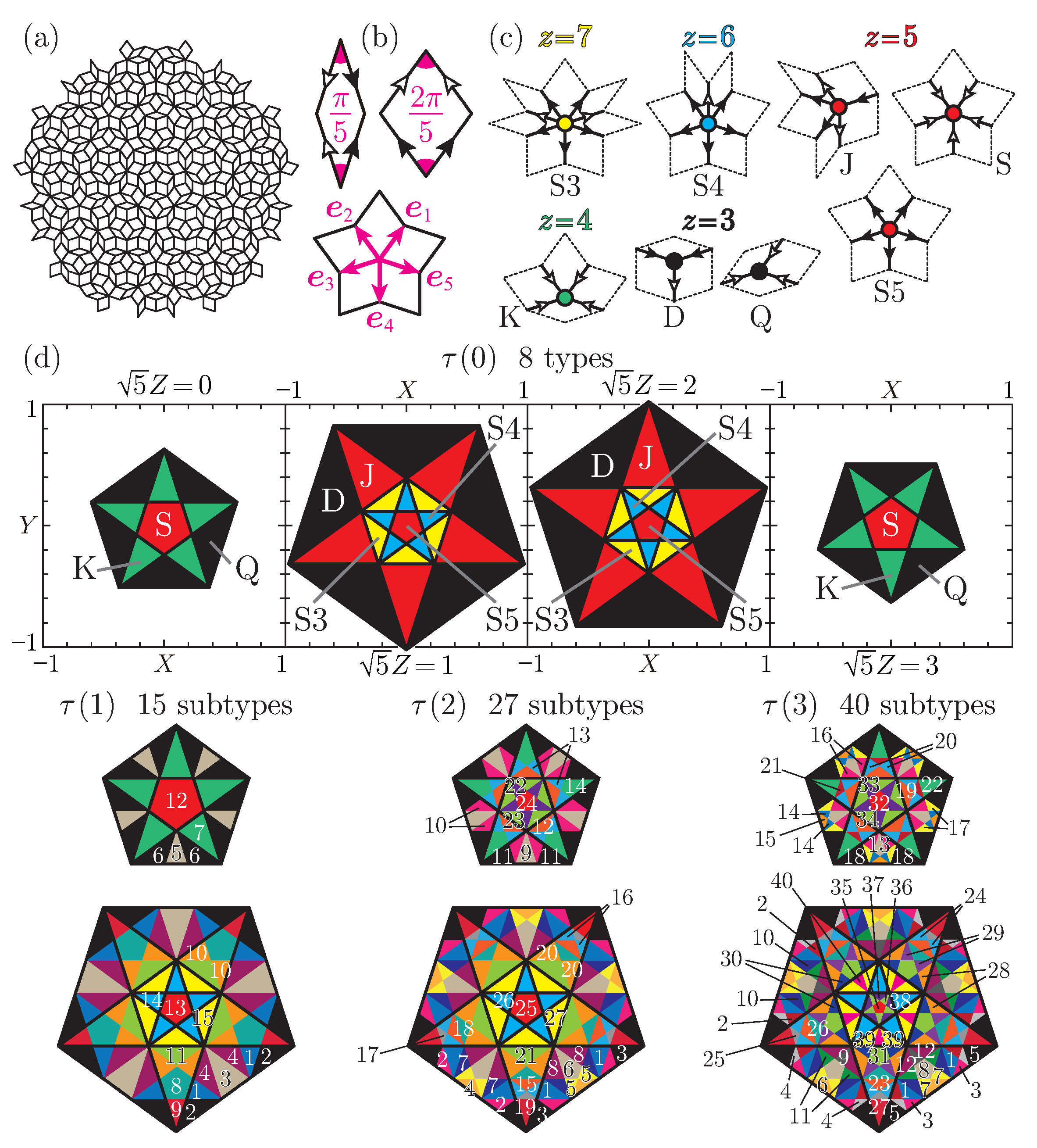
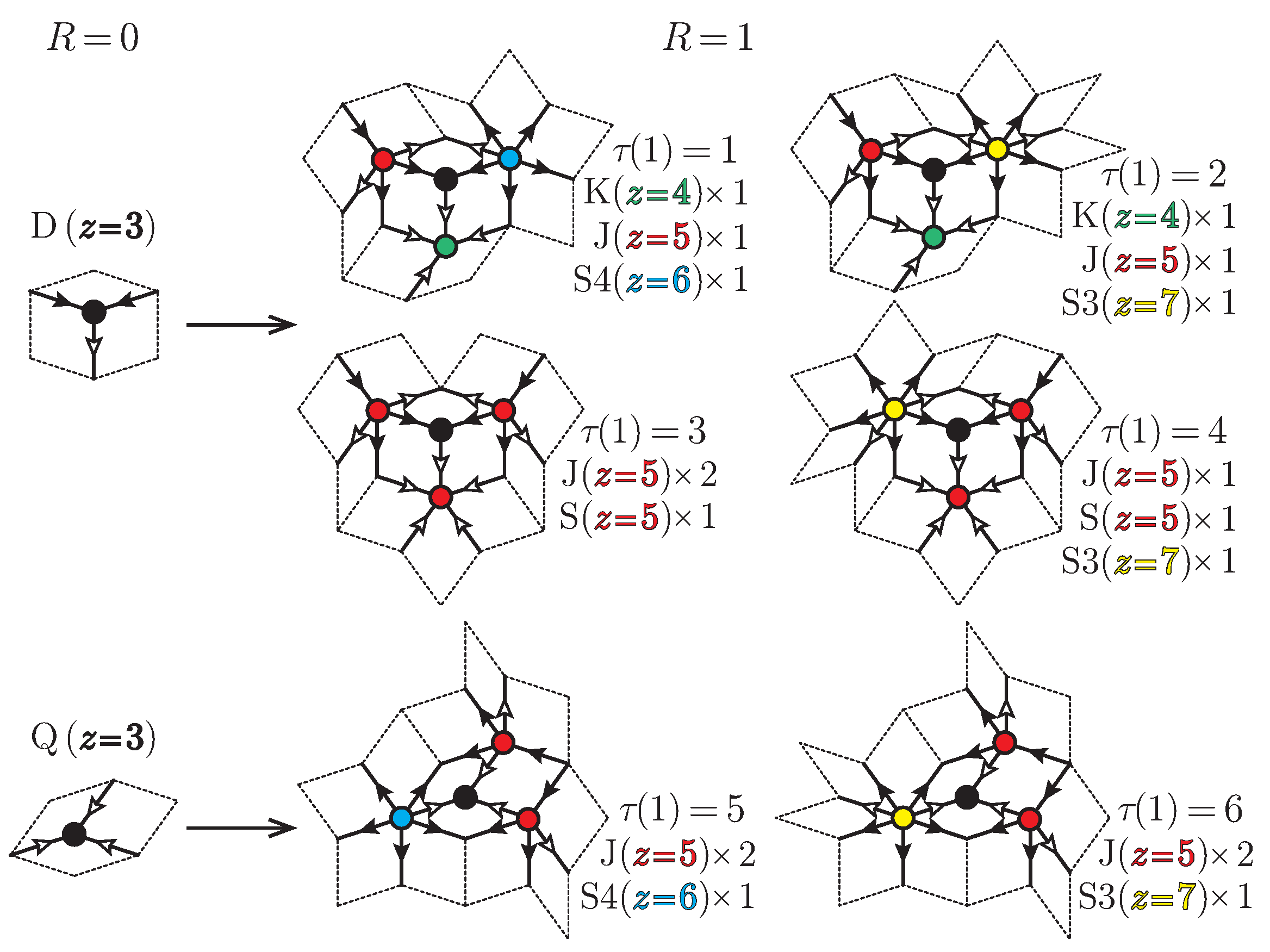
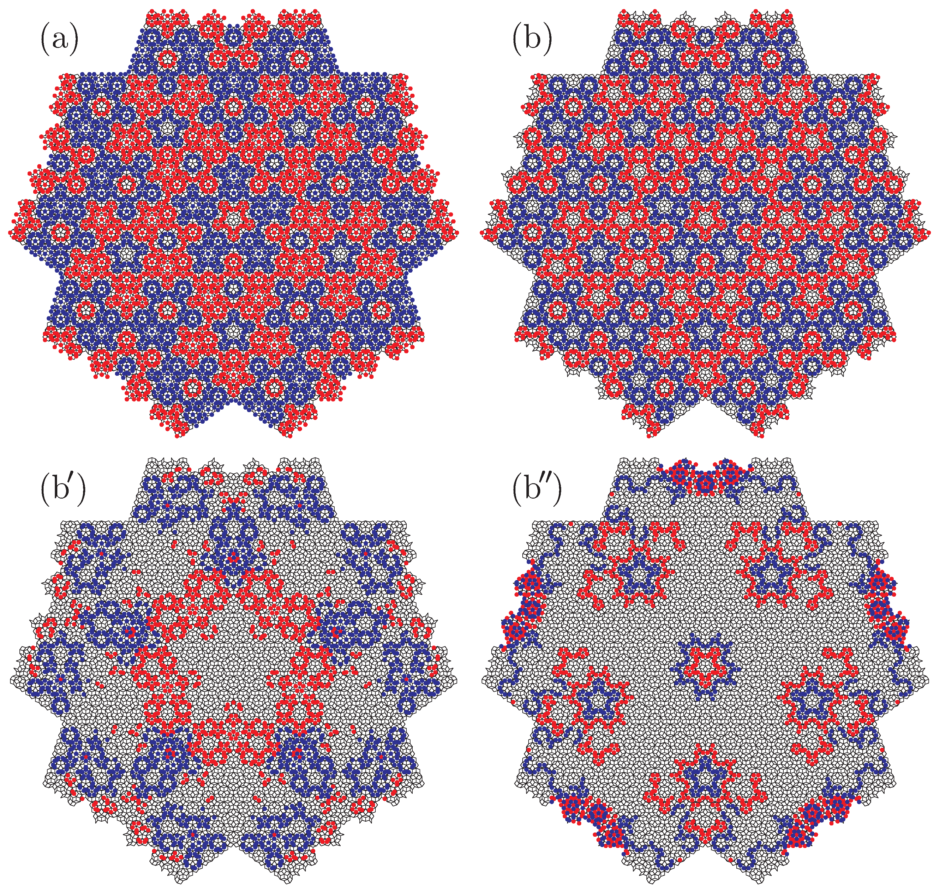
2. Quasiperiodic Tilings in Two Dimensions

Figure 1a is a Penrose lattice in two dimensions, which can be generated from minimal seeds (Figure 1b) by matching up their edges of the same arrow and repeating the inflation–deflation operation [20] with a magnification ratio of the golden number ${\displaystyle \frac{1+\sqrt{5}}{2}}$ to unity. Such operations yield the self-similarity of the Penrose lattice. Every two vertices on the Penrose lattice are connected by a linear combination of four independent primitive lattice vectors (Figure 1b) with a unique set of four integral coefficients. While the actual physical dimension d of the Penrose lattice equals 2, its indexing dimension or simply rank D amounts to 4 [39]. We can generally obtain a physically d-dimensional quasiperiodic tiling from a higher-than-d-dimensional periodic lattice through an algebraic approach [13,14]. The Penrose lattice is obtained as a projection of a five-dimensional hypercubic lattice onto a two-dimensional physical space,

$$\begin{array}{c}\hfill \left[\begin{array}{c}x\\ y\\ X\\ Y\\ Z\end{array}\right]=\sqrt{{\displaystyle \frac{2}{5}}}\left[\begin{array}{ccccc}cos{\varphi }_0& cos{\varphi }_1& cos{\varphi }_2& cos{\varphi }_3& cos{\varphi }_4\\ sin{\varphi }_0& sin{\varphi }_1& sin{\varphi }_2& sin{\varphi }_3& sin{\varphi }_4\\ cos{\varphi }_0& cos{\varphi }_2& cos{\varphi }_4& cos{\varphi }_6& cos{\varphi }_8\\ sin{\varphi }_0& sin{\varphi }_2& sin{\varphi }_4& sin{\varphi }_6& sin{\varphi }_8\\ {\displaystyle \frac{1}{\sqrt{2}}}& {\displaystyle \frac{1}{\sqrt{2}}}& {\displaystyle \frac{1}{\sqrt{2}}}& {\displaystyle \frac{1}{\sqrt{2}}}& {\displaystyle \frac{1}{\sqrt{2}}}\end{array}\right]\left[\begin{array}{c}{m}_1\\ m_2\\ m_3\\ m_4\\ m_5\end{array}\right]\left({\varphi }_n\equiv {\displaystyle \frac{2\pi }{5}}n+{\displaystyle \frac{\pi }{10}},m_n\in \mathbb{Z}\right),\end{array}$$

(1)

where $(x,y)$ and $(X,Y,Z)$ are the coordinates in the two-dimensional physical and three-dimensional perpendicular spaces, respectively, and the prefactor $\sqrt{2/5}$ plays a lattice constant in the former. The physical lattice and, therefore, its perpendicular space each have an irrational gradient to the higher-dimensional periodic lattice and, therefore, points in the former and latter are brought into one-to-one correspondence.

The orthogonal complement of the two-dimensional Penrose lattice is a stack of four pentagons (Figure 1d). The Penrose lattice is bipartite and its two sublattices reside separately in the pentagons at $\sqrt{5}Z=0,2$ and those at $\sqrt{5}Z=1,3$ in the perpendicular space. The infinite Penrose lattice consists of eight types of vertices with z ranging from $3\equiv z_{\min }$ to $7\equiv z_{\max }$ (Figure 1c). These eight types of vertices each fill certain compact regions inside the pentagons in the perpendicular space, as shown in Figure 1d. The thus labeled domains are further subdivided, i.e., the eight species of vertices are further subclassified, if we look over their surroundings to a longer distance [40]. Let us define a distance between any two vertices by counting the minimum number of bonds needed to connect them and denote it by R. Suppose we characterize any vertex as a function of R. At the smallest R that we shall define as 0, every vertex is characterized by its own coordination number only without seeing any surrounding vertex, resulting in the naivest classification consisting of the eight species specified in Figure 1c. These largest classes divide into more and more subclasses as we go farther and farther away from the vertices of interest, i.e., with increasing R. When we associate every vertex with its nearest neighbors, i.e., with its surrounding environment truncated at $R=1$, the D and Q species, for instance, further divide into four and two subtypes, respectively, as is illustrated with Figure 2. Figure 1d shows such subclassifications with increasing R, as well as the naivest classification at $R=0$ in the perpendicular space. The most basic 8 species divide into 15, 27, and 40 subtypes when R is set equal to 1, 2, and 3, respectively.

We take a glance at another two-dimensional quasiperiodic tiling for reference. Figure 3a is an Ammann–Beenker lattice in two dimensions, which can be generated from minimal seeds (Figure 3b) by matching up their arrowed edges so as to point in the same direction and repeating the inflation–deflation operation [41] with a magnification ratio of the silver number $1+\sqrt{2}$ to unity. Such operations yield the self-similarity of the Ammann–Beenker lattice. Every two vertices on the Ammann–Beenker lattice are connected by a linear combination of four independent primitive lattice vectors (Figure 3b) with a unique set of four integral coefficients. The physical dimension d and rank D of the Ammann–Beenker lattice equal 2 and 4, respectively [39]. The Ammann–Beenker lattice is obtained as a projection of a four-dimensional hypercubic lattice onto a two-dimensional physical space,

$$\begin{array}{c}\hfill \left[\begin{array}{c}x\\ y\\ X\\ Y\end{array}\right]={\displaystyle \frac{1}{\sqrt{2}}}\left[\begin{array}{cccc}cos{\varphi }_0& cos{\varphi }_1& cos{\varphi }_2& cos{\varphi }_3\\ sin{\varphi }_0& sin{\varphi }_1& sin{\varphi }_2& sin{\varphi }_3\\ cos{\varphi }_0& cos{\varphi }_3& cos{\varphi }_6& cos{\varphi }_9\\ sin{\varphi }_0& sin{\varphi }_3& sin{\varphi }_6& sin{\varphi }_9\end{array}\right]\left[\begin{array}{c}{m}_1\\ m_2\\ m_3\\ m_4\end{array}\right]\left({\varphi }_n\equiv {\displaystyle \frac{\pi }{4}}n,m_n\in \mathbb{Z}\right),\end{array}$$

(2)

where $(x,y)$ and $(X,Y)$ are the coordinates in the two-dimensional physical and perpendicular spaces, respectively, and the prefactor $1/\sqrt{2}$ plays a lattice constant in the former. The points in the former and latter also have a one-to-one correspondence between them. The orthogonal complement of the two-dimensional Ammann–Beenker lattice is a single octagon (Figure 3d). The Ammann–Beenker lattice is also bipartite but its two sublattices are no longer separable in the perpendicular space in contrast to those of the Penrose lattice. The two sublattices of the Penrose lattice each assemble into a different couple of pentagons in the perpendicular space, whereas those of the Ammann–Beenker lattice each form an identical octagon in the perpendicular space in the thermodynamic limit. The infinite Ammann–Beenker lattice consists of six types of vertices with z ranging from $3\equiv z_{\min }$ to $8\equiv z_{\max }$ (Figure 3c). These six types of vertices each fill certain compact regions inside the octagon in the perpendicular space, as is shown in Figure 3d.

3. Spin-Wave Formalism

We set the spin-S nearest-neighbor antiferromagnetic Heisenberg model

$$\begin{array}{c}\hfill \mathcal{H}=J\sum _{\langle i,j\rangle }{\mathit{S}}_{{\mathit{r}}_i}·{\mathit{S}}_{{\mathit{r}}_j}(J>0),\end{array}$$

(3)

on the two-dimensional ${\mathbf{C}}_{5\mathrm{v}}$ Penrose and ${\mathbf{C}}_{\mathrm{v}8}$ Ammann–Beenker lattices, each with $L\equiv L_{\mathrm{A}}+L_{\mathrm{B}}$ sites, where ${\mathit{S}}_{{\mathit{r}}_i}(i=1,2,\cdots ,L_{\mathrm{A}})$ are the vector spin operators of magnitude S attached to the site at ${\mathit{r}}_i$ forming a sublattice which we shall refer to as A, while ${\mathit{S}}_{{\mathit{r}}_j}(j=1,2,\cdots ,L_{\mathrm{B}})$ are the vector spin operators of magnitude S attached to the site at ${\mathit{r}}_j$ forming another sublattice which we shall refer to as B. We denote an arbitrary—in the sense of possibly running over both sublattices—site by ${\mathit{r}}_l$ in the following. Suppose that $\langle i,j\rangle$ runs over all and only nearest neighbors. We express the Hamiltonian (3) in terms of the Holstein–Primakoff bosonic spin deviation operators [42],

$$\begin{array}{cc}\hfill & S_{{\mathit{r}}_i}^{+}={\left(2S-a_i^{†}{a}_i\right)}^{{\displaystyle \frac{1}{2}}}{a}_i,S_{{\mathit{r}}_i}^{-}=a_i^{†}{\left(2S-a_i^{†}{a}_i\right)}^{{\displaystyle \frac{1}{2}}},S_{{\mathit{r}}_i}^z=S-a_i^{†}{a}_i;\hfill \\ \hfill & S_{{\mathit{r}}_j}^{+}=b_j^{†}{\left(2S-b_j^{†}{b}_j\right)}^{{\displaystyle \frac{1}{2}}},S_{{\mathit{r}}_j}^{-}={\left(2S-b_j^{†}{b}_j\right)}^{{\displaystyle \frac{1}{2}}}{b}_j,S_{{\mathit{r}}_j}^z=b_j^{†}{b}_j-S,\hfill \end{array}$$

(4)

and expand it in descending powers of the spin magnitude [43],

$$\begin{array}{c}\hfill \mathcal{H}={\mathcal{H}}^{\left(2\right)}+{\mathcal{H}}^{\left(1\right)}+{\mathcal{H}}^{\left(0\right)}+O\left(S^{-1}\right),\end{array}$$

(5)

where ${\mathcal{H}}^{\left(m\right)}$, on the order of $S^m$, reads

$$\begin{array}{cc}\hfill & {\mathcal{H}}^{\left(2\right)}=-J{S}^2\sum _{i\in \mathrm{A}}\sum _{j\in \mathrm{B}}{l}_{i,j},{\mathcal{H}}^{\left(1\right)}=JS\sum _{i\in \mathrm{A}}\sum _{j\in \mathrm{B}}{l}_{i,j}\left(a_i^{†}{a}_i+b_j^{†}{b}_j+a_i{b}_j+a_i^{†}{b}_j^{†}\right),\hfill \\ \hfill & {\mathcal{H}}^{\left(0\right)}=-J\sum _{i\in \mathrm{A}}\sum _{j\in \mathrm{B}}{l}_{i,j}\left[a_i^{†}{a}_i{b}_j^{†}{b}_j+{\displaystyle \frac{1}{4}}\left(a_i^{†}{a}_i{a}_i{b}_j+a_i^{†}{b}_j^{†}{b}_j^{†}{b}_j+\mathrm{H}.\mathrm{c}.\right)\right],\hfill \end{array}$$

(6)

with $l_{i,j}$ being 1 for connected vertices ${\mathit{r}}_i$ and ${\mathit{r}}_j$, otherwise 0. We decompose the $O\left(S^0\right)$ quartic Hamiltonian ${\mathcal{H}}^{\left(0\right)}$ into quadratic terms ${\mathcal{H}}_{\mathrm{BL}}^{\left(0\right)}$ and quartic terms $:{\mathcal{H}}^{\left(0\right)}:$ through Wick’s theorem [28,44,45],

$$\begin{array}{cc}\hfill a_i^{†}{a}_i{b}_j^{†}{b}_j& =:a_i^{†}{a}_i{b}_j^{†}{b}_j:+{\hspace{0.25em}}^{\left[0\right]}\langle 0|b_j^{†}{b}_j{|0\rangle }^{\left[0\right]}{a}_i^{†}{a}_i+{\hspace{0.25em}}^{\left[0\right]}\langle 0|a_i^{†}{a}_i{|0\rangle }^{\left[0\right]}{b}_j^{†}{b}_j+{\hspace{0.25em}}^{\left[0\right]}\langle 0|a_i^{†}{b}_j^{†}{|0\rangle }^{\left[0\right]}{a}_i{b}_j\hfill \\ \hfill & +{\hspace{0.25em}}^{\left[0\right]}\langle 0|a_i{b}_j{|0\rangle }^{\left[0\right]}{a}_i^{†}{b}_j^{†}-{\hspace{0.25em}}^{\left[0\right]}\langle 0|a_i^{†}{a}_i{|0\rangle }^{\left[0\right]}{\hspace{0.25em}}^{\left[0\right]}\langle 0|b_j^{†}{b}_j{|0\rangle }^{\left[0\right]}-{\hspace{0.25em}}^{\left[0\right]}\langle 0|a_i^{†}{b}_j^{†}{|0\rangle }^{\left[0\right]}{\hspace{0.25em}}^{\left[0\right]}\langle 0|a_i{b}_j{|0\rangle }^{\left[0\right]},\hfill \\ \hfill a_i^{†}{a}_i{a}_i{b}_j& =:a_i^{†}{a}_i{a}_i{b}_j:\hfill \\ \hfill & +2\left({\hspace{0.25em}}^{\left[0\right]}\langle 0|a_i^{†}{a}_i{|0\rangle }^{\left[0\right]}{a}_i{b}_j+{\hspace{0.25em}}^{\left[0\right]}\langle 0|a_i{b}_j{|0\rangle }^{\left[0\right]}{a}_i^{†}{a}_i-{\hspace{0.25em}}^{\left[0\right]}\langle 0|a_i^{†}{a}_i{|0\rangle }^{\left[0\right]}{\hspace{0.25em}}^{\left[0\right]}\langle 0|a_i{b}_j{|0\rangle }^{\left[0\right]}\right),\hfill \\ \hfill a_i^{†}{b}_j^{†}{b}_j^{†}{b}_j& =:a_i^{†}{b}_j^{†}{b}_j^{†}{b}_j:\hfill \\ \hfill & +2\left({\hspace{0.25em}}^{\left[0\right]}\langle 0|a_i^{†}{b}_j^{†}{|0\rangle }^{\left[0\right]}{b}_j^{†}{b}_j+{\hspace{0.25em}}^{\left[0\right]}\langle 0|b_j^{†}{b}_j{|0\rangle }^{\left[0\right]}{a}_i^{†}{b}_j^{†}-{\hspace{0.25em}}^{\left[0\right]}\langle 0|a_i^{†}{b}_j^{†}{|0\rangle }^{\left[0\right]}{\hspace{0.25em}}^{\left[0\right]}\langle 0|b_j^{†}{b}_j{|0\rangle }^{\left[0\right]}\right),\hfill \end{array}$$

(7)

where every normal ordering $:\cdots :$ is based on the up-to-$O\left(S^0\right)$ magnon operators ${\alpha }_{k_{\sigma }}^{\sigma \left[0\right]†}$ and ${\alpha }_{k_{\sigma }}^{\sigma \left[0\right]}$ [cf. (17)], just like $:{\alpha }_{k_{+}}^{+\left[0\right]}{\alpha }_{k_{+}^{\prime }}^{+\left[0\right]†}{\alpha }_{k_{-}}^{-\left[0\right]}{\alpha }_{k_{-}^{\prime }}^{-\left[0\right]†}:={\alpha }_{k_{+}^{\prime }}^{+\left[0\right]†}{\alpha }_{k_{-}^{\prime }}^{-\left[0\right]†}{\alpha }_{k_{+}}^{+\left[0\right]}{\alpha }_{k_{-}}^{-\left[0\right]}$, and their vacuum state is denoted by ${|0\rangle }^{\left[0\right]}$. We thus define the up-to-$O\left(S^0\right)$ bilinear interacting SW (ISW) Hamiltonian [46]

$$\begin{array}{c}\hfill {\mathcal{H}}_{\mathrm{BL}}^{\left[0\right]}\equiv {\mathcal{H}}^{\left(2\right)}+{\mathcal{H}}^{\left(1\right)}+{\mathcal{H}}_{\mathrm{BL}}^{\left(0\right)}\end{array}$$

(8)

as well as the up-to-$O\left(S^1\right)$ linear SW (LSW) Hamiltonian

$$\begin{array}{c}\hfill {\mathcal{H}}_{\mathrm{BL}}^{\left[1\right]}\equiv {\mathcal{H}}^{\left(2\right)}+{\mathcal{H}}^{\left(1\right)}\end{array}$$

(9)

whose ground state is denoted by ${|0\rangle }^{\left[1\right]}$.

Let us introduce row vectors ${\mathit{a}}^{†}$ and ${\mathit{b}}^{†}$, of dimension $L_{\mathrm{A}}$ and $L_{\mathrm{B}}$, respectively, as

$$\begin{array}{c}\hfill {\mathit{c}}^{†}=\left[a_1^{†},\cdots ,a_{L_{\mathrm{A}}}^{†},b_1,\cdots ,b_{L_{\mathrm{B}}}\right]\equiv \left[{\mathit{a}}^{†},{\hspace{0.25em}}^t\mathit{b}\right]\end{array}$$

(10)

and matrices ${\mathbf{A}}^{\left[m\right]}$, ${\mathbf{B}}^{\left[m\right]}$, and ${\mathbf{C}}^{\left[m\right]}$ relevant to the up-to-$O\left(S^m\right)$ approximation, of dimension $L_{\mathrm{A}}\times L_{\mathrm{A}}$, $L_{\mathrm{B}}\times L_{\mathrm{B}}$, and $L_{\mathrm{A}}\times L_{\mathrm{B}}$, respectively, as

$$\begin{array}{cc}\hfill & {\left[{\mathbf{A}}^{\left[1\right]}\right]}_{i,i^{\prime }}={\delta }_{i,i^{\prime }}J\sum _{j\in \mathrm{B}}{l}_{i,j}S={\delta }_{i,i^{\prime }}{z}_{i}SJ,{\left[{\mathbf{B}}^{\left[1\right]}\right]}_{j,j^{\prime }}={\delta }_{j,j^{\prime }}J\sum _{i\in \mathrm{A}}{l}_{i,j}S={\delta }_{j,j^{\prime }}{z}_{j}SJ,{\left[{\mathbf{C}}^{\left[1\right]}\right]}_{i,j}=l_{i,j}SJ,\hfill \end{array}$$

(11)

$$\begin{array}{cc}\hfill & {\left[{\mathbf{A}}^{\left[0\right]}\right]}_{i,i^{\prime }}={\delta }_{i,i^{\prime }}J\sum _{j\in \mathrm{B}}{l}_{i,j}\left[S-{\hspace{0.25em}}^{\left[0\right]}\langle 0|b_j^{†}{b}_j{|0\rangle }^{\left[0\right]}-{\displaystyle \frac{1}{2}}\left({\hspace{0.25em}}^{\left[0\right]}\langle 0|a_i{b}_j{|0\rangle }^{\left[0\right]}+{\hspace{0.25em}}^{\left[0\right]}\langle 0|a_i^{†}{b}_j^{†}{|0\rangle }^{\left[0\right]}\right)\right],\hfill \\ \hfill & {\left[{\mathbf{B}}^{\left[0\right]}\right]}_{j,j^{\prime }}={\delta }_{j,j^{\prime }}J\sum _{i\in \mathrm{A}}{l}_{i,j}\left[S-{\hspace{0.25em}}^{\left[0\right]}\langle 0|a_i^{†}{a}_i{|0\rangle }^{\left[0\right]}-{\displaystyle \frac{1}{2}}\left({\hspace{0.25em}}^{\left[0\right]}\langle 0|a_i{b}_j{|0\rangle }^{\left[0\right]}+{\hspace{0.25em}}^{\left[0\right]}\langle 0|a_i^{†}{b}_j^{†}{|0\rangle }^{\left[0\right]}\right)\right],\hfill \end{array}$$

$$\begin{array}{cc}\hfill & {\left[{\mathbf{C}}^{\left[0\right]}\right]}_{i,j}=l_{i,j}J\left[S-{\hspace{0.25em}}^{\left[0\right]}\langle 0|a_i{b}_j{|0\rangle }^{\left[0\right]}-{\displaystyle \frac{1}{2}}\left({\hspace{0.25em}}^{\left[0\right]}\langle 0|a_i^{†}{a}_i{|0\rangle }^{\left[0\right]}+{\hspace{0.25em}}^{\left[0\right]}\langle 0|b_j^{†}{b}_j{|0\rangle }^{\left[0\right]}\right)\right],\hfill \end{array}$$

(12)

where $z_l$ is the coordination number of the vertex at ${\mathit{r}}_l$. Then, we can compactly express the bilinear Hamiltonian, whether up to $O\left(S^1\right)$ or $O\left(S^0\right)$, in a matrix notation as

$$\begin{array}{c}\hfill {\mathcal{H}}_{\mathrm{BL}}^{\left[1\right]}={\mathcal{H}}^{\left(2\right)}+{\epsilon }^{\left(1\right)}+{\mathit{c}}^{†}{\mathbf{M}}^{\left[1\right]}\mathit{c},{\mathcal{H}}_{\mathrm{BL}}^{\left[0\right]}={\mathcal{H}}^{\left(2\right)}+{\epsilon }^{\left(1\right)}+{\epsilon }^{\left(0\right)}+{\mathit{c}}^{†}{\mathbf{M}}^{\left[0\right]}\mathit{c};{\mathbf{M}}^{\left[m\right]}\equiv \left[\begin{array}{ccc}{\mathbf{A}}^{\left[m\right]}& |& {\mathbf{C}}^{\left[m\right]}\\ {\mathbf{C}}^{\left[m\right]†}& |& {\mathbf{B}}^{\left[m\right]}\end{array}\right],\end{array}$$

(13)

where the $O\left(S^m\right)$ constants ${\epsilon }^{\left(m\right)}$ are given by

$$\begin{array}{cc}\hfill & {\epsilon }^{\left(1\right)}=-JS\sum _{i\in \mathrm{A}}\sum _{j\in \mathrm{B}}{l}_{i,j},\hfill \\ \hfill & {\epsilon }^{\left(0\right)}=J\sum _{i\in \mathrm{A}}\sum _{j\in \mathrm{B}}{l}_{i,j}[{\hspace{0.25em}}^{\left[0\right]}\langle 0|a_i^{†}{a}_i{|0\rangle }^{\left[0\right]}+{\displaystyle \frac{1}{2}}\left({\hspace{0.25em}}^{\left[0\right]}\langle 0|a_i{b}_j{|0\rangle }^{\left[0\right]}+{\hspace{0.25em}}^{\left[0\right]}\langle 0|a_i^{†}{b}_j^{†}{|0\rangle }^{\left[0\right]}\right)\hfill \\ \hfill & +{\hspace{0.25em}}^{\left[0\right]}\langle 0|a_i^{†}{a}_i{|0\rangle }^{\left[0\right]}{\hspace{0.25em}}^{\left[0\right]}\langle 0|b_j^{†}{b}_j{|0\rangle }^{\left[0\right]}+{\hspace{0.25em}}^{\left[0\right]}\langle 0|a_i^{†}{b}_j^{†}{|0\rangle }^{\left[0\right]}{\hspace{0.25em}}^{\left[0\right]}\langle 0|a_i{b}_j{|0\rangle }^{\left[0\right]}\hfill \\ \hfill & +{\displaystyle \frac{1}{2}}\left({\hspace{0.25em}}^{\left[0\right]}\langle 0|a_i^{†}{a}_i{|0\rangle }^{\left[0\right]}+{\hspace{0.25em}}^{\left[0\right]}\langle 0|b_j^{†}{b}_j{|0\rangle }^{\left[0\right]}\right)\left({\hspace{0.25em}}^{\left[0\right]}\langle 0|a_i^{†}{b}_j^{†}{|0\rangle }^{\left[0\right]}+{\hspace{0.25em}}^{\left[0\right]}\langle 0|a_i{b}_j{|0\rangle }^{\left[0\right]}\right)].\hfill \end{array}$$

(14)

We carry out the Bogoliubov transformation

$$\begin{array}{cc}\hfill & \mathit{c}=\left[\begin{array}{ccc}{\mathbf{S}}^{\left[m\right]}& |& {\mathbf{U}}^{\left[m\right]}\\ {\mathbf{V}}^{\left[m\right]}& |& {\mathbf{T}}^{\left[m\right]}\end{array}\right]{\mathit{\alpha }}^{\left[m\right]};{\left[{\mathbf{S}}^{\left[m\right]}\right]}_{i,k_{-}}\equiv s_{i,k_{-}}^{\left[m\right]},{\left[{\mathbf{T}}^{\left[m\right]}\right]}_{j,k_{+}}\equiv t_{j,k_{+}}^{\left[m\right]},{\left[{\mathbf{U}}^{\left[m\right]}\right]}_{i,k_{+}}\equiv u_{i,k_{+}}^{\left[m\right]},{\left[{\mathbf{V}}^{\left[m\right]}\right]}_{j,k_{-}}\equiv v_{j,k_{-}}^{\left[m\right]}\hfill \end{array}$$

(15)

with the matrices ${\mathbf{S}}^{\left[m\right]}$, ${\mathbf{T}}^{\left[m\right]}$, ${\mathbf{U}}^{\left[m\right]}$, and ${\mathbf{V}}^{\left[m\right]}$, of dimension $L_{\mathrm{A}}\times L_{-}$, $L_{\mathrm{B}}\times L_{+}$, $L_{\mathrm{A}}\times L_{+}$, and $L_{\mathrm{B}}\times L_{-}$, respectively, to obtain the quasiparticle magnons

$$\begin{array}{c}\hfill \left[{\alpha }_1^{-\left[m\right]†},\cdots ,{\alpha }_{L_{-}}^{-\left[m\right]†},{\alpha }_1^{+\left[m\right]},\cdots ,{\alpha }_{L_{+}}^{+\left[m\right]}\right]\equiv {\mathit{\alpha }}^{\left[m\right]†}\end{array}$$

(16)

and their Hamiltonian

$$\begin{array}{c}\hfill {\mathcal{H}}_{\mathrm{BL}}^{\left[m\right]}=E^{\left[m\right]}+\sum _{\sigma =\mp }\sum _{k_{\sigma }=1}^{L_{\sigma }}{\epsilon }_{k_{\sigma }}^{\sigma \left[m\right]}{\alpha }_{k_{\sigma }}^{\sigma \left[m\right]†}{\alpha }_{k_{\sigma }}^{\sigma \left[m\right]},\end{array}$$

(17)

where $E^{\left[m\right]}$ is the up-to-$O\left(S^m\right)$ ground-state energy,

$$\begin{array}{c}\hfill E^{\left[1\right]}={\mathcal{H}}^{\left(2\right)}+{\epsilon }^{\left(1\right)}+\sum _{k_{+}=1}^{L_{+}}{\epsilon }_{k_{+}}^{+\left[1\right]},E^{\left[0\right]}={\mathcal{H}}^{\left(2\right)}+{\epsilon }^{\left(1\right)}+{\epsilon }^{\left(0\right)}+\sum _{k_{+}=1}^{L_{+}}{\epsilon }_{k_{+}}^{+\left[0\right]},\end{array}$$

(18)

while ${\alpha }_{k_{\sigma }}^{\sigma \left[m\right]†}$ creates an up-to-$O\left(S^m\right)$ ferromagnetic ($\sigma =-$) or antiferromagnetic ($\sigma =+$) magnon of energy ${\epsilon }_{k_{\sigma }}^{\sigma \left[m\right]}$, reducing or enhancing the ground-state magnetization [47,48], respectively. Unless $L\to \infty$, $L_{-}$ equals $L_{\mathrm{A}}$ minus the number of zero eigenvalues, i.e., $L_{\mathrm{A}}-1$, while $L_{+}$ equals $L_{\mathrm{B}}$. In the thermodynamic limit $L\to \infty$ with $L_{\mathrm{A}}=L_{\mathrm{B}}=L/2$, $L_{\mp }$ both equal $L/2-1$. Now that we have obtained (17), a Baker–Campbell–Hausdorff relation [49] immediately shows that the Heisenberg magnon operators evolve in time as

$$\begin{array}{c}\hfill {\alpha }_{k_{\sigma }}^{\sigma \left[m\right]}\left(t\right)\equiv e^{{\displaystyle \frac{i}{\hslash }}{\mathcal{H}}_{\mathrm{BL}}^{\left[m\right]}t}{\alpha }_{k_{\sigma }}^{\sigma \left[m\right]}{e}^{-{\displaystyle \frac{i}{\hslash }}{\mathcal{H}}_{\mathrm{BL}}^{\left[m\right]}t}=e^{-{\displaystyle \frac{i}{\hslash }}{\epsilon }_{k_{\sigma }}^{\sigma \left[m\right]}t}{\alpha }_{k_{\sigma }}^{\sigma \left[m\right]}.\end{array}$$

(19)

4. Spin-Wave Dynamics

We define the up-to-$O\left(S^m\right)$ dynamic structure factors

$$\begin{array}{cc}\hfill & S^{\lambda \lambda }{(\mathit{q};\omega )}^{\left[m\right]}\equiv \sum _{l,l^{\prime }=1}^L{\displaystyle \frac{e^{i\mathit{q}·({\mathit{r}}_l-{\mathit{r}}_{l^{\prime }})}}{2\pi \hslash L}}{\int }_{-\infty }^{\infty }{\hspace{0.25em}}^{\left[m\right]}\langle 0|\delta S_{{\mathit{r}}_l}^{\lambda }\left(t\right)\delta S_{{\mathit{r}}_{l^{\prime }}}^{\lambda }{|0\rangle }^{\left[m\right]}{e}^{i\omega t}dt(\lambda =x,y,z)\hfill \end{array}$$

(20)

in terms of the spin deviations from the up-to-$O\left(S^m\right)$ ground state $\delta S_{{\mathit{r}}_l}^{\lambda }\equiv S_{{\mathit{r}}_l}^{\lambda }-{\hspace{0.25em}}^{\left[m\right]}\langle 0|S_{{\mathit{r}}_l}^{\lambda }{|0\rangle }^{\left[m\right]}$ rather than the projection values themselves. Note that $\delta S_{{\mathit{r}}_l}^x=S_{{\mathit{r}}_l}^x$ and $\delta S_{{\mathit{r}}_l}^y=S_{{\mathit{r}}_l}^y$, whether we employ LSWs or ISWs, in the present representation. We refer to $S^{xx}{(\mathit{q};\omega )}^{\left[m\right]}+S^{yy}{(\mathit{q};\omega )}^{\left[m\right]}\equiv S^{\perp }{(\mathit{q};\omega )}^{\left[m\right]}$ and $S^{zz}{(\mathit{q};\omega )}^{\left[m\right]}\equiv S^{\Vert }{(\mathit{q};\omega )}^{\left[m\right]}$ as the transverse and longitudinal components, respectively. The transverse contribution to the dynamic structure factor is more tractable in terms of the spin raising and lowering operators. Suppose we define

$$\begin{array}{c}\hfill S^{\pm \mp }{(\mathit{q};\omega )}^{\left[m\right]}\equiv \sum _{l,l^{\prime }=1}^L{\displaystyle \frac{e^{i\mathit{q}·({\mathit{r}}_l-{\mathit{r}}_{l^{\prime }})}}{2\pi \hslash L}}{\int }_{-\infty }^{\infty }{\hspace{0.25em}}^{\left[m\right]}\langle 0|S_{{\mathit{r}}_l}^{\pm }\left(t\right)S_{{\mathit{r}}_{l^{\prime }}}^{\mp }{|0\rangle }^{\left[m\right]}{e}^{i\omega t}dt;S_{{\mathit{r}}_l}^{\pm }=S_{{\mathit{r}}_l}^x\pm i{S}_{{\mathit{r}}_l}^y,\end{array}$$

(21)

then we have $S^{\perp }{(\mathit{q};\omega )}^{\left[m\right]}=[S^{+-}{(\mathit{q};\omega )}^{\left[m\right]}+S^{-+}{(\mathit{q};\omega )}^{\left[m\right]}]/2$. In terms of the up-to-$O\left(S^m\right)$ magnon operators, the Fourier-transformed spin operators

$$\begin{array}{c}\hfill S_{\mathit{q}}^x\equiv {\displaystyle \frac{1}{\sqrt{L}}}\sum _{l=1}^L{e}^{i\mathit{q}·{\mathit{r}}_l}{S}_{{\mathit{r}}_l}^x,S_{\mathit{q}}^y\equiv {\displaystyle \frac{1}{\sqrt{L}}}\sum _{l=1}^L{e}^{i\mathit{q}·{\mathit{r}}_l}{S}_{{\mathit{r}}_l}^y,\delta S_{\mathit{q}}^z\equiv {\displaystyle \frac{1}{\sqrt{L}}}\sum _{l=1}^L{e}^{i\mathit{q}·{\mathit{r}}_l}\delta S_{{\mathit{r}}_l}^z\end{array}$$

(22)

are expanded in descending powers of S as

$$\begin{array}{cc}\hfill & S_{\mathit{q}}^{+}={\left(S_{-\mathit{q}}^{-}\right)}^{†}=\sum _{k_{-}=1}^{L_{-}}{D}_{-}^{\left({\displaystyle \frac{1}{2}}\right)}(\mathit{q};k_{-}){\alpha }_{k_{-}}^{-\left[m\right]}+\sum _{k_{+}=1}^{L_{+}}{C}_{+}^{\left({\displaystyle \frac{1}{2}}\right)}(\mathit{q};k_{+}){\alpha }_{k_{+}}^{+\left[m\right]†}\hfill \\ \hfill & +\sum _{k_{-}=1}^{L_{-}}{D}_{-}^{(-{\displaystyle \frac{1}{2}})}(\mathit{q};k_{-}){\alpha }_{k_{-}}^{-\left[m\right]}+\sum _{k_{+}=1}^{L_{+}}{C}_{+}^{(-{\displaystyle \frac{1}{2}})}(\mathit{q};k_{+}){\alpha }_{k_{+}}^{+\left[m\right]†}\hfill \\ \hfill & +\sum _{k_{-}=1}^{L_{-}}\sum _{k_{-}^{\prime }=1}^{L_{-}}\sum _{k_{-}^{″}=1}^{L_{-}}{D}_{---}^{(-{\displaystyle \frac{1}{2}})}(\mathit{q};k_{-},k_{-}^{\prime },k_{-}^{″}){\alpha }_{k_{-}}^{-\left[m\right]†}{\alpha }_{k_{-}^{\prime }}^{-\left[m\right]}{\alpha }_{k_{-}^{″}}^{-\left[m\right]}\hfill \\ \hfill & +\sum _{k_{-}=1}^{L_{-}}\sum _{k_{+}^{\prime }=1}^{L_{+}}\sum _{k_{+}^{″}=1}^{L_{+}}{D}_{-++}^{(-{\displaystyle \frac{1}{2}})}(\mathit{q};k_{-},k_{+}^{\prime },k_{+}^{″}){\alpha }_{k_{-}}^{-\left[m\right]}{\alpha }_{k_{+}^{\prime }}^{+\left[m\right]†}{\alpha }_{k_{+}^{″}}^{+\left[m\right]}\hfill \\ \hfill & +\sum _{k_{-}=1}^{L_{-}}\sum _{k_{-}^{\prime }=1}^{L_{-}}\sum _{k_{+}^{″}=1}^{L_{+}}{D}_{--+}^{(-{\displaystyle \frac{1}{2}})}(\mathit{q};k_{-},k_{-}^{\prime },k_{+}^{″}){\alpha }_{k_{-}}^{-\left[m\right]}{\alpha }_{k_{-}^{\prime }}^{-\left[m\right]}{\alpha }_{k_{+}^{″}}^{+\left[m\right]}\hfill \\ \hfill & +\sum _{k_{+}=1}^{L_{+}}\sum _{k_{+}^{\prime }=1}^{L_{+}}\sum _{k_{+}^{″}=1}^{L_{+}}{C}_{+++}^{(-{\displaystyle \frac{1}{2}})}(\mathit{q};k_{+},k_{+}^{\prime },k_{+}^{″}){\alpha }_{k_{+}}^{+\left[m\right]†}{\alpha }_{k_{+}^{\prime }}^{+\left[m\right]†}{\alpha }_{k_{+}^{″}}^{+\left[m\right]}\hfill \\ \hfill & +\sum _{k_{-}=1}^{L_{-}}\sum _{k_{-}^{\prime }=1}^{L_{-}}\sum _{k_{+}^{″}=1}^{L_{+}}{C}_{--+}^{(-{\displaystyle \frac{1}{2}})}(\mathit{q};k_{-},k_{-}^{\prime },k_{+}^{″}){\alpha }_{k_{-}}^{-\left[m\right]†}{\alpha }_{k_{-}^{\prime }}^{-\left[m\right]}{\alpha }_{k_{+}^{″}}^{+\left[m\right]†}\hfill \\ \hfill & +\sum _{k_{-}=1}^{L_{-}}\sum _{k_{+}^{\prime }=1}^{L_{+}}\sum _{k_{+}^{″}=1}^{L_{+}}{C}_{-++}^{(-{\displaystyle \frac{1}{2}})}(\mathit{q};k_{-},k_{+}^{\prime },k_{+}^{″}){\alpha }_{k_{-}}^{-\left[m\right]†}{\alpha }_{k_{+}^{\prime }}^{+\left[m\right]†}{\alpha }_{k_{+}^{″}}^{+\left[m\right]†}+O\left(S^{-{\displaystyle \frac{3}{2}}}\right),\hfill \end{array}$$

(23)

$$\begin{array}{cc}\hfill & \delta S_{\mathit{q}}^z=\sum _{k_{-}=1}^{L_{-}}\sum _{k_{-}^{\prime }=1}^{L_{-}}{N}_{--}^{\left(0\right)}(\mathit{q};k_{-},k_{-}^{\prime }){\alpha }_{k_{-}}^{-\left[m\right]†}{\alpha }_{k_{-}^{\prime }}^{-\left[m\right]}+\sum _{k_{+}=1}^{L_{+}}\sum _{k_{+}^{\prime }=1}^{L_{+}}{N}_{++}^{\left(0\right)}(\mathit{q};k_{+},k_{+}^{\prime }){\alpha }_{k_{+}}^{+\left[m\right]†}{\alpha }_{k_{+}^{\prime }}^{+\left[m\right]}\hfill \end{array}$$

$$\begin{array}{cc}\hfill & +\sum _{k_{-}=1}^{L_{-}}\sum _{k_{+}^{\prime }=1}^{L_{+}}{N}_{-+}^{\left(0\right)}(\mathit{q};k_{-},k_{+}^{\prime }){\alpha }_{k_{-}}^{-\left[m\right]}{\alpha }_{k_{+}^{\prime }}^{+\left[m\right]}+\sum _{k_{-}=1}^{L_{-}}\sum _{k_{+}^{\prime }=1}^{L_{+}}{N}_{-+}^{\left(0\right)}{(-\mathit{q};k_{-},k_{+}^{\prime })}^{\ast }{\alpha }_{k_{-}}^{-\left[m\right]†}{\alpha }_{k_{+}^{\prime }}^{+\left[m\right]†},\hfill \end{array}$$

(24)

where the coefficients $D_{\sigma }^{\left(m\right)}(\mathit{q};k_{\sigma })$ and $C_{\sigma }^{\left(m\right)}(\mathit{q};k_{\sigma })$ of order $S^m$, $D_{\sigma {\sigma }^{\prime }{\sigma }^{″}}^{(-{\displaystyle \frac{1}{2}})}(\mathit{q};k_{\sigma },k_{{\sigma }^{\prime }}^{\prime },k_{{\sigma }^{″}}^{″})$ and $C_{\sigma {\sigma }^{\prime }{\sigma }^{″}}^{(-{\displaystyle \frac{1}{2}})}$ $(\mathit{q};k_{\sigma },k_{{\sigma }^{\prime }}^{\prime },k_{{\sigma }^{″}}^{″})$ of order $S^{(-{\displaystyle \frac{1}{2}})}$, and $N_{\sigma {\sigma }^{\prime }}^{\left(0\right)}(\mathit{q};k_{\sigma },k_{{\sigma }^{\prime }}^{\prime })$ of order $S^0$ can be written in terms of the Bogoliubov transformation matrix (15),

$$\begin{array}{cc}\hfill & D_{-}^{\left({\displaystyle \frac{1}{2}}\right)}(\mathit{q};k_{-})\equiv \sum _{l=1}^L{\tilde{D}}_{-}^{\left({\displaystyle \frac{1}{2}}\right)}(l,\mathit{q};k_{-})={\displaystyle \frac{\sqrt{2S}}{\sqrt{L}}}\left(\sum _{i\in \mathrm{A}}{e}^{i\mathit{q}·{\mathit{r}}_i}{s}_{i,k_{-}}^{\left[m\right]}+\sum _{j\in \mathrm{B}}{e}^{i\mathit{q}·{\mathit{r}}_j}{v}_{j,k_{-}}^{\left[m\right]}\right),\hfill \\ \hfill & C_{+}^{\left({\displaystyle \frac{1}{2}}\right)}(\mathit{q};k_{+})\equiv \sum _{l=1}^L{\tilde{C}}_{+}^{\left({\displaystyle \frac{1}{2}}\right)}(l,\mathit{q};k_{+})={\displaystyle \frac{\sqrt{2S}}{\sqrt{L}}}\left(\sum _{i\in \mathrm{A}}{e}^{i\mathit{q}·{\mathit{r}}_i}{u}_{i,k_{+}}^{\left[m\right]}+\sum _{j\in \mathrm{B}}{e}^{i\mathit{q}·{\mathit{r}}_j}{t}_{j,k_{+}}^{\left[m\right]}\right),\hfill \\ \hfill & D_{-}^{(-{\displaystyle \frac{1}{2}})}(\mathit{q};k_{-})\equiv \sum _{l=1}^L{\tilde{D}}_{-}^{(-{\displaystyle \frac{1}{2}})}(l,\mathit{q};k_{-})\hfill \\ \hfill & =-{\displaystyle \frac{\sqrt{2S}}{2S\sqrt{L}}}\left(\sum _{i\in \mathrm{A}}{e}^{i\mathit{q}·{\mathit{r}}_i}\sum _{k_{+}^{\prime }=1}^{L_{+}}{\left|u_{i,k_{+}^{\prime }}^{\left[m\right]}\right|}^2{s}_{i,k_{-}}^{\left[m\right]}+\sum _{j\in \mathrm{B}}{e}^{i\mathit{q}·{\mathit{r}}_j}\sum _{k_{-}^{\prime }=1}^{L_{-}}{\left|v_{j,k_{-}^{\prime }}^{\left[m\right]}\right|}^2{v}_{j,k_{-}}^{\left[m\right]}\right),\hfill \\ \hfill & C_{+}^{(-{\displaystyle \frac{1}{2}})}(\mathit{q};k_{+})\equiv \sum _{l=1}^L{\tilde{C}}_{+}^{(-{\displaystyle \frac{1}{2}})}(l,\mathit{q};k_{+})\hfill \\ \hfill & =-{\displaystyle \frac{\sqrt{2S}}{2S\sqrt{L}}}\left(\sum _{i\in \mathrm{A}}{e}^{i\mathit{q}·{\mathit{r}}_i}\sum _{k_{+}^{\prime }=1}^{L_{+}}{\left|u_{i,k_{+}^{\prime }}^{\left[m\right]}\right|}^2{u}_{i,k_{+}}^{\left[m\right]}+\sum _{j\in \mathrm{B}}{e}^{i\mathit{q}·{\mathit{r}}_j}\sum _{k_{-}^{\prime }=1}^{L_{-}}{\left|v_{j,k_{-}^{\prime }}^{\left[m\right]}\right|}^2{t}_{j,k_{+}}^{\left[m\right]}\right),\hfill \\ \hfill & D_{---}^{(-{\displaystyle \frac{1}{2}})}(\mathit{q};k_{-},k_{-}^{\prime },k_{-}^{″})=-{\displaystyle \frac{\sqrt{2S}}{4S\sqrt{L}}}\left(\sum _{i\in \mathrm{A}}{e}^{i\mathit{q}·{\mathit{r}}_i}{s}_{i,k_{-}}^{\left[m\right]\ast }{s}_{i,k_{-}^{\prime }}^{\left[m\right]}{s}_{i,k_{-}^{″}}^{\left[m\right]}+\sum _{j\in \mathrm{B}}{e}^{i\mathit{q}·{\mathit{r}}_j}{v}_{j,k_{-}}^{\left[m\right]\ast }{v}_{j,k_{-}^{\prime }}^{\left[m\right]}{v}_{j,k_{-}^{″}}^{\left[m\right]}\right),\hfill \\ \hfill & D_{-++}^{(-{\displaystyle \frac{1}{2}})}(\mathit{q};k_{-},k_{+}^{\prime },k_{+}^{″})=-{\displaystyle \frac{\sqrt{2S}}{2S\sqrt{L}}}\left(\sum _{i\in \mathrm{A}}{e}^{i\mathit{q}·{\mathit{r}}_i}{s}_{i,k_{-}}^{\left[m\right]}{u}_{i,k_{+}^{\prime }}^{\left[m\right]}{u}_{i,k_{+}^{″}}^{\left[m\right]\ast }+\sum _{j\in \mathrm{B}}{e}^{i\mathit{q}·{\mathit{r}}_j}{v}_{j,k_{-}}^{\left[m\right]}{t}_{j,k_{+}^{\prime }}^{\left[m\right]}{t}_{j,k_{+}^{″}}^{\left[m\right]\ast }\right),\hfill \\ \hfill & D_{--+}^{(-{\displaystyle \frac{1}{2}})}(\mathit{q};k_{-},k_{-}^{\prime },k_{+}^{″})=-{\displaystyle \frac{\sqrt{2S}}{4S\sqrt{L}}}\left(\sum _{i\in \mathrm{A}}{e}^{i\mathit{q}·{\mathit{r}}_i}{s}_{i,k_{-}}^{\left[m\right]}{s}_{i,k_{-}^{\prime }}^{\left[m\right]}{u}_{i,k_{+}^{″}}^{\left[m\right]\ast }+\sum _{j\in \mathrm{B}}{e}^{i\mathit{q}·{\mathit{r}}_j}{v}_{j,k_{-}}^{\left[m\right]}{v}_{j,k_{-}^{\prime }}^{\left[m\right]}{t}_{j,k_{+}^{″}}^{\left[m\right]\ast }\right),\hfill \\ \hfill & C_{+++}^{(-{\displaystyle \frac{1}{2}})}(\mathit{q};k_{+},k_{+}^{\prime },k_{+}^{″})=-{\displaystyle \frac{\sqrt{2S}}{4S\sqrt{L}}}\left(\sum _{i\in \mathrm{A}}{e}^{i\mathit{q}·{\mathit{r}}_i}{u}_{i,k_{+}}^{\left[m\right]}{u}_{i,k_{+}^{\prime }}^{\left[m\right]}{u}_{i,k_{+}^{″}}^{\left[m\right]\ast }+\sum _{j\in \mathrm{B}}{e}^{i\mathit{q}·{\mathit{r}}_j}{t}_{j,k_{+}}^{\left[m\right]}{t}_{j,k_{+}^{\prime }}^{\left[m\right]}{t}_{j,k_{+}^{″}}^{\left[m\right]\ast }\right),\hfill \\ \hfill & C_{--+}^{(-{\displaystyle \frac{1}{2}})}(\mathit{q};k_{-},k_{-}^{\prime },k_{+}^{″})=-{\displaystyle \frac{\sqrt{2S}}{2S\sqrt{L}}}\left(\sum _{i\in \mathrm{A}}{e}^{i\mathit{q}·{\mathit{r}}_i}{s}_{i,k_{-}}^{\left[m\right]\ast }{s}_{i,k_{-}^{\prime }}^{\left[m\right]}{u}_{i,k_{+}^{″}}^{\left[m\right]}+\sum _{j\in \mathrm{B}}{e}^{i\mathit{q}·{\mathit{r}}_j}{v}_{j,k_{-}}^{\left[m\right]\ast }{v}_{j,k_{-}^{\prime }}^{\left[m\right]}{t}_{j,k_{+}^{″}}^{\left[m\right]}\right),\hfill \\ \hfill & C_{-++}^{(-{\displaystyle \frac{1}{2}})}(\mathit{q};k_{-},k_{+}^{\prime },k_{+}^{″})=-{\displaystyle \frac{\sqrt{2S}}{4S\sqrt{L}}}\left(\sum _{i\in \mathrm{A}}{e}^{i\mathit{q}·{\mathit{r}}_i}{s}_{i,k_{-}}^{\left[m\right]\ast }{u}_{i,k_{+}^{\prime }}^{\left[m\right]}{u}_{i,k_{+}^{″}}^{\left[m\right]}+\sum _{j\in \mathrm{B}}{e}^{i\mathit{q}·{\mathit{r}}_j}{v}_{j,k_{-}}^{\left[m\right]\ast }{t}_{j,k_{+}^{\prime }}^{\left[m\right]}{t}_{j,k_{+}^{″}}^{\left[m\right]}\right),\hfill \\ \hfill & N_{--}^{\left(0\right)}(\mathit{q};k_{-},k_{-}^{\prime })={\displaystyle \frac{1}{\sqrt{L}}}\left(-\sum _{i\in \mathrm{A}}{e}^{i\mathit{q}·{\mathit{r}}_i}{s}_{i,k_{-}}^{\left[m\right]\ast }{s}_{i,k_{-}^{\prime }}^{\left[m\right]}+\sum _{j\in \mathrm{B}}{e}^{i\mathit{q}·{\mathit{r}}_j}{v}_{j,k_{-}}^{\left[m\right]\ast }{v}_{j,k_{-}^{\prime }}^{\left[m\right]}\right),\hfill \\ \hfill & N_{++}^{\left(0\right)}(\mathit{q};k_{+},k_{+}^{\prime })={\displaystyle \frac{1}{\sqrt{L}}}\left(-\sum _{i\in \mathrm{A}}{e}^{i\mathit{q}·{\mathit{r}}_i}{u}_{i,k_{+}}^{\left[m\right]}{u}_{i,k_{+}^{\prime }}^{\left[m\right]\ast }+\sum _{j\in \mathrm{B}}{e}^{i\mathit{q}·{\mathit{r}}_j}{t}_{j,k_{+}}^{\left[m\right]}{t}_{j,k_{+}^{\prime }}^{\left[m\right]\ast }\right),\hfill \\ \hfill & N_{-+}^{\left(0\right)}(\mathit{q};k_{-},k_{+}^{\prime })\equiv \sum _{l=1}^L{\tilde{N}}_{-+}^{\left(0\right)}(l,\mathit{q};k_{-},k_{+})={\displaystyle \frac{1}{\sqrt{L}}}\left(-\sum _{i\in \mathrm{A}}{e}^{i\mathit{q}·{\mathit{r}}_i}{s}_{i,k_{-}}^{\left[m\right]}{u}_{i,k_{+}^{\prime }}^{\left[m\right]\ast }+\sum _{j\in \mathrm{B}}{e}^{i\mathit{q}·{\mathit{r}}_j}{v}_{j,k_{-}}^{\left[m\right]}{t}_{j,k_{+}^{\prime }}^{\left[m\right]\ast }\right).\hfill \end{array}$$

(25)

If we truncate the scattering operators, as well at the order of $S^0$, the transverse and longitudinal contributions to the dynamic structure factor, involving a single and couple of magnons, respectively, are explicitly given by

$$\begin{array}{cc}\hfill & S^{\perp }{(\mathit{q};\omega )}^{\left[m\right]}={\displaystyle \frac{1}{2}}\left[S^{+-}{(\mathit{q};\omega )}^{\left[m\right]}+S^{-+}{(\mathit{q};\omega )}^{\left[m\right]}\right]\hfill \end{array}$$

$$\begin{array}{cc}\hfill & =\sum _{\sigma =\mp }\sum _{k_{\sigma }=1}^{L_{\sigma }}\left\{{\displaystyle \frac{1}{2}}{\left|{\Lambda }_{\sigma }^{\left({\displaystyle \frac{1}{2}}\right)}(\mathit{q};k_{\sigma })\right|}^2+\mathrm{Re}\left[{\Lambda }_{\sigma }^{\left({\displaystyle \frac{1}{2}}\right)}(\mathit{q};k_{\sigma }){\Lambda }_{\sigma }^{(-{\displaystyle \frac{1}{2}})}{(\mathit{q};k_{\sigma })}^{\ast }\right]\right\}\delta \left(\hslash \omega -{\epsilon }_{k_{\sigma }}^{\sigma \left[m\right]}\right),\hfill \end{array}$$

(26)

$$\begin{array}{cc}\hfill & S^{\Vert }{(\mathit{q};\omega )}^{\left[m\right]}=\sum _{k_{-}=1}^{L_{-}}\sum _{k_{+}=1}^{L_{+}}{\left|N_{-+}^{\left(0\right)}(\mathit{q};k_{-},k_{+})\right|}^2\delta \left(\hslash \omega -{\epsilon }_{k_{-}}^{-\left[m\right]}-{\epsilon }_{k_{+}}^{+\left[m\right]}\right),\hfill \end{array}$$

(27)

where ${\Lambda }_{\sigma }^{(\pm {\displaystyle \frac{1}{2}})}$ read $D_{-}^{(\pm {\displaystyle \frac{1}{2}})}$ ($\sigma =-$) or $C_{+}^{(\pm {\displaystyle \frac{1}{2}})}$ ($\sigma =+$).

The static structure factors are available from the dynamic structure factors,

$$\begin{array}{c}\hfill S^{\lambda \lambda }{\left(\mathit{q}\right)}^{\left[m\right]}\equiv {\displaystyle \frac{1}{L}}\sum _{l,l^{\prime }=1}^L{e}^{i\mathit{q}·({\mathit{r}}_l-{\mathit{r}}_{l^{\prime }})}{\hspace{0.25em}}^{\left[m\right]}\langle 0|\delta S_{{\mathit{r}}_l}^{\lambda }\delta S_{{\mathit{r}}_{l^{\prime }}}^{\lambda }{|0\rangle }^{\left[m\right]}={\int }_{-\infty }^{\infty }{S}^{\lambda \lambda }{(\mathit{q};\omega )}^{\left[m\right]}\hslash d\omega .\end{array}$$

(28)

For comparison, we define the classical static structure factors

$$\begin{array}{c}\hfill S^{\lambda \lambda }{\left(\mathit{q}\right)}^{\left(2\right)}\equiv {\displaystyle \frac{1}{L}}\sum _{l,l^{\prime }=1}^L{e}^{i\mathit{q}·({\mathit{r}}_l-{\mathit{r}}_{l^{\prime }})}{\hspace{0.25em}}^{\left(2\right)}\langle 0|S_{{\mathit{r}}_l}^{\lambda }{S}_{{\mathit{r}}_{l^{\prime }}}^{\lambda }{|0\rangle }^{\left(2\right)}=\left\{\begin{array}{cc}0\hfill & (\lambda =x,y)\hfill \\ {\displaystyle \frac{1}{L}\sum _{l,l^{\prime }=1}^L{e}^{i\mathit{q}·({\mathit{r}}_l-{\mathit{r}}_{l^{\prime }})}{(-1)}^{{\sigma }_l+{\sigma }_{l^{\prime }}}{S}^2}\hfill & (\lambda =z)\hfill \end{array}\right.\end{array}$$

(29)

as well, where ${\sigma }_l$ takes $+1$ and $-1$ for $l\in \mathrm{A}$ and $l\in \mathrm{B}$, respectively. The classical ground state ${|0\rangle }^{\left(2\right)}$ has no spin fluctuation and therefore maximize the longitudinal component.

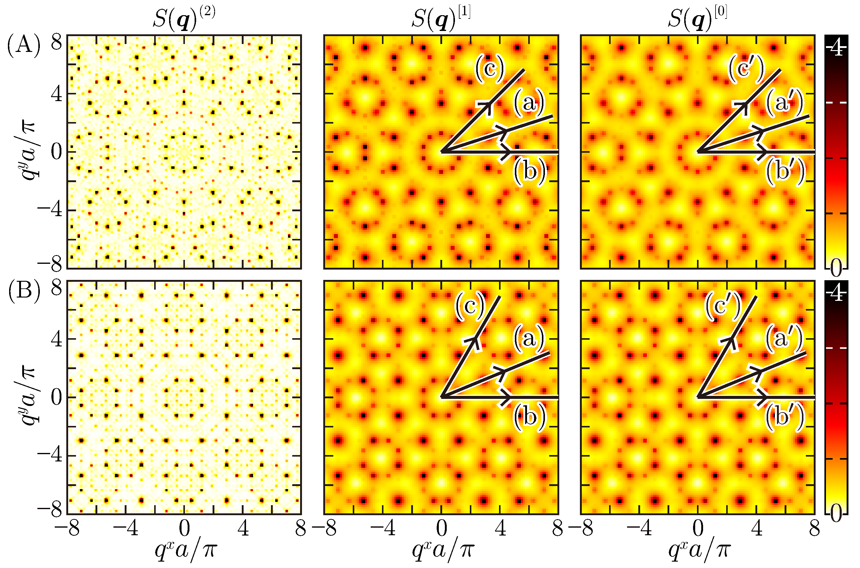
4.1. Static Structure Factors

Before investigating the dynamic structure factors as functions of momentum and energy, we probe the static structure factors to reveal momenta corresponding to magnetic Bragg peaks. We present those for the Penrose and Ammann–Beenker lattices in Figure 4A,B, respectively. Demanding that the quantities (29) and (28) be real immediately yields that $S^{\lambda \lambda }{(-\mathit{q})}^{\left[m\right]}=S^{\lambda \lambda }{\left(\mathit{q}\right)}^{\left[m\right]}$ and $S^{\lambda \lambda }{(-\mathit{q})}^{\left(2\right)}=S^{\lambda \lambda }{\left(\mathit{q}\right)}^{\left(2\right)}$. An n-fold rotational symmetry of the background lattice ensures the same symmetry in the momentum space, $S^{\lambda \lambda }{\left(C_n\mathit{q}\right)}^{\left[m\right]}=S^{\lambda \lambda }{\left(\mathit{q}\right)}^{\left[m\right]}$ and $S^{\lambda \lambda }{\left(C_n\mathit{q}\right)}^{\left(2\right)}=S^{\lambda \lambda }{\left(\mathit{q}\right)}^{\left(2\right)}$. Therefore, an n-fold-rotation-invariant lattice yields a reciprocal lattice of ${\mathbf{C}}_{n\mathrm{h}}$ point symmetry. In two dimensions, ${\mathbf{C}}_{n\mathrm{h}}$ is isomorphic to ${\mathbf{C}}_{2n}$ (${\mathbf{C}}_n$) when n is odd (even). We are thus convinced of the ten- and eight-fold-rotation-invariant $S{\left(\mathit{q}\right)}^{\left(2\right)}\equiv {\sum }_{\lambda =x,y,z}{S}^{\lambda \lambda }{\left(\mathit{q}\right)}^{\left(2\right)}$ and $S{\left(\mathit{q}\right)}^{\left[m\right]}\equiv {\sum }_{\lambda =x,y,z}{S}^{\lambda \lambda }{\left(\mathit{q}\right)}^{\left[m\right]}$ for the Penrose (Figure 4A) and Ammann–Beenker (Figure 4B) lattices, respectively.

Quantum fluctuations dull all the magnetic Bragg peaks more or less, but their positions remain unchanged, evidencing that a collinear long-range order of the ${180}^{\circ }$ Néel type is robust on both Penrose and Ammann–Beenker lattices. While the classical static structure factor $S{\left(\mathit{q}\right)}^{\left(2\right)}$ is made only of longitudinal spin correlations, the quantum corrections $S{\left(\mathit{q}\right)}^{\left[m\right]}$ are relevant to both transverse and longitudinal components. Both corrections are similarly effective on the momenta corresponding to the magnetic Bragg peaks though the transverse components are dominant.

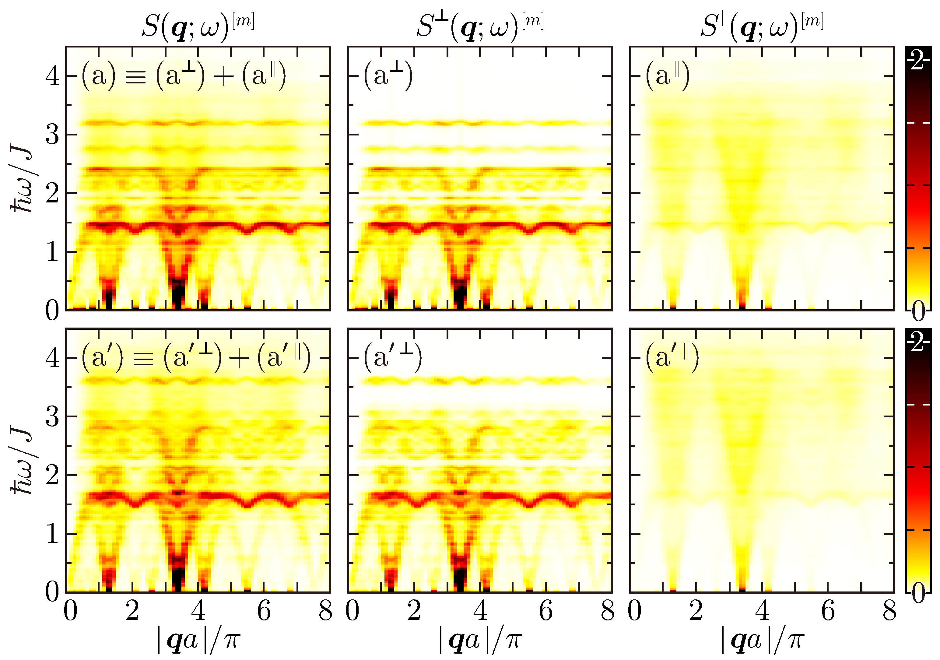
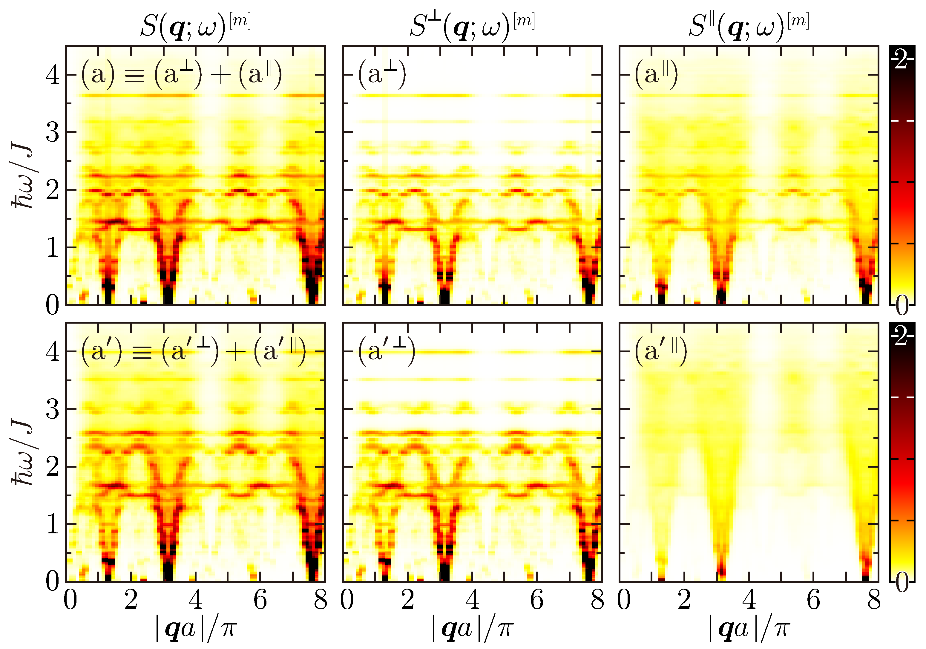
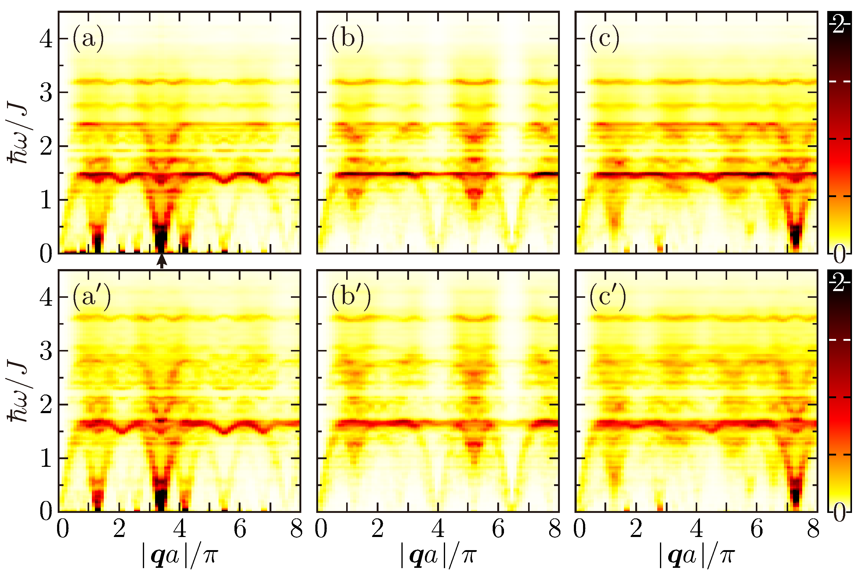
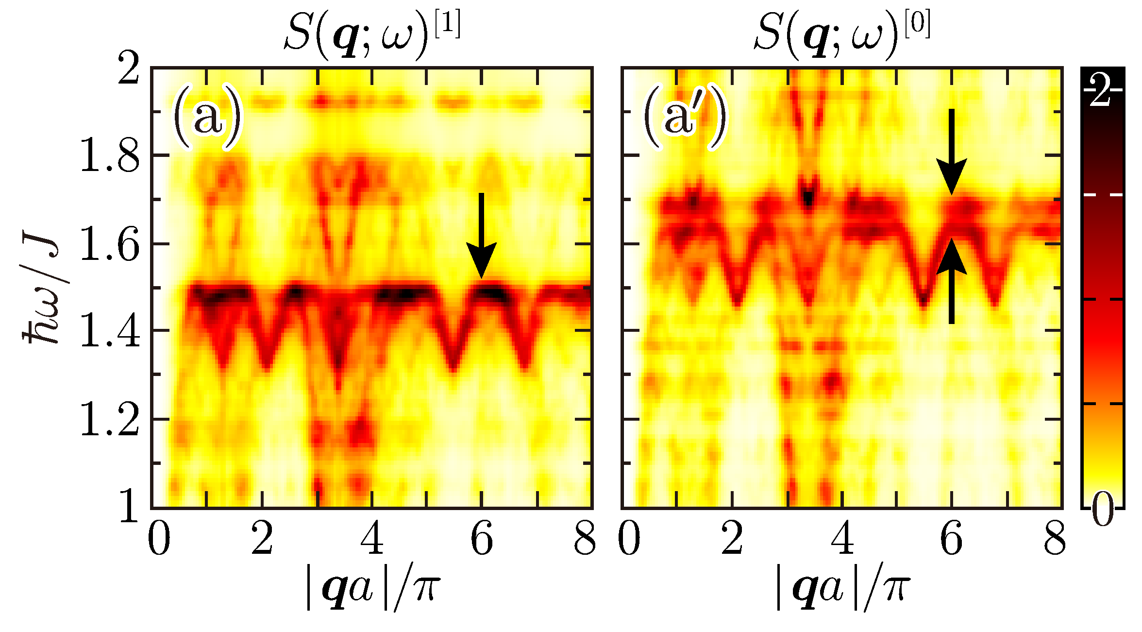
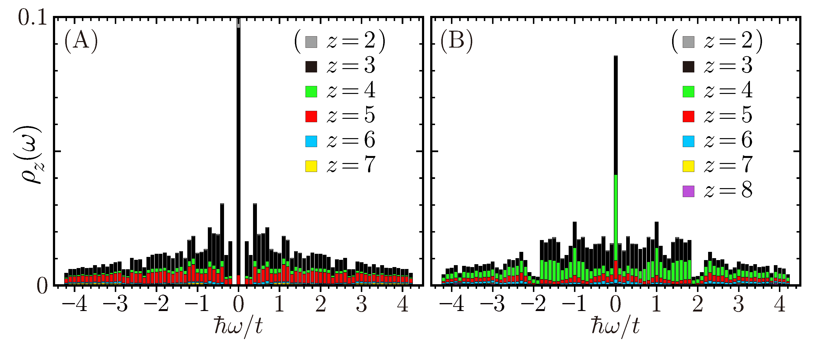
4.2. Dynamic Structure Factors

Figure 5 and Figure 6 show SW calculations of the dynamic structure factors $S{(\mathit{q};\omega )}^{\left[m\right]}\equiv S^{\perp }{(\mathit{q};\omega )}^{\left[m\right]}$ $+S^{\Vert }{(\mathit{q};\omega )}^{\left[m\right]}$ for the $S={\displaystyle \frac{1}{2}}$ Heisenberg antiferromagnets (3) on the Penrose and Ammann–Beenker lattices, respectively, within and beyond the harmonic-oscillator approximation. The transverse component $S^{\perp }{(\mathit{q};\omega )}^{\left[m\right]}$ predominates the longitudinal component $S^{\Vert }{(\mathit{q};\omega )}^{\left[m\right]}$ in spectral weight, especially for the Penrose lattice, when compared to the Ammann–Beenker lattice, and relatively at $m=0$, when compared to $m=1$ (See Appendix A). For both lattices, a linear soft mode appears at every magnetic Bragg wavevector and nearly or fairly flat bands, signifying magnetic excitations localized in some way, lie at several different energies in a self-similar manner. There is a possibility of a gapless mode and a flat mode coexisting in periodic systems as well as in the case with ordered kagome-lattice antiferromagnets [50,51,52]. Schwinger bosons [50] and Holstein–Primakoff bosons [51,52] applied to nearest-neighbor Heisenberg antiferromagnets on the regular kagome lattice both yield a Nambu–Goldstone mode of the long-range Néel order, whether of the $\sqrt{3}\times \sqrt{3}$ or $\mathit{Q}=\mathbf{0}$ type, and a dispersionless branch consisting of excitations localized to an arbitrary hexagon of nearest-neighbor spins [53]. The wholly flat band is gapless or gapfull according as whether or not SWs are brought into interaction and/or modification [52]. However, there is no self-similar structure in these findings.

When we compare the scattering bands of dispersionless character for the Penrose and Ammann–Beenker lattices, both lying around $\hslash \omega =1.5J$ in the LSW formalism and shifting upward in the ISW formalism, those for the Penrose lattice are much flatter in every direction and much stronger in spectral weight. In order to reveal to what types of magnetic excitations the Penrose lattice owe its nearly flat band and the Ammann–Beenker lattice owe its similar but different bandlike segments of modulated spectral weight, we plot in Figure 7 the site-resolved density of states

$$\begin{array}{cc}\hfill & \rho {\left(\omega \right)}^{\left[m\right]}=\sum _{l=1}^L{\rho }_l{\left(\omega \right)}^{\left[m\right]}=\sum _{z=z_{\min }}^{z_{\max }}{\rho }_z{\left(\omega \right)}^{\left[m\right]}\hfill \\ \hfill & =\sum _{z=z_{\min }}^{z_{\max }}{\displaystyle \frac{1}{L}}\left\{\sum _{k_{-}=1}^{L_{-}}{\displaystyle \frac{{\sum }_{i(z_i=z)}{\left|s_{i,k_{-}}^{\left[m\right]}\right|}^2+{\sum }_{j(z_j=z)}{\left|v_{j,k_{-}}^{\left[m\right]}\right|}^2}{{\sum }_{i\in \mathrm{A}}{\left|s_{i,k_{-}}^{\left[m\right]}\right|}^2+{\sum }_{j\in \mathrm{B}}{\left|v_{j,k_{-}}^{\left[m\right]}\right|}^2}}\delta \left(\hslash \omega -{\epsilon }_{k_{-}}^{-\left[m\right]}\right)\right.\hfill \\ \hfill & \left.+\sum _{k_{+}=1}^{L_{+}}{\displaystyle \frac{{\sum }_{i(z_i=z)}{\left|u_{i,k_{+}}^{\left[m\right]}\right|}^2+{\sum }_{j(z_j=z)}{\left|t_{j,k_{+}}^{\left[m\right]}\right|}^2}{{\sum }_{i\in \mathrm{A}}{\left|u_{i,k_{+}}^{\left[m\right]}\right|}^2+{\sum }_{j\in \mathrm{B}}{\left|t_{j,k_{+}}^{\left[m\right]}\right|}^2}}\delta \left(\hslash \omega -{\epsilon }_{k_{+}}^{+\left[m\right]}\right)\right\}\hfill \end{array}$$

(30)

of their LSW ($m=1$) and ISW ($m=0$) excitation spectra. For the Ising antiferromagnet, any spin deviation is immobile and its SW excitation spectrum exactly consists of $z_{\max }-z_{\min }+1$ discrete eigenlevels of energy $zSJ$. With this in mind, we take a keen interest in the highly degenerate LSW eigenstates of energy $\hslash \omega =1.5J$ for the Heisenberg antiferromagnet on the Penrose lattice (Figure 7A), which are essentially composed of tricoordinated sites only and therefore whose energy can be interpreted as $zSJ={\displaystyle \frac{3}{2}}J$. Hence, it follows that they are no different from immobile antiferromagnons emergent on tricoordinated sites in the Ising limit. Then, the lowest-lying nearly flat scattering band of $\hslash \omega =1.5J$ detected in Figure 5a–c reads as an evidence of antiferromagnons strongly confined within sites of $z=3$. For the Heisenberg antiferromagnet on the Ammann–Beenker lattice, on the other hand, much less states concentrate on a particular energy. Indeed, there are still LSW eigenstates of energy $\hslash \omega =1.5J$ existing, but they are here composed of quadricoordinated as well as tricoordinated sites, implying weaker magnon confinement. When LSWs are brought into interaction, the eigenspectrum and therefore scattering spectrum generally shift upward in energy.

The lowest-lying nearly flat scattering band is thus characteristic of the Penrose lattice. It signifies that there exist intriguing antiferromagnons strongly confined within tricoordinated sites. In order to investigate their properties in more detail, we enlarge Figure 5a,a′ around the particular energy $\hslash \omega ={\displaystyle \frac{3}{2}}J$ in Figure 8a,a′. $O\left(S^0\right)$ quantum fluctuations not only push up in energy the nearly flat band but also split it in two, lying at about $1.63J$ and $1.70J$. In Figure 7A′, the ISW eigenstates of $z=3$ character no longer concentrate on a particular energy as the LSW ones, indeed, and their density exhibits a relatively loose peak at around $1.65J$. Such an upward quantum renormalization of the LSW excitation energy is usual with collinear antiferromagnets on bipartite lattices. If we consider the same Hamiltonian as (3) on two-dimensional bipartite periodic lattices such as the quadricoordinated square lattice and tricoordinated honeycomb lattice whose two sublattices are equivalent to each other, $L_{\mathrm{A}}=L_{\mathrm{B}}=L/2\equiv N$, whether L is infinite or finite, its up-to-$O\left(S^0\right)$ bilinear ISW Hamiltonian in the form of (8) is diagonalizable as [44]

$$\begin{array}{cc}\hfill & {\mathcal{H}}_{\mathrm{BL}}^{\left[0\right]}=-NzJ{(S-ϵ)}^2+zJ(S+ϵ)\sum _{\nu =1}^N\sqrt{1-|{\gamma }_{{\mathit{k}}_{\nu }}{|}^2}\sum _{\sigma =\mp }{\alpha }_{{\mathit{k}}_{\nu }}^{\sigma †}{\alpha }_{{\mathit{k}}_{\nu }}^{\sigma };\hfill \\ \hfill & ϵ\equiv {\displaystyle \frac{1}{2}}-{\displaystyle \frac{1}{2N}}\sum _{\nu =1}^N\sqrt{1-|{\gamma }_{{\mathit{k}}_{\nu }}{|}^2},{\gamma }_{{\mathit{k}}_{\nu }}\equiv {\displaystyle \frac{1}{z}}\sum _{\kappa =1}^z{e}^{i{\mathit{k}}_{\nu }·\mathit{\delta }\left(\kappa \right)},\hfill \end{array}$$

(31)

with the set of vectors pointing to z nearest-neighbor sites to ${\mathit{r}}_l$, $\mathit{\delta }\left(1\right)$ to $\mathit{\delta }\left(z\right)$, being no longer dependent on the site index l, where the degenerate ferromagnetic ($\sigma =-$) and antiferromagnetic ($\sigma =+$) quasiparticle magnons are made of the Holstein–Primakoff bosons (4) as

$$\begin{array}{c}\hfill \left\{\begin{array}{c}{\displaystyle {\alpha }_{{\mathit{k}}_{\nu }}^{+}=a_{{\mathit{k}}_{\nu }}^{†}\frac{{\gamma }_{{\mathit{k}}_{\nu }}}{|{\gamma }_{{\mathit{k}}_{\nu }}|}\sinh {\theta }_{{\mathit{k}}_{\nu }}+b_{{\mathit{k}}_{\nu }}\cosh {\theta }_{{\mathit{k}}_{\nu }}}\hfill \\ {\displaystyle {\alpha }_{{\mathit{k}}_{\nu }}^{-}=a_{{\mathit{k}}_{\nu }}\cosh {\theta }_{{\mathit{k}}_{\nu }}+b_{{\mathit{k}}_{\nu }}^{†}\frac{{\gamma }_{{\mathit{k}}_{\nu }}}{|{\gamma }_{{\mathit{k}}_{\nu }}|}\sinh {\theta }_{{\mathit{k}}_{\nu }}}\hfill \end{array}\right.,\left\{\begin{array}{c}{\displaystyle a_{{\mathit{k}}_{\nu }}^{†}=\frac{1}{\sqrt{N}}\sum _{i\in \mathrm{A}}{\mathrm{e}}^{i{\mathit{k}}_{\nu }·{\mathit{r}}_i}{a}_i^{†}}\hfill \\ {\displaystyle b_{{\mathit{k}}_{\nu }}=\frac{1}{\sqrt{N}}\sum _{j\in \mathrm{B}}{\mathrm{e}}^{\mathrm{i}{\mathit{k}}_{\nu }·{\mathit{r}}_j}{b}_j}\hfill \end{array}\right.,\left\{\begin{array}{c}{\displaystyle \cosh 2{\theta }_{{\mathit{k}}_{\nu }}=\frac{1}{\sqrt{1-|{\gamma }_{{\mathit{k}}_{\nu }}{|}^2}}}\hfill \\ {\displaystyle \sinh 2{\theta }_{{\mathit{k}}_{\nu }}=\frac{|{\gamma }_{{\mathit{k}}_{\nu }}|}{\sqrt{1-|{\gamma }_{{\mathit{k}}_{\nu }}{|}^2}}}\hfill \end{array}\right.,\end{array}$$

(32)

whether within or beyond the harmonic-oscillator approximation. Interestingly, besides sharing the Bogoliubov transformation, the LSWs and up-to-$O\left(S^0\right)$ ISWs have similar energies ${\epsilon }_{{\mathit{k}}_{\nu }}^{\left[1\right]}=zS\sqrt{1-|{\gamma }_{{\mathit{k}}_{\nu }}{|}^2}J$ and ${\epsilon }_{{\mathit{k}}_{\nu }}^{\left[0\right]}=z(S+ϵ)\sqrt{1-|{\gamma }_{{\mathit{k}}_{\nu }}{|}^2}J$ [45,54], respectively, which are obtainable from each other via a wavevector-independent renormalization. For the periodic square-lattice antiferromagnet, for instance, the set of wavevectors as good quantum numbers, ${\mathit{k}}_1$ to ${\mathit{k}}_N$, can be expressed as

$$\begin{array}{c}\hfill {\mathit{k}}_{\nu }\equiv {\mathit{k}}_{({\nu }^{\left(1\right)},{\nu }^{\left(2\right)})}=\sum _{n=1}^2\left({\displaystyle \frac{{\nu }^{\left(n\right)}}{\sqrt{N}}}-{\displaystyle \frac{1}{2}}\right)\tilde{\mathit{g}}\left(n\right);\nu =\sum _{n=1}^2\left({\nu }^{\left(n\right)}-1\right){\left(\sqrt{N}\right)}^{n-1}+1,{\nu }^{\left(n\right)}=1,2,\cdots ,\sqrt{N}\end{array}$$

(33)

in terms of the primitive translation vectors in the reciprocal space corresponding to each sublattice A or B,

$$\begin{array}{c}\hfill \tilde{\mathit{g}}\left(1\right)={\displaystyle \frac{\pi }{a}}{\displaystyle \frac{\tilde{\mathit{\delta }}\left(1\right)}{a}},\tilde{\mathit{g}}\left(2\right)={\displaystyle \frac{\pi }{a}}{\displaystyle \frac{\tilde{\mathit{\delta }}\left(2\right)}{a}};\tilde{\mathit{\delta }}\left(1\right)\equiv \mathit{\delta }\left(1\right)+\mathit{\delta }\left(2\right),\tilde{\mathit{\delta }}\left(2\right)\equiv \mathit{\delta }\left(1\right)-\mathit{\delta }\left(2\right);\tilde{\mathit{\delta }}\left(n\right)·\tilde{\mathit{g}}\left(n^{\prime }\right)=2\pi {\delta }_{n{n}^{\prime }},\end{array}$$

(34)

and its up-to-$O\left(S^0\right)$ antiferromagnons exhibit no dispersion on the magnetic Brillouin zone boundary, i.e., along the line connecting ${\displaystyle \frac{\pi }{a}}(1,0)$ and ${\displaystyle \frac{\pi }{a}}({\displaystyle \frac{1}{2}},{\displaystyle \frac{1}{2}})$. In the case of $S={\displaystyle \frac{1}{2}}$, the $O\left(S^0\right)$ quantum renormalization factor ${\epsilon }_{{\mathit{k}}_{\nu }}^{\left[0\right]}/{\epsilon }_{{\mathit{k}}_{\nu }}^{\left[1\right]}$ reads $1.157947$. The up-to-$O\left(S^0\right)$ modified SW theory [45] and equivalent Auerbach–Arovas’ Schwinger–boson mean-field theory [55] consequently derive such quantum renormalization of SW ridges in the dynamic structure factor. If we discuss the SW dynamics in the Penrose-lattice Heisenberg antiferromagnet by analogy, its $O\left(S^0\right)$ quantum renormalization factor ${\epsilon }_{{\mathit{k}}_{\nu }}^{\left[0\right]}/{\epsilon }_{{\mathit{k}}_{\nu }}^{\left[1\right]}$ is indeed larger than unity but looks blurry, extending between $1.63/1.5\simeq 1.09$ and $1.70/1.5\simeq 1.13$. In order to find out why such a split is generated in the lowest-lying nearly flat scattering band and clarify whether or not the split two are still confined within tricoordinated sites, we move to the perpendicular space.

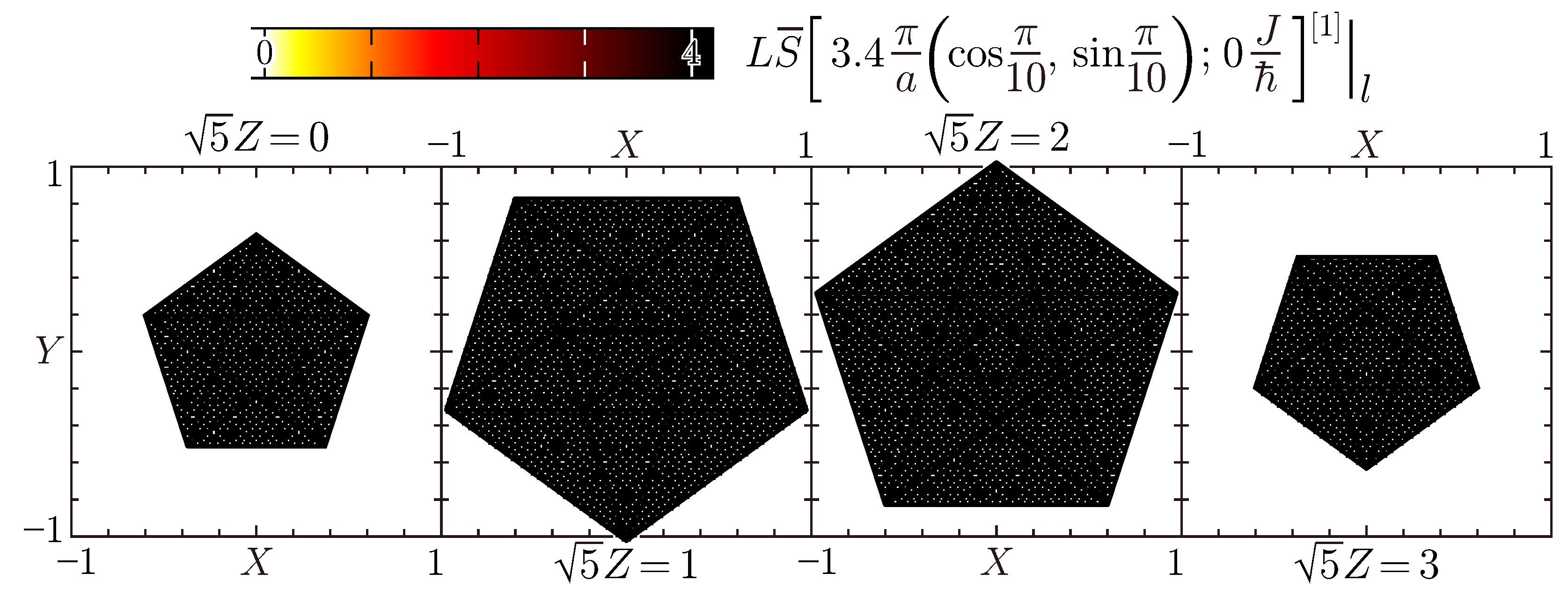
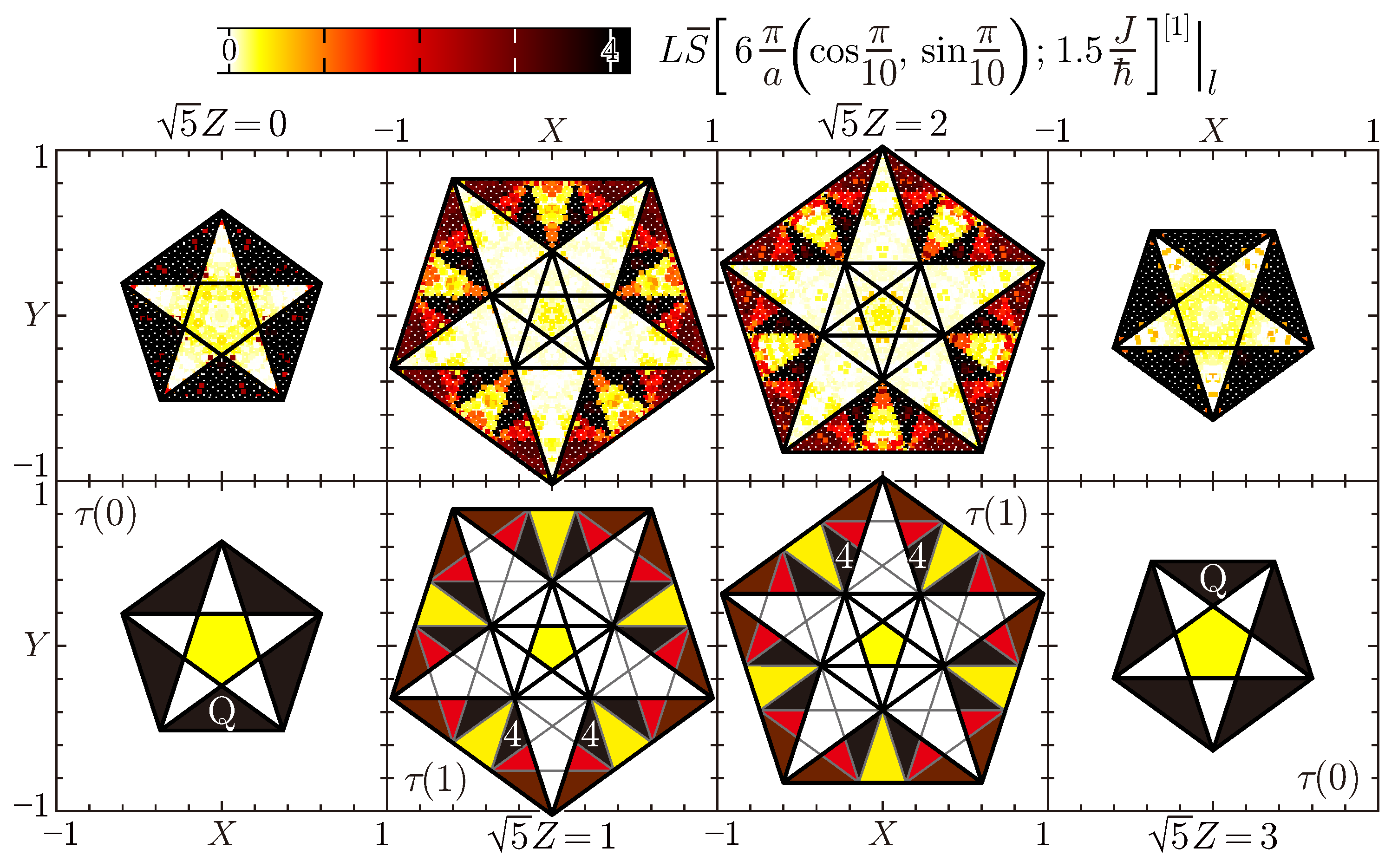
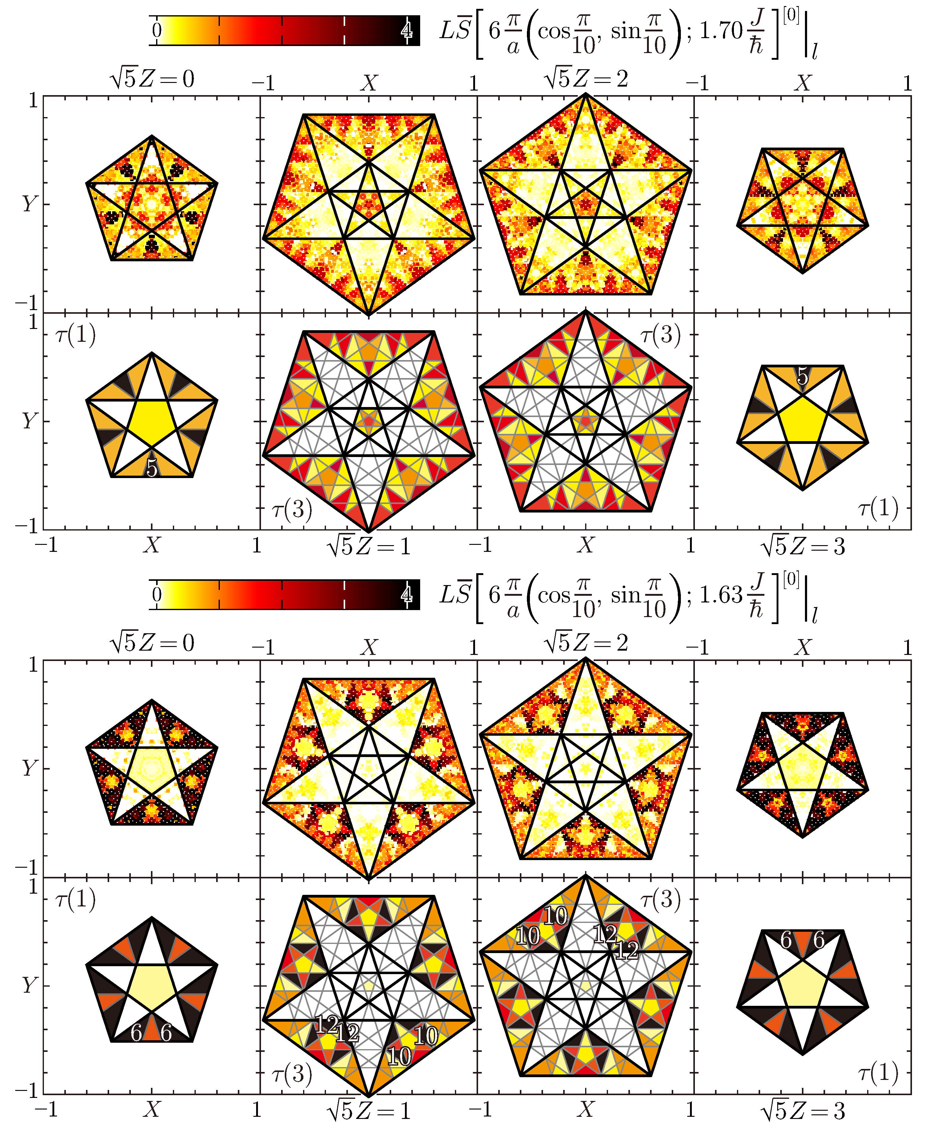
4.3. Perpendicular-Space Analysis

Suppose we define the site-resolved dynamic structure factors

$$\begin{array}{cc}\hfill & S^{\lambda \lambda }{(\mathit{q};\omega )}^{\left[m\right]}\equiv \sum _{l=1}^L{S}^{\lambda \lambda }{(\mathit{q};\omega )}^{\left[m\right]}{|}_l=\sum _{l,l^{\prime }=1}^L{\displaystyle \frac{e^{i\mathit{q}·({\mathit{r}}_l-{\mathit{r}}_{l^{\prime }})}}{2\pi \hslash L}}{\int }_{-\infty }^{\infty }{\hspace{0.25em}}^{\left[m\right]}\langle 0|\delta S_{{\mathit{r}}_l}^{\lambda }\left(t\right)\delta S_{{\mathit{r}}_{l^{\prime }}}^{\lambda }{|0\rangle }^{\left[m\right]}{e}^{i\omega t}dt.\hfill \end{array}$$

(35)

They can be expressed in terms of the coefficients explicitly given in (25) as

$$\begin{array}{cc}\hfill & S^{\perp }{(\mathit{q};\omega )}^{\left[m\right]}{|}_l\equiv S^{xx}{(\mathit{q};\omega )}^{\left[m\right]}{|}_l+S^{yy}{(\mathit{q};\omega )}^{\left[m\right]}{|}_l={\displaystyle \frac{1}{2}}\sum _{\sigma =\mp }\sum _{k_{\sigma }=1}^{L_{\sigma }}\left[{\tilde{\Lambda }}_{\sigma }^{\left({\displaystyle \frac{1}{2}}\right)}(l,\mathit{q};k_{\sigma }){\Lambda }_{\sigma }^{\left({\displaystyle \frac{1}{2}}\right)}{(\mathit{q};k_{\sigma })}^{\ast }\right.\hfill \end{array}$$

$$\begin{array}{cc}\hfill & +\left.{\tilde{\Lambda }}_{\sigma }^{\left({\displaystyle \frac{1}{2}}\right)}(l,\mathit{q};k_{\sigma }){\Lambda }_{\sigma }^{(-{\displaystyle \frac{1}{2}})}{(\mathit{q};k_{\sigma })}^{\ast }+{\Lambda }_{\sigma }^{\left({\displaystyle \frac{1}{2}}\right)}(\mathit{q};k_{\sigma }){\tilde{\Lambda }}_{\sigma }^{(-{\displaystyle \frac{1}{2}})}{(l,\mathit{q};k_{\sigma })}^{\ast }\right]\delta \left(\hslash \omega -{\epsilon }_{k_{\sigma }}^{\sigma \left[m\right]}\right),\hfill \end{array}$$

(36)

$$\begin{array}{cc}\hfill & S^{\Vert }{(\mathit{q};\omega )}^{\left[m\right]}{|}_l\equiv S^{zz}{(\mathit{q};\omega )}^{\left[m\right]}{|}_l=\sum _{k_{-}=1}^{L_{-}}\sum _{k_{+}=1}^{L_{+}}\left[{\tilde{N}}_{-+}^{\left(0\right)}(l,\mathit{q};k_{-},k_{+})N_{-+}^{\left(0\right)}{(\mathit{q};k_{-},k_{+})}^{\ast }\right]\delta \left(\hslash \omega -{\epsilon }_{k_{-}}^{-\left[m\right]}-{\epsilon }_{k_{+}}^{+\left[m\right]}\right),\hfill \end{array}$$

(37)

where ${\tilde{\Lambda }}_{\sigma }^{(\pm {\displaystyle \frac{1}{2}})}$ read ${\tilde{D}}_{-}^{(\pm {\displaystyle \frac{1}{2}})}$ ($\sigma =-$) or ${\tilde{C}}_{+}^{(\pm {\displaystyle \frac{1}{2}})}$ ($\sigma =+$) just like ${\Lambda }_{\sigma }^{(\pm {\displaystyle \frac{1}{2}})}$ in (26). In order to recover the point symmetry $\mathbf{P}$ of the original dynamic structure factor $S{(\mathit{q};\omega )}^{\left[m\right]}\equiv {\sum }_{\lambda =x,y,z}{S}^{\lambda \lambda }{(\mathit{q};\omega )}^{\left[m\right]}$ and thereby extract site-resolved spectral weights of real definite from it, we resymmetrize the site-resolved dynamic structure factors $S{(\mathit{q};\omega )}^{\left[m\right]}{|}_l\equiv {\sum }_{\lambda =x,y,z}{S}^{\lambda \lambda }{(\mathit{q};\omega )}^{\left[m\right]}{|}_l$ into

$$\begin{array}{c}\hfill \overline{S}{(\mathit{q};\omega )}^{\left[m\right]}{|}_l\equiv {\displaystyle \frac{1}{g^{\mathbf{P}}}}\sum _{p\in \mathbf{P}}S{(p\mathit{q};\omega )}^{\left[m\right]}{|}_l,\end{array}$$

(38)

where $g^{\mathbf{P}}$ is the order of $\mathbf{P}$. The Penrose lattice demands that $\mathbf{P}={\mathbf{C}}_{5\mathrm{h}}$.

In the context of making a perpendicular-space analysis of the flat bands signifying confined states, it is worth observing linear soft modes similarly. Figure 9 is a perpendicular-space mapping of $L\overline{S}{(\mathit{q};\omega )}^{\left[1\right]}{|}_l$ at momenta corresponding to the strongest magnetic Bragg spots. The spectral weighting is uniform and over the entire perpendicular space, evidencing that soft modes at low energies involve all sites of $z=3$ to 7. The plot of $L\overline{S}{(\mathit{q};\omega )}^{\left[0\right]}{|}_l$ at the same momenta and zero energy remains almost the same.

With the above in mind, let us observe the lowest-lying nearly flat scattering band peculiar to the Penrose lattice in its perpendicular space. Figure 10 is a perpendicular-space mapping of $L\overline{S}{(\mathit{q};\omega )}^{\left[1\right]}{|}_l$ at the wavevector $(q^x,q^y)=6{\displaystyle \frac{\pi }{a}}(cos{\displaystyle \frac{\pi }{10}},sin{\displaystyle \frac{\pi }{10}})$ and energy $\hslash \omega =1.5J$ on the nearly flat LSW-scattering band (Figure 8a). Now, the spectral weighting is far from uniform and localizes on the D and Q domains in the perpendicular space labeled by the $\tau \left(0\right)$ indices, evidencing that the LSW nearly flat mode at around the particular energy ${\displaystyle \frac{3}{2}}J$ belongs to tricoordinated sites. A careful observation leads us to find out that the D domains are painted with several different colors compatibly with sublabels $\tau \left(1\right)$ as well. In terms of the $\tau \left(1\right)$ language, the spectral weights of the lowest-lying nearly flat LSW scattering band center on the subdomains 4, 5, and 6, the former one of which resides in the $\tau \left(0\right)=\mathrm{D}$ domain, while the rest of which reside in the $\tau \left(0\right)=\mathrm{Q}$ domain, and much less ooze out to the subdomains 1 to 3, all residing in the $\tau \left(0\right)=\mathrm{D}$ domain. If we sum up the coordination numbers of nearest-neighbor ($R=1$) sites at ${\mathit{r}}_{l^{\prime }}$ to its core ($R=0$) site at ${\mathit{r}}_l$, the three subdomains 4 to 6 in the $\tau \left(1\right)$ language can be classified into two groups, $\left\{5\right\}$ with ${\sum }_{l^{\prime }}{z}_{l^{\prime }}\left(1\right)=16$ and $\{4,6\}$ with ${\sum }_{l^{\prime }}{z}_{l^{\prime }}\left(1\right)=17$ (See

Table 1. The way of numbering local environments of $R=1$ for the Penrose lattice. All the vertices are classified into 15 subtypes and labeled $\tau \left(1\right)=1$ to 15, according to how many vertices of the types D to S3 appear at distances $R=0$ and 1, when we truncate their surrounding vertices at a distance of $R=1$. In an attempt to characterize each environment, we sum up the coordination numbers of nearest-neighbor ($R=1$) sites at ${\mathit{r}}_{l^{\prime }}$ to its core ($R=0$) site at ${\mathit{r}}_l$.

$\mathit{\tau }\left(1\right)$	D ($\mathit{z}=3$)	Q ($\mathit{z}=3$)	K ($\mathit{z}=4$)	J ($\mathit{z}=5$)	S ($\mathit{z}=5$)	S5 ($\mathit{z}=5$)	S4 ($\mathit{z}=6$)	S3 ($\mathit{z}=7$)	${\sum }_{{\mathit{l}}^{\prime }}{\mathit{z}}_{{\mathit{l}}^{\prime }} \left(1\right)$
1	(1;0)	(0;0)	(0;1)	(0;1)	(0;0)	(0;0)	(0;1)	(0;0)	15
2	(1;0)	(0;0)	(0;1)	(0;1)	(0;0)	(0;0)	(0;0)	(0;1)	16
3	(1;0)	(0;0)	(0;0)	(0;2)	(0;1)	(0;0)	(0;0)	(0;0)	15
4	(1;0)	(0;0)	(0;0)	(0;1)	(0;1)	(0;0)	(0;0)	(0;1)	17
5	(0;0)	(1;0)	(0;0)	(0;2)	(0;0)	(0;0)	(0;1)	(0;0)	16
6	(0;0)	(1;0)	(0;0)	(0;2)	(0;0)	(0;0)	(0;0)	(0;1)	17
7	(0;2)	(0;0)	(1;0)	(0;2)	(0;0)	(0;0)	(0;0)	(0;0)	16
8	(0;2)	(0;2)	(0;0)	(1;0)	(0;0)	(0;1)	(0;0)	(0;0)	17
9	(0;2)	(0;2)	(0;0)	(1;0)	(0;0)	(0;0)	(0;1)	(0;0)	18
10	(0;2)	(0;1)	(0;1)	(1;0)	(0;0)	(0;0)	(0;1)	(0;0)	19
11	(0;2)	(0;0)	(0;2)	(1;0)	(0;0)	(0;0)	(0;0)	(0;1)	21
12	(0;5)	(0;0)	(0;0)	(0;0)	(1;0)	(0;0)	(0;0)	(0;0)	15
13	(0;0)	(0;0)	(0;0)	(0;5)	(0;0)	(1;0)	(0;0)	(0;0)	25
14	(0;2)	(0;1)	(0;0)	(0;3)	(0;0)	(0;0)	(1;0)	(0;0)	24
15	(0;4)	(0;2)	(0;0)	(0;1)	(0;0)	(0;0)	(0;0)	(1;0)	23

again). This categorization plays a key role in understanding the split in the nearly flat scattering band on the occurrence of interaction between LSWs.

Figure 11 presents perpendicular-space mappings of $L\overline{S}{(\mathit{q};\omega )}^{\left[0\right]}{|}_l$ at the same wavevector as Figure 10 and energies $\hslash \omega =1.70J$ and $\hslash \omega =1.63J$ on the interaction-driven higher- and lower-lying split branches (Figure 8a′) of the otherwise degenerate single nearly flat scattering band. Both spectral weightings still localize on the D and/or Q domains, evidencing that scattering magnons that form these two separate nearly flat bands are still well confined within tricoordinated sites, more intriguingly claiming that they each are “superconfined” within selected tricoordinated sites. The ISW ways of painting the D and Q domains are more complicated such that the Q domains are divided into $\tau \left(1\right)$ subdomains, while the $\tau \left(1\right)=4$ subdomains in the D domains are further partitioned into numerous $\tau \left(3\right)$ subdomains. So far as the two ISW nearly flat modes are concerned, tricoordinated $\tau \left(0\right)=\mathrm{Q}$ sites split into two types of subgroups $\tau \left(1\right)=5$ and $\tau \left(1\right)=6$, whereas tricoordinated $\tau \left(1\right)=4$ sites split into three types of subgroups $\tau \left(3\right)=10$ to 12. The spectral weights of the higher-lying nearly flat ISW scattering band center roughly on the subdomain $\tau \left(1\right)=5$ with ${\sum }_{l^{\prime }}{z}_{l^{\prime }}\left(1\right)=16$, while those of the lower-lying one center chiefly on the subdomains $\tau \left(1\right)=6$, $\tau \left(3\right)=10$, and $\tau \left(3\right)=12$ all with ${\sum }_{l^{\prime }}{z}_{l^{\prime }}\left(1\right)=17$. The $O\left(S^0\right)$ interactions prefer the higher-coordinated local environments labeled $\tau \left(1\right)=4$ and $\tau \left(1\right)=6$ to the lower-coordinated ones labeled $\tau \left(1\right)=5$, and they further choose the relatively high-coordinated local environments labeled $\tau \left(3\right)=10$ and $\tau \left(3\right)=12$ among the $\tau \left(1\right)=4$ subdomains, splitting the otherwise degenerate single nearly flat scattering band into two bands. The lower (higher)-lying one is mediated by $O\left(S^0\right)$-interaction-stabilized (destabilized) magnons “superconfined” within particular tricoordinated sites surrounded by a larger (smaller) number of bonds. Confined antiferromagnons of $z=3$ character are robust against quantum fluctuations and the $1/S$ corrections put them into “superconfinement”.

5. Summary and Discussion

Since the half-filled single-band Hubbard model reduces to our spin-${\displaystyle \frac{1}{2}}$ antiferromagnetic Heisenberg model in question in its strong-correlation limit, it is worthwhile to compare the above-revealed confined antiferromagnons with their fermionic origins. A pioneering calculation [10] was carried out for the vertex-model tight-binding Hamiltonian

$$\begin{array}{cc}\hfill & {\mathcal{H}}_t=-t\sum _{\sigma =\uparrow ,\downarrow }\sum _{i\in \mathrm{A}}\sum _{j\in \mathrm{B}}{l}_{i,j}(c_{i:\sigma }^{†}{c}_{j:\sigma }+c_{j:\sigma }^{†}{c}_{i:\sigma })=\sum _{\sigma =\uparrow ,\downarrow }{\mathbf{c}}_{\sigma }^{†}\mathbf{M}{\mathbf{c}}_{\sigma };\hfill \\ \hfill & {\mathit{c}}_{\sigma }^{†}=\left[c_{1:\sigma }^{†},\cdots ,c_{L_{\mathrm{A}}:\sigma }^{†},c_{L_{\mathrm{A}}+1:\sigma }^{†},\cdots ,c_{L_{\mathrm{A}}+L_{\mathrm{B}}:\sigma }^{†}\right],\hfill \\ \hfill & \mathbf{M}=\left[\begin{array}{ccc}{\mathbf{O}}_{L_{\mathrm{A}}}& |& \mathbf{C}\\ {\mathbf{C}}^{†}& |& {\mathbf{O}}_{L_{\mathrm{B}}}\end{array}\right],{\left[{\mathbf{O}}_{L_{\mathrm{A}}}\right]}_{i,i^{\prime }}={\left[{\mathbf{O}}_{L_{\mathrm{B}}}\right]}_{j,j^{\prime }}=0,{\left[\mathbf{C}\right]}_{i,j}=-t{l}_{i,j},\hfill \end{array}$$

(39)

on the two-dimensional Penrose lattice, where $c_{l:\sigma }^{†}$ creates an electron with spin $\sigma$ at site ${\mathit{r}}_l$ positioned on vertices of rhombuses, ${\mathit{c}}_{\sigma }^{†}$ is a row vector of dimension L, ${\mathbf{O}}_{L_{\mathrm{A}}}$ and ${\mathbf{O}}_{L_{\mathrm{B}}}$ are zero matrices of dimension $L_{\mathrm{A}}\times L_{\mathrm{A}}$ and $L_{\mathrm{B}}\times L_{\mathrm{B}}$, respectively. An ordinary unitary transformation

$$\begin{array}{c}\hfill {\mathit{c}}_{\sigma }=\mathbf{U}{\mathit{\alpha }}_{\sigma };{\left[\mathbf{U}\right]}_{l,k}\equiv u_{l,k},{\mathit{\alpha }}_{\sigma }^{†}\equiv \left[{\alpha }_{1:\sigma }^{†},\cdots ,{\alpha }_{L:\sigma }^{†}\right]\end{array}$$

(40)

rewriting (39) gives

$$\begin{array}{c}\hfill {\mathcal{H}}_t=\sum _{\sigma =\uparrow ,\downarrow }\sum _{k=1}^L{\epsilon }_k{\alpha }_{k:\sigma }^{†}{\alpha }_{k:\sigma },\end{array}$$

(41)

where ${\alpha }_{k:\sigma }^{†}$ creates a quasiparticle fermion with spin $\sigma$ of energy ${\epsilon }_k$. While ${\epsilon }_k$ is no longer a cosine band on any quasiperiodic lattice, this Hamiltonian at half filling possesses the electron-hole symmetry—electrons with energy above the Fermi sea behave the same as holes emergent in the Fermi sea. It is nowadays well known that the Hamiltonian ${\mathcal{H}}_t$ yields macroscopically degenerate confined states of ${\epsilon }_k=0$ on not only the Penrose [10,11,20] but also Ammann–Beenker [41,56] lattices. In order to see which sites form these confined states, we plot in Figure 12 the site-resolved density of states

$$\begin{array}{c}\hfill \rho \left(\omega \right)=\sum _{l=1}^L{\rho }_l\left(\omega \right)=\sum _{z=z_{\min }}^{z_{\max }}{\rho }_z\left(\omega \right)=\sum _{z=z_{\min }}^{z_{\max }}{\displaystyle \frac{1}{L}}\sum _{k=1}^L{\displaystyle \frac{{\sum }_{l(z_l=z)}{|u_{l,k}|}^2}{{\sum }_{l=1}^L{|u_{l,k}|}^2}}\delta \left(\hslash \omega -{\epsilon }_k\right)\end{array}$$

(42)

of the quasiparticle fermion excitation spectrum. For the Penrose lattice, the $\delta$-function peak at $\hslash \omega =0$ accounts for about 10 percent of the total number of states, which consists of strictly localized states—confined within sites of $z=3$ and $z=5$—separated from the remainder of the states—two symmetric continuum—by a gap $0.172871t$ [11,20]. We find a macroscopically degenerate $\delta$-function-like peak at $\hslash \omega =0$ for the Ammann–Beenker lattice as well. While its constituent states involve all types of sites, they are each still confined [41]. All of these similarities and differences between the Penrose and Ammann–Beenker lattices are shown in Figure 7.

We can see at a glance the spatial confinement of the zero-energy degenerate states of the tight-binding Hamiltonian (39) on the Penrose lattice in Figure 13a. All the confined states are separated from each other by “forbidden ladders” [11,20]—one-dimensional unbranched closed loops with no wavefunction amplitude. Every weighted domain enclosed by forbidden ladders reasonably consists either of tricoordinated sites only or of pentacoordinated plus tricoordinated sites in any case confined in either of the two sublattices. Every forbidden ladder lies between a couple of confined domains made of different sublattices. Without any Coulomb interaction, these confined domains, i.e., tricoordinated and pentacoordinated states, have staggered magnetizations. On-site Coulomb repulsion U emergent to the tight-binding Hamiltonian (39) immediately lifts the degeneracy among its zero-energy states and causes staggered magnetizations on all sites of $z=3$ to 7. The local staggered magnetization on the site at ${\mathit{r}}_l$ as a function of U, $m_l\left(U\right)$, grows linearly with increasing U and dependently on l, $|m_l\left(U\right)-m_l\left(0\right)|\propto {\kappa }_{l}U$ [20], as long as U is sufficiently small, in contrast to the exponential growth free from site dependence with U emergent to a nonmagnetic tight-binding Hamiltonian on any bipartite lattice, $|m_l\left(U\right)|\propto e^{-\kappa /U}$ [57]. Such an unconventional growth of staggered magnetizations can be seen on the Ammann–Beenker [41] and periodic Lieb [58] lattices as well, the latter of which exhibits a flat-band ferromagnetism, $m_l\left(0\right)\ne 0$ only on bicoordinated sites of $z_l=2$. On every quasiperiodic lattice, ${\kappa }_l$ depends on l in a complicated manner because of the lack of translational symmetry, but ${\kappa }_l$ increases as $z_l$ decreases. Tricoordinated sites are magnetized much faster than any other site with increasing U [20,41]. Thus, the confined states made only of tricoordinated sites survive the on-site Coulomb repulsion.

Here, in the strong correlation limit, come the observations in Figure 13b,b′,b″. Longitudinal components in the exchange Hamiltonian (3) bring a local potential on every site. In the LSW Hamiltonian (11), it reads $z_{l}SJ$ [See Equation (11)] to destabilize higher-coordinated sites more. Interestingly enough, Figure 13a with all weighted pentacoordinated sites away coincides with Figure 13b. The alternate arrangement of A- and B-sublattice-confined domains with forbidden ladders in between remains exactly the same between Figure 13a,b. Antiferromagnons are thus confined within only tricoordinated sites. Bringing LSWs into interaction yields more intriguing observations, Figure 13b′,b″, where site potentials are no longer necessarily equal even among sites of the same coordination number because their surrounding environments become effective in the ISW Hamiltonian (12). ISWs yielding the lower- and higher-lying nearly flat scattering bands in Figure 8 look complementary to each other in spatial distribution, whose wavefunction amplitudes, Figure 13b′,b″, add up approximately to the LSW ones, Figure 13b. The lower- and higher-lying nearly flat scattering bands are mediated by antiferromagnons stabilized and destabilized by $O\left(S^0\right)$ interactions, respectively, which are confined within tricoordinated sites surrounded by larger and smaller numbers of bonds, respectively. Quantum fluctuations encourage further confinement of antiferromagnons, which may be referred to as “superconfinement”. Note again that the nearly flat mode in the dynamic structure factor is characteristic of the Penrose lattice and it splits in two due to the variety of its constituent local environments. Superconfined antiferromagnons are thus peculiar to the two-dimensional Penrose lattice.

References

1. Penrose, R. The role of aesthetics in pure and applied mathematical research. Bull. Inst. Math. Appl. 1974, 10, 266. [Google Scholar]
2. Gardner, M. Extraordinary nonperiodic tiling that enriches the theory of tiles. Sci. Am. 1977, 236, 110. [Google Scholar] [CrossRef]
3. Mackay, A.L. Crystallography and the penrose pattern. Physica A 1982, 114, 609. [Google Scholar] [CrossRef]
4. Beenker, F.P.M. Algebraic Theory of Non-Periodic Tilings of the Plane by Two Simple Building Blocks: A Suqare and a Rhombus; T.H.-Report, 82-WSK-04; Eindhoven University of Technology: Eindhoven, The Netherlands, 1982. [Google Scholar]
5. Niizeki, K.; Mitani, H. Two-dimensional dodecagonal quasilattices. J. Phys. A Math. Gen. 1987, 20, L405. [Google Scholar] [CrossRef]
6. Choy, T.C. Density of States for a Two-Dimensional Penrose Lattice: Evidence of a Strong Van Hove Singularity. Phys. Rev. Lett. 1985, 55, 2915. [Google Scholar] [CrossRef] [PubMed]
7. Odagaki, T.; Nguyen, D. Electronic and vibrational spectra of two-dimensional quasicrystals. Phys. Rev. B 1986, 33, 2184. [Google Scholar] [CrossRef] [PubMed]
8. Tsunetsugu, H.; Fujiwara, T.; Ueda, K.; Tokihiro, T. Eigenstates in 2-Dimensional Penrose Tiling. J. Phys. Soc. Jpn. 1986, 55, 1420. [Google Scholar] [CrossRef]
9. Tsunetsugu, H.; Fujiwara, T.; Ueda, K.; Tokihiro, T. Electronic properties of the Penrose lattice. I. Energy spectrum and wave functions. Phys. Rev. B 1991, 43, 8879. [Google Scholar] [CrossRef]
10. Kohmoto, M.; Sutherland, B. Electronic States on a Penrose Lattice. Phys. Rev. Lett. 1986, 56, 2740. [Google Scholar] [CrossRef]
11. Arai, M.; Tokihiro, T.; Fujiwara, T.; Kohmoto, M. Strictly localized states on a two-dimensional Penrose lattice. Phys. Rev. B 1988, 38, 1621. [Google Scholar] [CrossRef]
12. Zijlstra, E.S.; Janssen, T. Density of states and localization of electrons in a tight-binding model on the Penrose tiling. Phys. Rev. B 2000, 61, 3377. [Google Scholar] [CrossRef]
13. de Bruijn, N.G. Algebraic theory of Penrose’s non-periodic tilings of the plane. I. Indag. Math. Proc. Ser. A 1981, 84, 39. Available online: https://www.sciencedirect.com/science/article/pii/1385725881900160 (accessed on 7 July 2024). [CrossRef]
14. de Bruijn, N.G. Algebraic theory of Penrose’s non-periodic tilings of the plane. II. Indag. Math. Proc. Ser. A 1981, 84, 53. Available online: https://www.sciencedirect.com/science/article/pii/1385725881900172 (accessed on 7 July 2024). [CrossRef]
15. Shechtman, D.; Blech, I.; Gratias, D.; Cahn, J.W. Metallic Phase with Long-Range Orientational Order and No Translational Symmetry. Phys. Rev. Lett. 1984, 53, 1951. [Google Scholar] [CrossRef]
16. Tsai, A.P.; Inoue, A.; Masumoto, T. A Stable Quasicrystal in Al-Cu-Fe System. Jpn. J. Appl. Phys. 1987, 26, L1505. [Google Scholar] [CrossRef]
17. Tsai, A.P.; Inoue, A.; Masumoto, T. New Stable Icosahedral Al-Cu-Ru and Al-Cu-Os Alloys. Jpn. J. Appl. Phys. 1988, 27, L1587. [Google Scholar] [CrossRef]
18. Levine, D.; Steinhardt, P.J. Quasicrystals: A New Class of Ordered Structures. Phys. Rev. Lett. 1984, 53, 2477. [Google Scholar] [CrossRef]
19. Levine, D.; Steinhardt, P.J. Quasicrystals. I. Definition and structure. Phys. Rev. B 1986, 34, 596. [Google Scholar] [CrossRef] [PubMed]
20. Koga, A.; Tsunetsugu, H. Antiferromagnetic order in the Hubbard model on the Penrose lattice. Phys. Rev. B 2017, 96, 214402. [Google Scholar] [CrossRef]
21. Sakai, S.; Arita, R.; Ohtsuki, T. Hyperuniform electron distributions controlled by electron interactions in quasicrystals. Phys. Rev. B 2022, 105, 054202. [Google Scholar] [CrossRef]
22. Wessel, S.; Milat, I. Quantum fluctuations and excitations in antiferromagnetic quasicrystals. Phys. Rev. B 2005, 71, 104427. [Google Scholar] [CrossRef]
23. Jagannathan, A.; Szallas, A.; Wessel, S.; Duneau, M. Penrose quantum antiferromagnet. Phys. Rev. B 2007, 75, 212407. [Google Scholar] [CrossRef]
24. Wessel, S.; Jagannathan, A.; Haas, S. Quantum Antiferromagnetism in Quasicrystals. Phys. Rev. Lett. 2003, 90, 177205. [Google Scholar] [CrossRef] [PubMed]
25. Sandvik, A.W. Finite-size scaling of the ground-state parameters of the two-dimensional Heisenberg model. Phys. Rev. B 1997, 56, 11678. [Google Scholar] [CrossRef]
26. Szallas, A.; Jagannathan, A. Spin waves and local magnetizations on the Penrose tiling. Phys. Rev. B 2008, 77, 104427. [Google Scholar] [CrossRef]
27. Inoue, T.; Yamamoto, S. Optical Observation of Quasiperiodic Heisenberg Antiferromagnets in Two Dimensions. Phys. Status Solidi B 2020, 257, 2000118. [Google Scholar] [CrossRef]
28. Inoue, T.; Yamamoto, S. Polarized Raman Response of Two-Dimensional Quasiperiodic Antiferromagnets: Configuration-Interaction versus Green’s Function Approaches. J. Phys. Soc. Jpn. 2022, 91, 053701. [Google Scholar] [CrossRef]
29. Sato, T.J.; Takakura, H.; Tsai, A.P.; Shibata, K.; Ohoyama, K.; Andersen, K.H. Antiferromagnetic spin correlations in the Zn-Mg-Ho icosahedral quasicrystal. Phys. Rev. B 2000, 61, 476. [Google Scholar] [CrossRef]
30. Sato, T.J.; Takakura, H.; Tsai, A.P.; Shibata, K. Magnetic excitations in the Zn-Mg-Tb icosahedral quasicrystal: An inelastic neutron scattering study. Phys. Rev. B 2006, 73, 054417. [Google Scholar] [CrossRef]
31. Sato, T.J.; Kashimoto, S.; Masuda, C.; Onimaru, T.; Nakanowatari, I.; Iida, K.; Morinaga, R.; Ishimasa, T. Neutron scattering study on spin correlations and fluctuations in the transition-metal-based magnetic quasicrystal Zn-Fe-Sc. Phys. Rev. B 2008, 77, 014437. [Google Scholar] [CrossRef]
32. Guidoni, L.; Triché, C.; Verkerk, P.; Grynberg, G. Quasiperiodic Optical Lattices. Phys. Rev. Lett. 1997, 79, 3363. [Google Scholar] [CrossRef]
33. Viebahn, K.; Sbroscia, M.; Carter, E.; Yu, J.-C.; Schneider, U. Matter-Wave Diffraction from a Quasicrystalline Optical Lattice. Phys. Rev. Lett. 2019, 122, 110404. [Google Scholar] [CrossRef] [PubMed]
34. Sbroscia, M.; Viebahn, K.; Carter, E.; Yu, J.-C.; Gaunt, A.; Schneider, U. Observing Localization in a 2D Quasicrystalline Optical Lattice. Phys. Rev. Lett. 2020, 125, 200604. [Google Scholar] [CrossRef] [PubMed]
35. Sanchez-Palencia, L.; Santos, L. Bose-Einstein condensates in optical quasicrystal lattices. Phys. Rev. A 2005, 72, 053607. [Google Scholar] [CrossRef]
36. Jagannathan, A.; Duneau, M. An eightfold optical quasicrystal with cold atoms. Europhys. Lett. 2013, 104, 66003. [Google Scholar] [CrossRef]
37. Jagannathan, A.; Duneau, M. The eight-fold way for optical quasicrystals. Eur. Phys. J. B 2014, 87, 149. [Google Scholar] [CrossRef]
38. Duan, L.-M.; Demler, E.; Lukin, M.D. Controlling Spin Exchange Interactions of Ultracold Atoms in Optical Lattices. Phys. Rev. Lett. 2003, 91, 090402. [Google Scholar] [CrossRef] [PubMed]
39. Lifshitz, R. What is a crystal? Z. Kristallogr. 2007, 222, 313. [Google Scholar] [CrossRef]
40. Ghadimi, R.; Sugimoto, T.; Tohyama, T. Mean-field study of the Bose-Hubbard model in the Penrose lattice. Phys. Rev. B 2020, 102, 224201. [Google Scholar] [CrossRef]
41. Koga, A. Superlattice structure in the antiferromagnetically ordered state in the Hubbard model on the Ammann-Beenker tiling. Phys. Rev. B 2020, 102, 115125. [Google Scholar] [CrossRef]
42. Holstein, T.; Primakoff, H. Field Dependence of the Intrinsic Domain Magnetization of a Ferromagnet. Phys. Rev. 1940, 58, 1098. [Google Scholar] [CrossRef]
43. Yamamoto, S.; Fukui, T.; Maisinger, K.; Schollwöck, U. Combination of ferromagnetic and antiferromagnetic features in Heisenberg ferrimagnets. J. Phys. Condens. Matter 1998, 10, 11033. [Google Scholar] [CrossRef]
44. Noriki, Y.; Yamamoto, S. Modified Spin-Wave Theory on Low-Dimensional Heisenberg Ferrimagnets: A New Robust Formulation. J. Phys. Soc. Jpn. 2017, 86, 034714. [Google Scholar] [CrossRef]
45. Yamamoto, S.; Noriki, Y. Spin-wave thermodynamics of square-lattice antiferromagnets revisited. Phys. Rev. B 2019, 99, 094412. [Google Scholar] [CrossRef]
46. Yamamoto, S. Bosonic representation on one-dimensional Heisenberg ferrimagnets. Phys. Rev. B 2004, 69, 064426. [Google Scholar] [CrossRef]
47. Brehmer, S.; Mikeska, H.-J.; Yamamoto, S. Low-temperature properties of quantum antiferromagnetic chains with alternating spins S=1 and S=1/2. J. Phys. Condens. Matter 1997, 9, 3921. [Google Scholar] [CrossRef]
48. Yamamoto, S.; Fukui, T. Thermodynamic properties of Heisenberg ferrimagnetic spin chains: Ferromagnetic-antiferromagnetic crossover. Phys. Rev. B 1998, 57, R14008(R). [Google Scholar] [CrossRef]
49. Louisell, W.H. Radiation and Noise in Quantum Electronics; McGraw-Hill: New York, NY, USA, 1964; p. 101. [Google Scholar]
50. Messio, L.; Cépas, O.; Lhuillier, C. Schwinger-boson approach to the kagome antiferromagnet with Dzyaloshinskii-Moriya interactions: Phase diagram and dynamical structure factors. Phys. Rev. B 2010, 81, 064428. [Google Scholar] [CrossRef]
51. Chernyshev, A.L.; Zhitomirsky, M.E. Order and excitations in large-S kagome-lattice antiferromagnets. Phys. Rev. B 2015, 92, 144415. [Google Scholar] [CrossRef]
52. Yamamoto, S.; Ohara, J. Thermal features of Heisenberg antiferromagnets on edge- versus corner-sharing triangular-based lattices: A message from spin waves. J. Phys. Commun. 2023, 7, 065004. [Google Scholar] [CrossRef]
53. Harris, A.B.; Kallin, C.; Berlinsky, A.J. Possible Néel orderings of the Kagomé antiferromagnet. Phys. Rev. B 1992, 45, 2899. [Google Scholar] [CrossRef] [PubMed]
54. Syromyatnikov, A.V. Spectrum of short-wavelength magnons in a two-dimensional quantum Heisenberg antiferromagnet on a square lattice: Third-order expansion in 1/S. J. Phys. Condens. Matter 2010, 22, 216003. [Google Scholar] [CrossRef] [PubMed]
55. Auerbach, A.; Arovas, D.P. Spin dynamics in the square-lattice antiferromagnet. Phys. Rev. Lett. 1988, 61, 617. [Google Scholar] [CrossRef] [PubMed]
56. Jagannathan, A. Self-similarity under inflation and level statistics: A study in two dimensions. Phys. Rev. B 2000, 61, R834. [Google Scholar] [CrossRef]
57. Fazekas, P. Lecture Notes on Electron Correlations and Magnetism; World Scientific: Singapore, 1999. [Google Scholar]
58. Noda, K.; Koga, A.; Kawakami, N.; Pruschke, T. Ferromagnetism of cold fermions loaded into a decorated square lattice. Phys. Rev. A 2009, 80, 063622. [Google Scholar] [CrossRef]
Figure 1. (a) A two-dimensional Penrose lattice of L = 526 with fivefold rotational symmetry. (b) The Penrose tiling constitutes of two rhombi with angles π 5 and 2 π 5 , respectively, whose edges each are marked with an arrow so as to define the matching rules. The canonical basis vectors of a five-dimensional hypercubic lattice convert into five vectors which we shall denote by e 1 , e 2 , e 3 , e 4 , and e 5 . We can choose any four among them as the primitive translation vectors for the two-dimensional Penrose tiling. Note that l = 1 5 e l = 0 . (c) Eight types of local environments on the Penrose lattice [13,14] with their coordination numbers z ranging from 3 to 7. (d) The perpendicular space of the Penrose lattice consists of a three-dimensional stack of four pentagons lying at Z = 0 , 1 / 5 , 2 / 5 , 3 / 5 , which are divided into several domains colored differently, each containing the same species of vertices only and therefore being labeled any of the eight species τ ( 0 ) = D to S3. Such labeled domains in the perpendicular space are subdivided according to their surrounding environments in the physical space (see Figure 2). Suppose we define the distance-R surrounding environment as all the vertices within the distance R. Then, the 8 types of domains at R = 0 divide into 15, 27, and 40 types of subdomains with R being set to 1, 2, and 3, respectively. Refer to Table 1, Table 2 and Table 3 for the way we number the local environments.
Crystals 14 00702 g001
Figure 2. Subclassifications of tricoordinated vertices on the two-dimensional Penrose lattice. When we define their surrounding environments as their nearest neighbors, i.e., surrounding vertices at a distance of R = 1 , the species D and Q quadrifurcate and bifurcate, respectively. Refer to Table 1, Table 2 and Table 3 for further details.
Crystals 14 00702 g002
Figure 3. (a) A two-dimensional Ammann–Beenker lattice of L = 481 with four-fold rotational symmetry. (b) The Ammann–Beenker tiling constitutes of a rhombus with angle π 4 and a square, whose edges each are marked with an arrow so as to define the matching rules. The canonical basis vectors of a four-dimensional hypercubic lattice convert into four vectors, which we shall denote by e 1 , e 2 , e 3 , and e 4 . They are the primitive translation vectors for the two-dimensional Ammann–Beenker tiling. (c) Six types of local environments on the Ammann–Beenker lattice with their coordination numbers z ranging from 3 to 8. (d) The perpendicular space of the Ammann–Beenker lattice is a single octagon, which is divided into several domains colored differently, each corresponding to any of the six types of local environments in the physical space.
Crystals 14 00702 g003
Figure 4. Contour plots of the static structure factors in the classical [ S ( q ) ( 2 ) S z z ( q ) ( 2 ) ] and quantum [ S ( q ) [ m ] λ = x , y , z S λ λ ( q ) [ m ] ] ground states, given by Equations (29) and (28), for the two-dimensional Penrose lattice of L = 601 (A) and Ammann–Beenker lattice of L = 481 (B). The paths (a) and (a′), (b) and (b′), and (c) and (c′) specified for S ( q ) [ m ] denote the lines q y = tan ( π 10 + 2 π 10 n ) q x , q y = tan ( 2 π 10 n ) q x , and q y = tan ( π 4 + 2 π 10 n ) q x ( n = 0 , 1 , 2 , ) , respectively, in (A), and q y = tan ( π 8 + 2 π 8 n ) q x , q y = tan ( 2 π 8 n ) q x , and q y = tan ( π 3 + 2 π 8 n ) q x ( n = 0 , 1 , 2 , ) , respectively, in (B), each going along the strongest magnetic Bragg spots, avoiding every magnetic Bragg spot, and going along modest magnetic Bragg spots other than the strongest ones, respectively, in both (A,B). The thus-labeled paths in (A,B) correspond to those in Figure 5 and Figure 6, respectively.
Crystals 14 00702 g004
Figure 5. The dynamic structure factors S ( q ; ω ) [ m ] S ( q ; ω ) [ m ] + S ( q ; ω ) [ m ] in the LSW [ m = 1 ; (ac)] and ISW [ m = 0 ; (a′c′)] ground states, given by Equations (26) and (27), for the Penrose lattice of L = 11,006. The three paths in the momentum space, (ac,a′c′), are specified in Figure 4A. Every spectral intensity is Lorentzian-broadened by a width of 0.01 J . The arrow in the panel (a) indicates the momentum and energy at which we shall make a perpendicular-space analysis of the symmetrized site-resolved dynamic structure factor (38) later.
Crystals 14 00702 g005
Figure 6. The dynamic structure factors S ( q ; ω ) [ m ] S ( q ; ω ) [ m ] + S ( q ; ω ) [ m ] in the LSW [ m = 1 ; (ac)] and ISW [ m = 0 ; (a′c′)] ground states, given by Equations (26) and (27), for the Ammann–Beenker lattice of L = 10,457. The three paths in the momentum space, (ac,a′c′), are specified in Figure 4B. Every spectral intensity is Lorentzian-broadened by a width of 0.01 J .
Crystals 14 00702 g006
Figure 7. The site-resolved density of states z ρ z ( ω ) [ m ] of the LSW [ m = 1 ; (A,B)] and ISW [ m = 0 ; (A′,B′)] excitation spectra, given by Equation (30), for the Penrose lattice of L = 11,006 [(A,A′)] and Ammann–Beenker lattice of L = 10,457 [(B,B′)]. z should take 3 to 7 and 3 to 8 on the Penrose and Ammann–Beenker lattices, respectively. Note that bicoordinated vertices are artifacts on finite clusters under the open boundary condition.
Crystals 14 00702 g007
Figure 8. Particular-energy enlarged views of Figure 5a,a′. The arrows in the panels (a,a′) indicate the momenta and energies at which we shall make perpendicular-space analyses of the symmetrized site-resolved dynamic structure factor (38) later.
Crystals 14 00702 g008
Figure 9. Contour plots of the symmetrized site-resolved dynamic structure factor S ¯ ( q ; ω ) [ 1 ] | l (38) multiplied by the number of sites at ( q x , q y ) = 3.4 π a ( cos π 10 , sin π 10 ) and ω = 0 for Figure 5a.
Crystals 14 00702 g009
Figure 10. Contour plots of the symmetrized site-resolved dynamic structure factor S ¯ ( q ; ω ) [ 1 ] | l (38) multiplied by the number of sites at ( q x , q y ) = 6 π a ( cos π 10 , sin π 10 ) and ω = 1.5 J for Figure 8a. LSW findings (the upper four panels) are compared with the 8 types of domains τ ( 0 ) = D to S3 ( 5 Z = 0 , 3 ) or the 15 types of subdomains τ ( 1 ) = 1 to 15 ( 5 Z = 1 , 2 ) illustrated with Figure 1d (the lower four panels).
Crystals 14 00702 g010
Figure 11. Contour plots of the symmetrized site-resolved dynamic structure factor S ¯ ( q ; ω ) [ 0 ] | l (38) multiplied by the number of sites at ( q x , q y ) = 6 π a ( cos π 10 , sin π 10 ) and ω = 1.63 J (lower eight panels) and at ( q x , q y ) = 6 π a ( cos π 10 , sin π 10 ) and ω = 1.70 J (upper eight panels) for Figure 8a′. ISW findings (the uppermost four panels and four panels in the third line) are compared with the 15 types of subdomains τ ( 1 ) = 1 to 15 ( 5 Z = 0 , 3 ) or the 40 types of subdomains τ ( 3 ) = 1 to 40 ( 5 Z = 1 , 2 ) illustrated with Figure 1d (the four panels in the second line and lowermost four panels).
Crystals 14 00702 g011
Figure 12. The site-resolved density of states z ρ z ( ω ) of the fermionic excitation spectra, given by Equation (42), for the tight-binding Hamiltonian (39) on the Penrose lattice of L = 11,006 (A) and Ammann–Beenker lattice of L = 10,457 (B). z should take 3 to 7 and 3 to 8 on the Penrose and Ammann–Beenker lattices, respectively. Note that bicoordinated vertices are artifacts on finite clusters under the open boundary condition.
Crystals 14 00702 g012
Figure 13. The site-resolved densities of states ρ l ( ω ) (42) and ρ l ( ω ) [ m ] (30) multiplied by the number of sites L as functions of site position r l . The lth site is marked with a red ( l A ) or blue ( l B ) dot when L ρ l ( ω ) is larger than or equal to 10 2 . (a) L ρ l ( ω ) at ω = 0 for the tight-binding Hamiltonian (39). At every unmarked site l, L ρ l ( ω ) < 10 15 . (b) L ρ l ( ω ) [ 1 ] at ω = 3 2 J for the LSW Hamiltonian (9). At every unmarked site l, L ρ l ( ω ) [ 1 ] < 10 15 . (b′) L ρ l ( ω ) [ 0 ] summed up over the energies 1.63 10 3 ω / J 1.63 + 10 3 for the ISW Hamiltonian (8). At every unmarked site l, L ρ l ( ω ) [ 0 ] < 10 2 . (b″) L ρ l ( ω ) [ 0 ] summed up over the energies 1.70 10 3 ω / J 1.70 + 10 3 for the ISW Hamiltonian (8).
Crystals 14 00702 g013