Abstract
Non-Small Cell Lung Cancer (NSCLC) is the most typical kind of lung cancer. Chemotherapy, radiation therapy, and other traditional cancer therapies are ineffective. Advancements in understanding cancer’s molecular causes have led to targeted therapies, such as those addressing NTRK gene fusions in NSCLC. Several machine-learning techniques were used in our work, including k-Nearest Neighbors (kNN), Support Vector Machine (SVM), Random Forest (RF), and Naive Bayes (NB). As a result, the RF model outperformed the other studied machine-learning methods, achieving an astonishing 93.12% accuracy for both training as well as testing datasets, and it was employed to screen 9000 chemicals, resulting in the discovery of 65 putative NTRK potential inhibitors. The active sites of NTRK proteins were then docked with these 65 active chemicals. Our findings show that Gancaonin X, 5-hydroxy-2-(4-methoxyphenyl)-8,8-dimethyl-2,3-dihydropyrano[2,3-h]chromen-4-one, (2S)-7-[[(2R)-3,3-dimethyloxiran-2-yl]methoxy]-5-hydroxy-2-phenyl-2,3-dihydrochromen-4-one, (2S)-5-hydroxy-2-(4-methoxyphenyl)-8,8-dimethyl-2,3-dihydropyrano[2,3-h]chromen-4-one, and methyl 2-(methylamino)-5-[(3S)-1,2,3,9-tetrahydropyrrolo[2,1-b]quinazolin-3-yl]benzoate establish strong interactions inside the binding region of NTRK, as a result of which stable complexes are formed. This study employs 100 ns molecular dynamics simulations to investigate the dynamic behavior of phytochemical-NTRK complexes, revealing stable interactions through RMSD, RMSF, Rg, and SASA analyses. The detailed examination of protein–ligand interactions provides crucial atomic-level insights, enhancing our understanding of potential neurotrophic receptor kinase-targeted therapeutic strategies. This highlights their significant ability as NTRK antagonists, giving novel treatment options for NSCLC therapy. To summarize, the application of machine learning in combination with virtual screening in this study not only can discover new NSCLC therapeutics but also highlight new computer approaches in the field of drug discovery.
1. Introduction
Non-Small Cell Lung Cancer (NSCLC) is a specific kind of lung cancer that affects a large number of people worldwide. It claims more lives than any other cause, impacting over 200,000 individuals in the United States and approximately 2.3 million globally [1]. The ailment initiates when normal lung cells undergo alterations, leading to uncontrolled growth, usually due to factors such as cigarette smoking, secondhand smoking, pollution, and employment hazards like chemicals and asbestos [2]. Squamous cell carcinoma, adenocarcinoma, and large cell carcinoma stand as some of the most prevalent forms of NSCLC [3]. Early symptoms of NSCLC may include a persistent cough, chest pain, and shortness of breath, and it is important to seek medical care early for diagnosis and treatment [4]. Prevention of NSCLC primarily involves avoiding risk factors such as smoking and secondhand smoke, as well as reducing exposure to air pollution and workplace hazards [5].
Originating from the lung’s epithelial cells, NSCLC extends across the spectrum from the central bronchi to the terminal alveoli [6]. The histological classification of NSCLC correlates with its origin site, mirroring the varied respiratory tract epithelium from bronchi to alveoli. For instance, squamous cell carcinoma commonly begins in proximity to a central bronchus [7]. The etiology of NSCLC involves various factors such as smoking, radon and asbestos exposure, and air pollution, with smoking being the leading cause in approximately 90% of patients [8]. The pathophysiology of NSCLC is linked to both environmental and occupational exposures to carcinogens, with active smoking responsible for about 90% of cases in the United States [9].
The neurotrophic tropomyosin receptor kinase (NTRK) family is a type of transmembrane receptor tyrosine kinases that have an important function in nervous system development and function. TRKA, TRKB, and TRKC are three members of the NTRK gene family that are involved in various biological activities, including neuron development, differentiation, and survival [10]. In the context of NSCLC, NTRK fusions have been identified in less than 1% of patients and tend to be mutually exclusive with other canonical mutations and fusions. TRKB, which is encoded by the NTRK2 gene, is mostly involved in NSCLC and is overexpressed and abnormally activated in lung cancer. All three NTRKs (NTRK1, 2, and 3) have the same kinase domain. NTRK fusions occur when a portion of the NTRK gene fuses with a portion of another gene, resulting in the continuous activation of various signal transduction pathways, leading to cancer cell transformation and invasiveness [11]. Gene fusions are the most prevalent oncogenic NTRK molecular aberrations in NSCLC, as a result of which the NTRK kinase domain is constitutively activated and subsequent downstream signaling via pathways such as MAPK, PKC, and PI3K [12]. These fusions can be detected through various laboratory methods [13]. The detection of NTRK fusions is critical for informing treatment selection, as targeted therapies such as Entrectinib and Larotrectinib have shown efficacy in patients with NTRK fusion-positive NSCLC [14].
Computer-assisted drug discovery (CADD) techniques are a potent accelerator in drug development procedures, drastically lowering expenses. The supercomputing powers, unique algorithms, and modern technologies have dramatically enhanced lead findings in pharmaceutical research [14]. The artificial intelligence (AI) applications and machine-learning techniques in drug discovery have made the processing of large datasets linked to pharmaceuticals more efficient [15]. Structure-based medication development techniques have been very helpful in finding and optimizing lead compounds, allowing us to acquire a better knowledge of illnesses at the molecular level.
The present drug discovery method requires extensive time and high financial costs, stretching to $2 billion and taking more than ten years [16]. Organizational tools such as in silico pharmacological modeling provide researchers with a speedier and more economical way to conduct their work [17]. Early-stage drug development becomes much more efficient through CADD tools because they speed up the process of identifying promising lead compounds [18]. Machine-learning (ML) algorithms emerged as leading tools among computational approaches since they show exceptional potential for predicting bioactive molecules that interact with therapeutic targets [19]. Many studies utilized the same methodology, including Samad A. et al. (2023), used similar methodology to identify SARS-CoV-2 main protease inhibitors [20], Alshehri, F. F. (2023) identify S100B protein inhibitors for epilepsy treatment [21], Almatroudi, A. (2024) identify BacA protein inhibitors for anti-biofilm formation [22], and Zulfat M. et al. (2024) identify NLRP3 inhibitors for epilepsy treatment [23].
The study aimed to identify potential inhibitors of the NTRK protein, a well-known pharmacological target in NSCLC, utilizing a variety of machine-learning models. The researchers performed a simulated phytochemical screening against the NTRK protein, and the active inhibitors obtained by machine learning were analyzed by employing Lipinski’s rule of five, which is a computerized approach used to evaluate drug resemblance qualities. The phytochemicals that showed the required properties were submitted for molecular docking investigations, which identified them as possible inhibitors of the NTRK protein, which is involved in NSCLC. The 100 ns MD simulations, Rg, and SASA analysis showed the dynamic behavior of potential compounds throughout the time. The study highlighted how important machine learning may be in accelerating and improving drug development procedures. The researchers noted, however, that the in vitro validation of these drugs is critical in future research to understand their unique action mechanisms and confirm their promise in treating NSCLC. The work emphasizes the need to integrate computational and experimental methodologies to uncover innovative therapeutic candidates, as well as the promise of machine learning in drug development.
2. Materials and Methods
2.1. Data Preparation and Cleaning
In the current work, 5178 compounds of Homo sapiens were collected through the BindingDB database (https://www.bindingdb.org/, accessed on 1 February 2024) [24] for NTRK, a therapeutic target in NSCLC. The DUDE database (https://dude.docking.org/, accessed on 1 February 2024) [25] was used to construct a total of 7000 decoy molecules that are deemed inactive. Data cleaning was conducted through Python’s Pandas library (Python 3.10.0) [26]. The 5178 compounds were classified as “1” active, whereas 7000 decoys were classified as “0” inactive (Supplementary Table S1). As a result, the proportion of active and inactive chemicals in the training, along with the test sets, was uneven. To address this intrinsic unbalancing, the Synthetic Minority Over-Sampling Technique (SMOTE) was applied [27]. By interpolating between existing instances, SMOTE aids in the creation of synthetic samples inside the feature space. This method not only ensures that both classes have a balanced representation, but it may also increase the ability of the model to make inferences on previously unknown data.
2.2. Preprocessing of Data and Computation of Features
The active and inactive molecules were put into Python’s Pandas DataFrame [26]. This assembled dataset was then bifurcated into two main sections: target variables and features. Molecules’ characteristics were specified using the SMILES notation, while the target variable indicated the activity status, denoted as ‘1’ for ‘active’ and ‘0’ for ‘inactive’ [21]. Following this classification, the dataset underwent further division for model training and validation into training and test subsets. The split was carried out by employing a function named train_test_split from the Python library named Scikit-learn, which ensures an equitable division in both sets containing active and non-active chemicals [28]. To make the SMILES notation quantifiable, the RDKit library was employed, computing 12 features, including Molecular Weight (MW), LogP (lipophilicity), and others [29].
2.3. Chemical Space and Diversity Analysis
A Tanimoto coefficient-based analysis of molecular similarity was employed along with the machine-learning methods, physical and chemical distribution, and research to evaluate the variety of chemicals and similarities between the substances in the dataset [30]. Based on their molecular fingerprints, the level of similarity between two molecules is measured using this approach. To begin, RDKit’s Morgan fingerprint approach was used to build molecular fingerprints for each molecule, which translates molecular structural details into a binary representation of vectors [31]. Tanimoto similarity coefficients were determined for each molecule’s pair in the collection to measure the level of similarity between the fingerprints of two molecules [32]. These factors vary from 0 to 1, with 0 indicating wholly distinct molecules and 1 representing identical molecules.
The distribution of Tanimoto coefficients was examined after calculating them for all pairings of molecules. Important statistics like standard deviation and mean have been calculated to quantify the total quantity and variation in molecular resemblance in the sample. In addition, this pattern of distribution was depicted with the help of a histogram to provide a better understanding of the variety within the dataset’s chemical space [33]. This research was critical in ensuring the dataset’s variety and appropriateness to train models of machine learning. Different datasets assist in reducing overfitting while increasing the extension of models to new data. This complete framework for developing prediction models in chemoinformatics combines machine learning with studies on chemical space and a variety of research.
2.4. Principal Component Analysis (PCA)
Following that, the scaling of features was conducted to guarantee that all of the features were scaled consistently. This is important when implementing algorithms of machine learning that employ a measure of distance, like K-Nearest Neighbors (KNN). Following that, PCA [34] was used to minimize the dimensions of the data, reducing the variation in the data to minimal characteristics. We used PCA, a famous method for reducing dimensions, and extracted features from our data. Using PCA, the original variables are converted into a new set of variables called the principal components. The variation in the real variables is captured by these uncorrelated components [35]. In the Scikit-learn implementation, a PCA object with two components was constructed. This item was modified to match our specifications, and the key components that resulted were utilized for additional processing.
2.5. Machine-Learning Classifiers
Various machine-learning classifiers were employed to train using the data that have been processed to categorize constituents as active or non-active. Among the approaches utilized were Support Vector Machine (SVM), K-Nearest Neighbors (KNN), Naive Bayes (NB), and Random Forest (RF). Every classifier was adjusted and verified using Scikit-learn’s cross-validation and GridSearchCV.
2.5.1. Support Vector Machine (SVM)
SVM is a classifier for machine learning that is both dynamic and adaptive. Regression analysis, linear and nonlinear classification, and other tasks are among its capabilities. It distinguishes between different classes by constructing a hyperplane that exists in a multidimensional space [36]. The SVM was generated by utilizing the Scikit-learn svm.SVC() tool with the gamma parameter ‘scale’. This argument determines how far a single raining example can influence something; high numbers denote ‘close’, whereas low values denote ‘far’. Since “scale” alters the gamma value based on the number of characteristics present in the dataset regularly, it was chosen [37]. For hyperparameter tuning, the linear and rbf parameters of the kernel were entered into a search grid.
2.5.2. K-Nearest Neighbors (KNN)
KNN is a non-parametric algorithm that categorizes new instances according to a predetermined closeness or similarity metric while remembering all of the previous data points [38]. The Scikit-learn’s neighbors were studied in this study. The KNN method was implemented using the KNeighborsClassifier() function [39]. The number of neighbors was changed from 1 to 10 to maximize the number of neighbors, and outcomes were entered into a search on a grid.
2.5.3. Naive Bayes (NB)
Naive Bayes classification algorithms are a subset of fundamental “probabilistic classifiers” that use Bayes’ theorem based on the significant principle of feature independence. The naive_bayes of Scikit-learn. The Gaussian Naive Bayes method was implemented using the GaussianNB() function, with no hyperparameters set because Naive Bayes does not normally require them [40].
2.5.4. Random Forest (RF)
A potent machine-learning classifier that can perform regression and classification problems is called Random Forests. During the training phase, it utilizes a large number of decision trees, and for classification purposes, it returns the class that reflects the mode [41]. It generates the average forecast generated from each tree with reference to regression tasks. A Scikit-learn’s function is named an ensemble.RandomForestClassifier() was employed [42]. Our initial model’s ‘n_estimators’ parameter, which determines the total number of decision trees in the forest, was configured to 100. Afterwards, a grid search was used to fine-tune the parameter with values ranging from 50 to 200. Additionally, we adjusted the random_state parameter 1 to confirm the repeatability of our findings.
2.6. Evaluation of Model
In order to evaluate the validity of the results and make sure they are independent of the precise arrangement of the training data, every model undergoing training utilizing datasets that were analyzed and validated using fivefold cross-validation [43,44]. Using Scikit-learn’s GridSearchCV function, which performs an exhaustive search for an estimator across specified parameter values, the hyperparameters of each model were adjusted [45]. Machine-learning models rely heavily on hyperparameters to establish and improve their performance. Hyperparameters are explicitly defined, in contrast to model parameters that are acquired during the process of training. GridSearchCV function from the Scikit-learn package was utilized to optimize the parameters for each of our models. GridSearchCV iteratively searches over a predetermined set of hyperparameters, exhausting every conceivable combination. This rigorous procedure guarantees that the optimum collection of hyperparameters is selected, resulting in optimal model performance. The models were evaluated using several measures, such as recall, precision, F1-score, accuracy, and the Area Under the Receiver Operating Characteristic Curve (AUC-ROC) [46,47]. Furthermore, the ROC curve was developed to visually demonstrate the overall performance of the classification model across all conceivable thresholds. The AUC-ROC was generated as a comprehensive evaluation of the model’s effectiveness at every threshold [48]. This statistic gives the model’s overall capability to differentiate between various categories, especially active as well as inactive chemicals.
2.7. Model Serialization
After training and evaluating the model, the final model was stored for later use using Python’s pickle module [49]. Model serialization refers to the process of storing and retrieving a trained model in a file, allowing for predictions to be made without the need to retrain the model.
2.8. Predictions Based on a New Dataset
Once our most successful model was accurately duplicated, it was then used to provide predictive scores on a distinct dataset consisting of more than 9000 chemicals with undisclosed activity. This study’s 9000 phytochemicals were obtained from open-source pharmacological databases such as PubChem [50], ChEMBL [51], and ZINC [52]. These databases include comprehensive data on the composition, characteristics, and physiological effects of main molecules, making them very helpful for automated screening purposes and drug development research. The same feature extraction and preprocessing approaches were employed in this investigation as in the original dataset. This already processed information was then sent into the already trained model, which classified each molecule as “active” or “inactive”. To improve these findings and raise the potential drug-like characteristics of the selected chemicals, we applied Lipinski’s Rule of Five [53]. This is a frequently employed measure in the pharmaceutical field, which assesses the probability of a molecule successfully transitioning into an orally active medication for human usage. We succeeded in narrowing down our selection of phytochemicals that satisfied Lipinski’s Rule conditions and were predicted to be possibly active.
2.9. Study of Molecular Docking
2.9.1. Target Protein Preprocessing and Validation
The RCSB Protein Data Bank [54] was utilized to acquire the 3D structure of the NTRK protein, a widely known therapeutic target in NSCLC. The protein structure chosen (PDB ID: [4ASZ]; Organism: [Homo sapiens]; Resolution: [1.70 Å]; Method: X-ray diffraction) has just one peptide chain A. This included eliminating any unnecessary ligands and molecules of water from the protein. The addition of H-atoms (Polar) was also included in this structure utilizing the Discovery Studio Visualizer [55].
2.9.2. Molecular Docking Analysis
The drug-like phytochemicals were designated as active and were docked into the binding site of the NTRK protein to permit thorough molecular interaction investigations. A positive control drug, Larotrectinib [56], was also docked to compare the binding affinity of new NTRK inhibitors with this drug. We used this exact inhibitor binding site in the docking simulations. These simulations were carried out using the PyRx tool [57], a front-end interphase for AutoDock Vina [58] with a feature of flexible and rigid docking options. The grid option was established by the center coordinates (x = 60.6757, y = 31.4009, z = 20.9420) and dimension coordinates (x = 24.2809 Å, y = 20.9674 Å, and z = 17.8551 Å). Autodock Vina employed a function for empirical scoring that combined contributions from multiple individual terms to ascertain the binding affinity of the docking complex. The complex exhibiting the lowest root mean square deviation (RMSD) was deemed the most optimal. The binding energies were determined by calculating their binding affinity. The strong binding score implies that a substantial amount of energy will be necessary to disrupt the bonds. Subsequently, the five phytochemicals with the highest affinity for binding were chosen. The compounds exhibited a wide range of structures and showed intriguing potential as powerful NTRK protein inhibitors, as demonstrated by their interaction patterns and docking scores.
2.10. Molecular Dynamics (MD) Simulation
Molecular Dynamics (MD) simulation has become increasingly influential in the domain of structural biology and drug development. This computational methodology predicts the movement of each atom within a protein and assesses the stability of protein–ligand complexes in diverse conditions. The Desmond v3.6 version was utilized to perform MD simulations, validating docking results [59].
To achieve this, MD simulations were executed within a TIP3P water box (10 Å) with orthorhombic boundary conditions. The neutralization of the protein–ligand system involved the addition of sodium ions [60]. Energy minimization for protein–ligand complexes was carried out using the steepest descent (SD) method and LBFGS algorithms. Subsequently, a 100 ns MD simulation was conducted using the Desmond software (Version 2023.4) to confirm the initial protein–ligand complexes obtained from docking results [61].
3. Results
3.1. Dataset Characteristics and Preprocessing
The original dataset had 12,178 compounds in total. From this, 5178 chemicals with known anti-NTRK protein target activity linked with NSCLC were explicitly included. The rest of the 7000 molecules were decoys. Supplementary Table S1 contains detailed information on these 5178 active compounds. A comprehensive examination of the dataset revealed that it was of good quality without duplicate entries or missing values that are duplicates; hence, it qualifies for additional investigation. Each molecule was quantitatively described during the preprocessing step by converting the SMILES string into numerical descriptors utilizing the RDKit toolkit. For the current study, a total of 12 characteristics were created. Table 1 summarizes the statistical aspects of these features.

Table 1.
Statistical descriptions of characteristics taken from the string of SMILES.
The dataset was separated into training (70%) and testing (30%) sets after preprocessing. It was discovered that active and inactive molecules represented each of these groups. Supplementary Tables S2 and S3 provide specifics on the datasets that were collected for these training and test sets. Table 2 presents the distribution of the dataset used for model training and testing. The training set consists of 3656 active and 4868 inactive compounds, while the test set contains 1522 active and 2132 inactive compounds, totaling 8524 compounds for training and 3654 for testing. These additional files include the canonical SMILES nomenclature, activity tags in binary format, and all properties that were extracted for each chemical molecule, allowing complete disclosure of our computational technique and dataset creation.
Table 2.
The study included a train and test set.
3.2. Principal Component Analysis
We used principal Component Analysis (PCA) in our work to convert the real 12 descriptors, which describe the different properties of the substances, into two principal components. In our dataset, these components were shown to account for a considerable percentage of the variation. The first component’s eigenvalues were 3.89002189, and the second component’s eigenvalues were 1.79340249, an assessment of the variance presented by each major component. These numbers represent the amount of variance in the dataset that each component contains. The greater the eigenvalue, the more variance from the dataset that the component obtained. In our situation, the first principal component explained roughly the variance, encompassing over half of the crucial data that were first hidden in our high-dimensional data due to their substantially higher eigenvalue. The second component contributed more to the variance explained. The eigenvalues demonstrate how effectively these two key elements preserve a sizable portion of the crucial data inside the dataset. The use of PCA for dimensionality reduction was particularly effective in managing the high-dimensional data in our investigation.
These two main elements are shown in a scatter plot in Figure 1, which separates the active and inactive plant chemical substances. The aforementioned visual difference demonstrates how the components obtained from PCA might function as noteworthy discriminative attributes in distinguishing between the two classes of chemicals. PCA’s efficiency in identifying relevant, non-duplicated information in data that are high dimension is supported by the variance explained through these components, as well as the clear categorization in the scatter plot. This transformation not only reduced the data’s complexity but also simplified and increased the efficiency of analysis. The development of machine-learning models with better interpretability and potential performance—particularly in forecasting the activity of phytochemical compounds—will be made possible by the effective reduction in dimensions by PCA. An obvious division exists between active compounds and inactive compounds, as illustrated in Figure 1 using the scatter plot. The active compounds gather in the positive area of principal component 1, indicating shared chemical and structural elements.

Figure 1.
A scatter plot of the two PCA-derived main components. Active chemicals are shown in pink, whereas inert compounds are highlighted in blue.
3.3. Analysis of Chemical Space and Diversity
The chemical heterogeneity of the samples utilized for training and test datasets has a substantial impact on machine-learning model success. Models that have been trained on a broad set of samples are more prone to effectively extrapolate to previously unknown data. We examined the training and test sets’ physicochemical distributions in terms of two primary factors: the molecular weight (MW) and the LogP. Our sample’s MW ranges from 200 to 900 Da, whereas the LogP ranges from −4 to 10.
The training set’s chemical space research (Figure 2) shows that active compounds, which are indicated in cyan, have a tendency to cluster in areas where the first principal component has higher values, indicating a higher molecular weight. Inactive chemicals, seen in pink, are dispersed more consistently over the first major component, showing a greater variety of molecular weights. The second main component shows that the distribution of LogP values varies within each group, indicating that the compounds exhibit A broad spectrum of lipophilicity. The distribution of the test set compares favorably to that of the training set, indicating that the training set is representative and that the test set used to evaluate our model has a chemical space that is comparable to the training data (Figure 3).
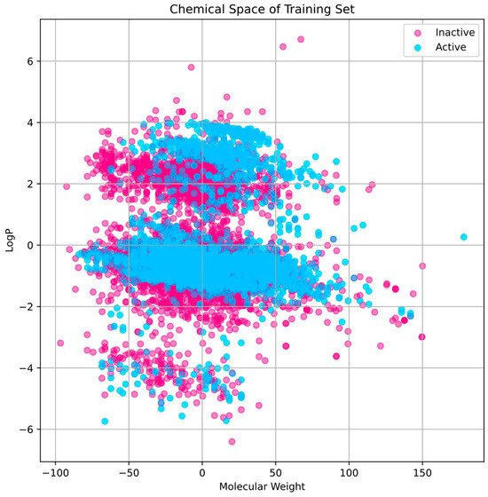
Figure 2.
Within the training set, the division of chemical space and variety. The LogP and MW are two of the characteristics that define the chemical space.
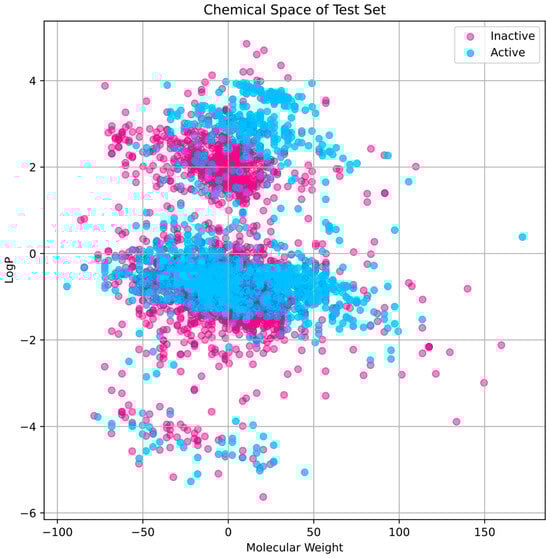
Figure 3.
Chemical space’s distribution and diversity within the test set. LogP and molecular weight are two parameters that characterize the chemical space.
In order to examine molecular similarities, we computed the Tanimoto values for the molecule pairings in our dataset. Tanimoto coefficient is an established chemoinformatics measure for assessing how similar two chemicals are based on their chemical fingerprints. For molecules, the range of the coefficients is 0 to 1 (no resemblance). Because it enables the algorithms to learn and collect a broad range of chemical properties, this diversity is advantageous for creating reliable machine-learning models. As shown in Figure 4, the histogram of the Tanimoto scores illustrates the distribution of chemical similarities between compound pairs. The wide spread of scores across the histogram indicates a broad chemical space, which is essential in preventing overfitting during model training.
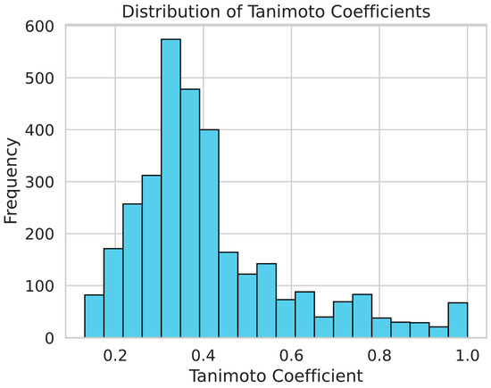
Figure 4.
The distribution of chemical similarities between pairs in our sample is depicted by the Tanimoto score histogram. The wide chemical space is indicated by the histograms, which is crucial for minimizing overfitting in the models of machine learning.
The chemicals (inactive as well as active) show a broad range of values between two primary components in both the training and test sets (Table 3). Active molecules in the training set possess a greater molecular weight and tend to be less lipophilic than inactive compounds, according to the mean values. In contrast, the standard deviation demonstrates significant variation inside every group. These results emphasize the intricate connection between a compound’s chemical properties and biological function, highlighting the need for precise prediction through the application of potent machine-learning techniques.
Table 3.
Principal components statistics summary.
3.4. Model Generation and Validation
We utilized multiple machine-learning classifiers, including kNN, SVM, RF, and NB, to classify the active inhibitors of NTRK. These models were created with Python’s sklearn module and trained on data through BindingDB. The accuracy, MCC, sensitivity, specificity, and AUC of these models were tested using several statistical measures. Table 4 illustrates how every model performed for the test set.
Table 4.
Metrics for evaluating expected model performance.
According to the findings, the RF classifier outscored all other models in every category. Specificity was 0.938892, sensitivity was 0.923408, accuracy was 0.931190, MCC was 0.862461, and AUC was 0.975943. This indicates that the RF is the most trustworthy model since it offers an exceptional combination of predicting true negatives (inactive substances) and true positives (active chemicals).
Meanwhile, the kNN model worked admirably at a comparatively high 0.902857 accuracy and an acceptable MCC of 0.809407, demonstrating its suitability as a useful substitute model for that problem. In contrast, the sensitivity of the SVM and GNB models was high, but their specificity and MCC were not as fast. Although these algorithms perform well at recognizing true positives, their rate of false positives is greater. As a consequence, although these algorithms may be helpful when overlooking a positive instance, which is costly, they are inefficient in the typical task of classification for this dataset. In terms of accuracy and MCC, the RF model outperformed prior machine-learning models deployed. It is important to remember that a model’s AUC directly affects how well it performs. As demonstrated in Figure 5, the SVM model was the next best AUC after the RF algorithm.
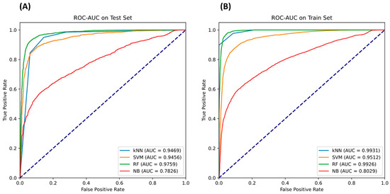
Figure 5.
The ROC-AUC curve for each classifier on the (A) test and (B) train sets.
The RF classifier was then utilized to classify the active plant chemicals that inhibit NTRK. Surprisingly, 1313 phytochemicals from a library of 9000 active compounds were screened as active against NTRK protein (Supplemental Table S4). This shows the applicability and precision of the RF classifier in this particular situation for the prediction of active chemicals.
3.5. Examining the Drug-like Ability of Active Chemicals
After determining which phytochemicals are active, we examined their drug similarity, which is an important factor in assessing prospective treatments. Using RDKit’s module named Lipinski, we determined important properties of molecules such as HBA, MW, HBD, and LogP for these active substances. The foundation of the drug-likeness standard is based on Lipinski’s Rule of Five, which states that a molecule with an MW of 500 Da, five H-bond donors, ten H-bond acceptors, and a LogP value of 5 is probably going to absorb or penetrate well. Surprisingly, 65 of the 1313 active phytochemicals met these requirements, indicating great promise for additional docking investigations and drug candidate development (Supplemental Table S5). We created a correlation matrix heatmap (Figure 6) to better understand the interactions and correlations between these chemical features. This heatmap visualizes the coefficients of correlation between every set of attributes. The intensity and correlation type are represented in this heatmap using varied colors ranging from dark red to dark blue, showing a strong negative and strong positive correlation, respectively.
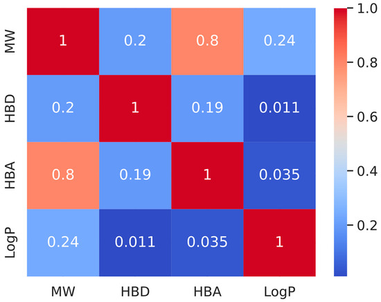
Figure 6.
The correlation matrix for molecular characteristics is shown as a heatmap. The heatmap visualizes the coefficients of correlation between each set of characteristics. The darker the hue, the greater the association.
We created a scatter matrix figure (Figure 7) to demonstrate the distribution of these drug-like features among the chosen substances. The seaborn pair plot function presents a paired connection for a collection of variables in this plot. Each point of the data shows a separate chemical inside a multidimensional universe of molecular characteristics. We may see the distribution of values for each characteristic using diagonal kernel density estimation (KDE).
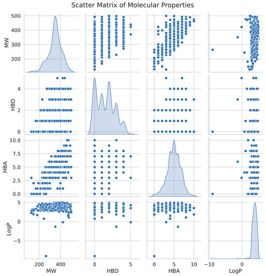
Figure 7.
Scatter matrix illustrating the distribution and correlation of key molecular properties (MW, HBD, HBA, and LogP) for active and inactive compounds, highlighting the relationships between these features and their influence on compound classification. The diagonal plots represent kernel density estimates for each property.
The scatter matrix shows substantial clusters in general, indicating that our choice of probable drug-like chemicals has comparable molecular characteristics that bond well for future pharmaceutical research. These results offer a strong basis for further experimental validation and possible therapeutic uses when paired with the machine-learning prediction results.
3.6. Analysis of Molecular Docking
We conducted comprehensive molecular docking investigations using the NTRK protein using a robust virtual screening-based technique. This screening was carried out on a wide library of 65 phytochemicals, and the five compounds with the highest binding affinity were chosen for future study (Supplemental Table S6). A control drug, Larotrectinib, was also utilized to analyze molecular docking. Gancaonin X was the complex plant chemical with a higher affinity of binding. The binding affinity of this molecule was −8.2 kcal/mol, with an RMSD of 0.565 Å. It had a significant interaction with LEU A:608, HIS A:690, and ASP A:710 residues. Next, 5-hydroxy-2-(4-methoxyphenyl)-8,8-dimethyl-2,3-dihydropyrano[2,3-h]chromen-4-one demonstrated an energy of binding −8.1 kcal/mol, and a RMSD of 2.975 Å. The residues in its interactions were LEU A:608, LEU A:611, and ILE A:616. (2S)-7-[[(2R)-3,3-dimethyloxiran-2-yl]methoxy]-5-hydroxy-2-phenyl-2,3-dihydrochromen-4-one was among the third most powerful substance, having a binding score of −8.0 kcal/mol and RMSD of 0.5 Å, primarily concerned with HIS A:690 residue. (2S)-5-hydroxy-2-(4-methoxyphenyl)-8,8-dimethyl-2,3-dihydropyrano[2,3-h]chromen-4-one, the fourth chemical was found to have an affinity of −7.9 kcal/mol and RMSD of 2.532 Å, mostly have interaction with LEU A:608, ILE A:616, HIS A:690, and ASP A:710 residues. Lastly, methyl 2-(methylamino)-5-[(3S)-1,2,3,9-tetrahydropyrrolo[2,1-b]quinazolin-3-yl]benzoate, with a binding score of −7.8 kcal/mol and RMSD of 0.014 Å, was discovered to having interaction with HIS A:690. Finally, this detailed docking study revealed distinct interactions between compounds and the NTRK protein, demonstrating they might serve as novel therapeutics (Table 5; Figure 8). The control drug, Larotrectinib, binds to NTRK with a binding affinity of −7.7 Kcal/mol and RMSD of 1.278 Å. The interacted residues were HIS A:690 and ASP A:710.
Table 5.
Docked complexes’ binding score and RMSD values.
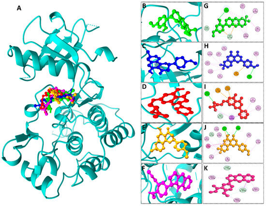
Figure 8.
(A) 3D depiction of active chemicals in conjunction with NTRK protein. 3D interaction of (B) Gancaonin X, (C) 5-hydroxy-2-(4-methoxyphenyl)-8,8-dimethyl-2,3-dihydropyrano [2,3-h]chromen-4-one, (D) (2S)-7-[[(2R)-3,3-dimethyloxiran-2-yl]methoxy]-5-hydroxy-2-phenyl-2,3-dihydrochromen-4-one, (E) (2S)-5-hydroxy-2-(4-methoxyphenyl)-8,8-dimethyl-2,3-dihydropyrano [2,3-h]chromen-4-one, and (F) methyl 2-(methylamino)-5-[(3S)-1,2,3,9-tetrahydropyrrolo [2,1-b]quinazolin-3-yl]benzoate. Two-dimensional interaction of (G) Gancaonin X, (H) 5-hydroxy-2-(4-methoxyphenyl)-8,8-dimethyl-2,3-dihydropyrano [2,3-h]chromen-4-one, (I) (2S)-7-[[(2R)-3,3-dimethyloxiran-2-yl]methoxy]-5-hydroxy-2-phenyl-2,3-dihydrochromen-4-one, (J) (2S)-5-hydroxy-2-(4-methoxyphenyl)-8,8-dimethyl-2,3-dihydropyrano [2,3-h]chromen-4-one, and (K) methyl 2-(methylamino)-5-[(3S)-1,2,3,9-tetrahydropyrrolo [2,1-b]quinazolin-3-yl]benzoate.
3.7. MD Simulation
The phytochemicals that were deemed important were reanalyzed using the Desmond software through MD simulation. Through a 100 ns molecular dynamics simulation, we observed changes over time. We monitored the structural and dynamic changes by observing the root mean square fluctuation (RMSF) and root mean square deviation (RMSD). The phytochemicals formed stable complexes with NTRK (PDB ID: 4ASZ).
3.7.1. RMSD and RMSF
To analyze the conformational dynamics of protein–ligand complexes throughout 100 ns, we conducted MD simulations. During these simulations, we calculated the RMSD and RMSF values of the top five docking complexes, focusing on the backbone atoms of the NTRK protein. The RMSD represents the average distance between the aligned protein and ligand atoms throughout the molecular docking and simulation process. Similarly, the RMSF is a statistical measurement that is comparable to the RMSD. Before calculating the RMSD and RMSF, the ligand and protein were aligned. We used an automated process with Desmond to carry out these calculations.
Figure 9 displays the RMSD plots for the top five phytochemicals. Each simulation lasted for 100 ns. Throughout the simulation, the RMSD plot for complex 1 indicated that the protein (dark cyan) exhibited a gradual increase until reaching 50 ns, after which it remained stable until the end. The ligand (brown color) displayed a mean RMSD value of 1.82 ± 0.17 Å (Figure 9A). The RMSD plot for complex 2 showed that the protein (dark cyan) demonstrated a slight elevation until 45 ns and remained constant thereafter with a mean RMSD of 0.71 ± 0.29 Å. The mean RMSD value for the ligand (brown color) was identified as 1.66 ± 0.33 Å (Figure 9C). The RMSD graph for complex 3 showed that the protein (dark cyan) exhibited a marginal rise until 63 ns, followed by a small down of 3 ns, another rise, and a consistent stability until the conclusion with the mean RMSD of 1.4 ± 0.6 Å. The mean RMSD measurement for the ligand (brown color) was noted as 1.66 ± 0.33 Å (Figure 9E). The RMSD profile for complex 4 showed that the protein (dark cyan) displayed a minor upswing until 18 ns with the mean RMSD of 1.43 ± 0.75 Å. The mean RMSD value for the ligand (brown color) was measured at 1.78 ± 0.22 Å (Figure 9G). Lastly, the RMSD plot (dark cyan) for complex 5 depicted a huge elevation at the 45 ns point. After 55 ns, the remaining were constant for the remainder of the simulation and had the mean RMSD of 1.83 ± 0.27 Å. The mean RMSD value for the ligand (brown color) was calculated as 1.71 ± 0.29 Å (Figure 9I).
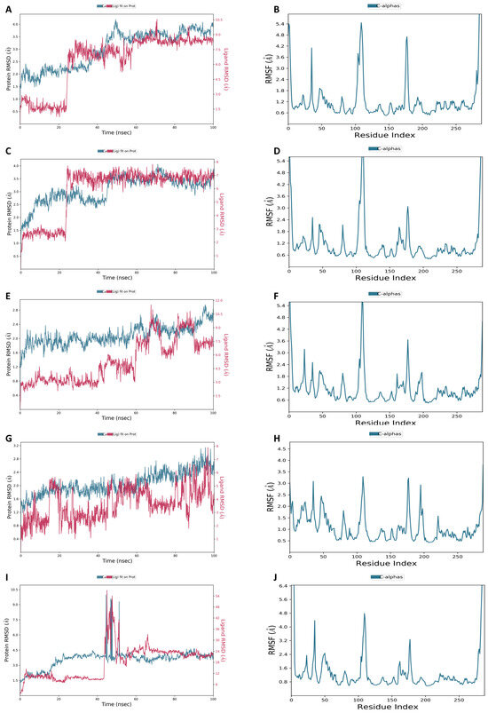
Figure 9.
RMSD and RMSF of (A,B) Gancaonin X, (C,D) 5-hydroxy-2-(4-methoxyphenyl)-8,8-dimethyl-2,3-dihydropyrano [2,3-h]chromen-4-one, (E,F) (2S)-7-[[(2R)-3,3-dimethyloxiran-2-yl]methoxy]-5-hydroxy-2-phenyl-2,3-dihydrochromen-4-one, (G,H) (2S)-5-hydroxy-2-(4-methoxyphenyl)-8,8-dimethyl-2,3-dihydropyrano [2,3-h]chromen-4-one, and (I,J) methyl 2-(methylamino)-5-[(3S)-1,2,3,9-tetrahydropyrrolo [2,1-b]quinazolin-3-yl]benzoate, respectively.
In addition, the RMSF metrics were used to determine the fluctuation in residues along the protein chain. The peaks of the RMSF indicate the areas of the protein where residues experience the highest level of fluctuation throughout the simulation trajectory. While RMSD measures the average positional distance of the entire system, RMSF calculates the flexibility of individual residues. It is a useful tool for assessing how much a particular residue moves during the simulation. Figure 9 displays the RMSF peaks of the docked complexes. These peaks demonstrate that the protein remains stable during ligand binding. Furthermore, the RMSF peaks of all five complexes show that the protein remains stable during the binding process with the ligands (Figure 9B,D,F,H,J).
3.7.2. Radius of Gyration (Rg) and Solvent Accessible Surface Area (SASA)
The MD simulations were performed for four samples, of which the Rg and SADA properties were analyzed. For complex 1, the Rg gradually increased to 25 ns, but after that, it suddenly became stable, except for a bit down at 43 ns and 88 ns. The SASA was slightly up and down through time (Figure 10A). For complex 2, the Rg stabilized throughout the time, but SASA fluctuated up by 23 ns (Figure 10B). For complex 3, Rg and SADA fluctuated at 38 ns and 75 ns, respectively (Figure 10C). For complex 4, both the Rg and SASA were almost stable throughout the time (Figure 10D). Finally, the Rg of complex 5 was slightly down from 25–35 ns and stabilized for the other time, but the SASA fluctuated highly up from 22–68 ns (Figure 10E).
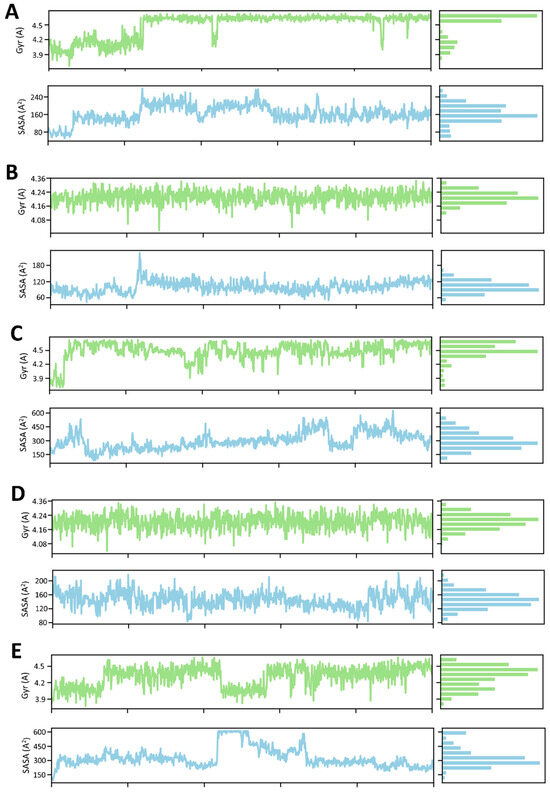
Figure 10.
The time frame evaluation against the radius of gyration (Rg) and solvent accessible surface area (SASA) of (A) Gancaonin X, (B) 5-hydroxy-2-(4-methoxyphenyl)-8,8-dimethyl-2,3-dihydropyrano [2,3-h]chromen-4-one, (C) (2S)-7-[[(2R)-3,3-dimethyloxiran-2-yl]methoxy]-5-hydroxy-2-phenyl-2,3-dihydrochromen-4-one, (D) (2S)-5-hydroxy-2-(4-methoxyphenyl)-8,8-dimethyl-2,3-dihydropyrano [2,3-h]chromen-4-one, and (E) methyl 2-(methylamino)-5-[(3S)-1,2,3,9-tetrahydropyrrolo [2,1-b]quinazolin-3-yl]benzoate.
3.7.3. Protein–Ligand Interaction
To accurately predict the binding pocket of docked compounds to the target protein’s binding site, it is necessary to have atomic-level information. In our analysis using MD simulation for 100 ns, we carefully examined various intermolecular interactions, including H-bonds, H2O bridges, hydrophobic interactions, and ionic interactions. This allowed us to evaluate the critical modes effectively. The data showed that the Gancaonin X made a strong H-bonding with ASN_610, VAL_689, HIS_690, and ARG_691. It showed hydrophobic interactions with LEU_607, LEU_608, LEU_611, ILE_616, VAL_617, PHE_633, LEU_683, PHE_688, VAL_689, HIS_690, ARG_691, and ILE_708. It also showed ionic strength with LYS_588, ARG_603, GLU_604, GLU_606, ASN_610, HIS_687, VAL_689, ARG_691, ASP_692, ASP_710, and ARG_715. All the other compounds also have strong H-bonding, hydrophobic interactions, and ionic strength, as depicted in Figure 11.
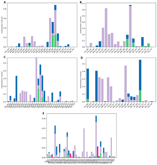
Figure 11.
Protein–ligand interaction profiles for (A) Gancaonin X, (B) 5-hydroxy-2-(4-methoxyphenyl)-8,8-dimethyl-2,3-dihydropyrano [2,3-h]chromen-4-one, (C) (2S)-7-[[(2R)-3,3-dimethyloxiran-2-yl]methoxy]-5-hydroxy-2-phenyl-2,3-dihydrochromen-4-one, (D) (2S)-5-hydroxy-2-(4-methoxyphenyl)-8,8-dimethyl-2,3-dihydropyrano [2,3-h]chromen-4-one, and (E) methyl 2-(methylamino)-5-[(3S)-1,2,3,9-tetrahydropyrrolo [2,1-b]quinazolin-3-yl]benzoate.
4. Discussion
NSCLC is primarily caused by smoking and occupational exposures to carcinogens such as asbestos, radon, and air pollution. Other risk factors include genetic predisposition, with some individuals having a higher risk due to family history or inherited genetic mutations [5]. Despite substantial improvements in understanding the disorder’s pathogenesis, effective therapy choices for drug-resistant NSCLC remain limited. As a result, the discovery of innovative, effective NSCLC treatment techniques is critical. NTRK proteins, transmembrane proteins that are members of the family of TRK receptors, are essential for the growth of cells and survival. These consist of TRKA, TRKB, and TRKC, which are translated by the NTRK1, NTRK2, and NTRK3 genes, respectively [62].
Advances in CADD have transformed the traditional design of novel medications that target particular proteins such as NTRK. CADD provides a speedy and accurate approach for screening large phytochemicals libraries, which can accelerate the identification and progress of new NTRK-targeting therapeutic drugs, therefore considerably altering NSCLC therapy. This strategy has been further enhanced by the application of machine-learning approaches, which offer an efficient means of differentiating between possible inactive and active compounds against the target protein. The goal of current research is to use the machine-learning classifier’s power to improve the process of drug discovery, with a specific emphasis on the discovery of novel NTRK protein inhibitors. The focus on machine learning increases virtual screening’s accuracy but also reduces the frequency of false-positive results, considerably increasing the general effectiveness and precision of drug development efforts. Machine learning is becoming more important in contemporary medicinal chemistry as it enhances the sophistication and capacities of the drug discovery process.
In the current investigation, a comprehensive dataset of 12,178 compounds was used, including 5178 known active drugs against NTRK and 7000 decoys. After identifying active and inactive chemicals, it was crucial to understand the qualities or characteristics that make some compounds efficient against the NTRK protein in the therapy of NSCLC. We employed a feature extraction and selection strategy that involved looking at physicochemical characteristics, structural fingerprints, and topological descriptors. These important properties in the process of drug development describe the reliability, reactivity, and contact of the chemical with the target protein.
PCA was utilized to preserve the variance while simplifying our multidimensional dataset. This approach provided insightful information about the fundamental elements that influence the activity of compounds. By following PCA, we created machine-learning models utilizing the selected features as input, employing the KNN, SVM, and RF algorithms. Every model was trained and verified to differentiate between inactive and active substances using the carefully selected dataset. These models’ accuracy, F1-score, precision, recall, and AUC-ROC were tested.
When predicting active chemicals, the RF model performed better than the others because of its ability to deal with high-dimensional data and take into consideration interaction effects while avoiding overfitting. The RF classifier, in particular, provides significant features, demonstrating which factors were most significant in determining whether a molecule was inactive or active. These feature-related data are crucial in defining the properties required for a chemical to be active against the NTRK protein.
The RF classifier was used to evaluate a library of 9000 phytochemicals after establishing the most reliable model, giving 1313 compounds expected to be active against the NTRK protein. As a result, there is a wide pool of potential pharmaceutical options for the treatment of NSCLC. These 1313 compounds were more studied by employing Lipinski’s Rule of Five, with a specific focus on their drug-likeness. This principle is widely used and frequently followed in the drug development field, and it is used to predict a compound’s oral bioavailability. We reduced the number of chemicals in our collection using Lipinski’s Rule to 65, which satisfied these requirements, and we believe the human body will effectively absorb these compounds.
Using molecular docking, the interactions between these 65 chemicals and the NTRK protein were simulated. This study revealed five chemicals with a high affinity for binding to the NTRK protein, which could result in the creation of innovative treatments for NSCLC. The phytochemicals with highest binding affinity were Gancaonin X, 5-hydroxy-2-(4-methoxyphenyl)-8,8-dimethyl-2,3-dihydropyrano[2,3-h]chromen-4-one, (2S)-7-[[(2R)-3,3-dimethyloxiran-2-yl]methoxy]-5-hydroxy-2-phenyl-2,3-dihydrochromen-4-one, (2S)-5-hydroxy-2-(4-methoxyphenyl)-8,8-dimethyl-2,3-dihydropyrano[2,3-h]chromen-4-one, and methyl 2-(methylamino)-5-[(3S)-1,2,3,9-tetrahydropyrrolo[2,1-b]quinazolin-3-yl]benzoate.
The molecular dynamics (MD) simulations conducted in this study provide valuable insights into the dynamic behavior of phytochemical-NTRK complexes over a 100 ns trajectory. The analysis of root mean square deviation (RMSD) and root mean square fluctuation (RMSF) revealed distinct patterns in the conformational dynamics of the top five docking complexes. Notably, the RMSD plots illustrated the stability of protein–ligand interactions, with fluctuations in the ligand’s position within acceptable ranges. Furthermore, the RMSF metrics highlighted specific regions of the protein chain experiencing fluctuation, emphasizing the overall stability of the protein–ligand complexes.
The evaluation of the radius of gyration (Rg) and solvent-accessible surface area (SASA) provided additional dimensions to the understanding of complex dynamics. While Rg exhibited stability in most complexes, SASA fluctuations indicated dynamic solvent accessibility. The time-dependent analysis of Rg and SASA for each complex contributed to a comprehensive characterization of their structural dynamics.
The exploration of protein–ligand interactions through MD simulations elucidated critical intermolecular forces, including hydrogen bonding, hydrophobic interactions, and ionic interactions. Gancaonin X, for instance, demonstrated strong and sustained interactions with specific amino acid residues, suggesting its potential as a stable binding ligand. These findings deepen our understanding of the dynamic behavior and binding mechanisms of phytochemical-NTRK complexes, providing essential information for future drug development efforts targeting neurotrophic receptor kinases.
Samad et al. combined machine learning along with virtual screening to identify a possible inhibitor of SARS-CoV-2 for 3CLpro protein. Alshehri [21] also utilized machine learning-based methods for the identification of S100B protein-related key inhibitors for the treatment of epilepsy. To summarize, our findings have significant significance for the area of drug development, particularly in the search for NSCLC treatments. We were able to scan a vast library of phytochemicals using a machine learning-based method and to find possible lead compounds that interact with the NTRK protein, one of the main targets of NSCLC. This personalized technique might result in the creation of such drugs, which can alter the disease’s core processes instead of just handling the symptoms. Moreover, by using computational methodologies to identify interesting candidates for further inquiry, this work contributes to the simplification of the drug development procedure, which has historically required a lot of time and resources.
Modern computational drug discovery methods support our research since it follows other studies that use machine learning-based virtual screening to discover NSCLC inhibitors. Virtual screening methodologies combining traditional methods with machine learning have proven successful for PDGFR inhibitor discovery in NSCLC performed by Reddy et al. (2025) [63]. The research by Cai et al. (2024) demonstrated how generative deep learning models can screen STAT3 phosphorylation inhibitors as predictive prospective agents for NSCLC treatment through virtual methods [64].
Our research used machine learning integrated virtual screening to find numerous drugs with proven effectiveness in the treatment of NSCLC. The numerous pharmacological features of the substances anticipated in this work, such as anti-inflammatory and anti-cancer activities, highlight their capacities for further research into their influence on cancer diseases. To prove efficacy, safety, and appropriate use, as with any prospective treatment, extensive scientific inquiry would be required.
Furthermore, there are important constraints, such as the dependence on the caliber and range of our data gathering, which is a major constraint. Despite using a huge plant chemical library, the caliber and variety of the training dataset affect our machine-learning algorithms’ effectiveness. As a result, any bias or lack of variation in the prediction findings might restrict the results of the predictions. Moreover, the interactions that are disclosed by the in silico methods are hypothetical and need to be confirmed by in vitro and in vivo experiments. To evaluate their therapeutic value, these discoveries will be required to be investigated more in cell-based assays as well as animal models. Studies on pharmacokinetics and pharmacodynamics are also necessary to guarantee the effectiveness and security of the substances detected in humans. Future work on this project could include adding more phytochemicals to the library and including more varied datasets to test and train our machine-learning algorithms. Furthermore, novel treatments for NSCLC may be developed as a result of a better comprehension of the molecular mechanisms behind the interactions between the discovered chemicals and the NTRK protein. Lastly, the results of this investigation may inspire comparable research methodologies for other illnesses, leading to a rise in the application of machine learning in drug development processes across many therapeutic domains.
5. Conclusions
The latest work has enhanced our comprehension of the NTRK protein as a promising therapeutic target in NSCLC. Our work has expedited the arduous and time-consuming process of pharmaceutical creation by using the capabilities of machine-learning classifiers and CADD. We utilized an extensive dataset of chemicals to create and verify machine-learning classifiers that effectively distinguished between inactive and active chemicals targeting the NTRK protein (TRKB). The Random Forest model had superior performance compared to the other algorithms employed, demonstrating exceptional forecast accuracy and offering insightful information about the significance of features. After using that method, a comprehensive collection of phytochemicals was examined, leading to the identification of 1313 compounds that are anticipated to have activity against NTRK. This list was reduced to 65 compounds with desired drug-like properties using Lipinski’s Rule of Five. Five phytochemicals with remarkable binding affinities to the NTRK protein were identified using molecular docking of these 65 compounds, suggesting that they may be promising therapeutic approaches against NSCLC. The 100 ns molecular dynamics simulations unveiled the stable nature of the top five phytochemical-NTRK complexes, as evidenced by consistent RMSD and RMSF profiles. Additionally, the exploration of Rg and SASA dynamics highlighted nuanced structural changes, while the detailed analysis of protein–ligand interactions illuminated key molecular forces governing stable binding interactions. Overall, our research demonstrates how machine learning and drug design together could expedite the creation of new drugs. Although our results are promising, we point out that more validation is needed for the suggested CAAD strategy. As a result, we emphasized throughout our conversation the significance of conducting more research with a variety of datasets and conditions. Although NSCLC and the NTRK protein were the focus of our attention, we believe that other diseases and targets could benefit from the use of our technique. These kinds of initiatives may encourage the creation of targeted and effective treatments, improving the quality of life for a great number of NSCLC patients worldwide.
Supplementary Materials
The following supporting information can be downloaded at: https://www.mdpi.com/article/10.3390/cryst15050383/s1.
Author Contributions
Conceptualization, Z.S.A.S.; Data curation, Z.S.A.S.; Formal analysis, Z.S.A.S.; Funding acquisition, Z.S.A.S.; Methodology, F.F.A.; Project administration, F.F.A.; Resources, Z.S.A.S.; Validation, F.F.A.; Visualization, Z.S.A.S.; Writing—original draft, Z.S.A.S.; Writing—review and editing, F.F.A. All authors have read and agreed to the published version of the manuscript.
Funding
This research received no external funding.
Data Availability Statement
The data presented in this study are available within the article.
Acknowledgments
The researcher would like to thank the Deanship of Scientific Research, Shaqra University, for funding the publication of this project.
Conflicts of Interest
The author declares no conflicts of interest.
References
- Goldstraw, P.; Ball, D.; Jett, J.R.; Le Chevalier, T.; Lim, E.; Nicholson, A.G.; Shepherd, F.A. Non-small-cell lung cancer. Lancet 2011, 378, 1727–1740. [Google Scholar] [CrossRef] [PubMed]
- Jadhav, S.P. Introduction to lung diseases. Target. Cell. Signal. Pathw. Lung Dis. 2021, 1–25. [Google Scholar]
- Rekhtman, N.; Travis, W.D. Large no more: The journey of pulmonary large cell carcinoma from common to rare entity. J. Thorac. Oncol. 2019, 14, 1125–1127. [Google Scholar] [CrossRef]
- Simoff, M.J.; Lally, B.; Slade, M.G.; Goldberg, W.G.; Lee, P.; Michaud, G.C.; Wahidi, M.M.; Chawla, M. Symptom management in patients with lung cancer: Diagnosis and management of lung cancer: American College of Chest Physicians evidence-based clinical practice guidelines. Chest 2013, 143, e455S–e497S. [Google Scholar] [CrossRef]
- Shankar, A.; Dubey, A.; Saini, D.; Singh, M.; Prasad, C.P.; Roy, S.; Bharati, S.J.; Rinki, M.; Singh, N.; Seth, T.; et al. Environmental and occupational determinants of lung cancer. Transl. Lung Cancer Res. 2019, 8, S31. [Google Scholar] [CrossRef] [PubMed]
- Sarode, P.; Mansouri, S.; Karger, A.; Schaefer, M.B.; Grimminger, F.; Seeger, W.; Savai, R. Epithelial cell plasticity defines heterogeneity in lung cancer. Cell. Signal. 2020, 65, 109463. [Google Scholar] [CrossRef]
- Drilon, A.; Rekhtman, N.; Ladanyi, M.; Paik, P. Squamous-cell carcinomas of the lung: Emerging biology, controversies, and the promise of targeted therapy. Lancet Oncol. 2012, 13, e418–e426. [Google Scholar] [CrossRef]
- Mustafa, M.; Azizi, A.J.; IIIzam, E.; Nazirah, A.; Sharifa, S.; Abbas, S. Lung cancer: Risk factors, management, and prognosis. IOSR J. Dent. Med. Sci. 2016, 15, 94–101. [Google Scholar] [CrossRef]
- Samet, J.M.; Avila-Tang, E.; Boffetta, P.; Hannan, L.M.; Olivo-Marston, S.; Thun, M.J.; Rudin, C.M. Lung cancer in never smokers: Clinical epidemiology and environmental risk factors. Clin. Cancer Res. 2009, 15, 5626–5645. [Google Scholar] [CrossRef]
- Amatu, A.; Sartore-Bianchi, A.; Bencardino, K.; Pizzutilo, E.G.; Tosi, F.; Siena, S. Tropomyosin receptor kinase (TRK) biology and the role of NTRK gene fusions in cancer. Ann. Oncol. 2019, 30, viii5–viii15. [Google Scholar] [CrossRef]
- Hsiao, S.J.; Zehir, A.; Sireci, A.N.; Aisner, D.L. Detection of tumor NTRK gene fusions to identify patients who may benefit from tyrosine kinase (TRK) inhibitor therapy. J. Mol. Diagn. 2019, 21, 553–571. [Google Scholar] [CrossRef]
- Chevallier, M.; Borgeaud, M.; Addeo, A.; Friedlaender, A. Oncogenic driver mutations in non-small cell lung cancer: Past, present and future. World J. Clin. Oncol. 2021, 12, 217. [Google Scholar] [CrossRef]
- Vaughn, C.P.; Costa, J.L.; Feilotter, H.E.; Petraroli, R.; Bagai, V.; Rachiglio, A.M.; Marino, F.Z.; Tops, B.; Kurth, H.M.; Sakai, K.; et al. Simultaneous detection of lung fusions using a multiplex RT-PCR next-generation sequencing-based approach: A multi-institutional research study. BMC Cancer 2018, 18, 828. [Google Scholar] [CrossRef] [PubMed]
- Demetri, G.D.; De Braud, F.; Drilon, A.; Siena, S.; Patel, M.R.; Cho, B.C.; Liu, S.V.; Ahn, M.-J.; Chiu, C.-H.; Lin, J.J.; et al. Updated integrated analysis of the efficacy and safety of entrectinib in patients with NTRK fusion-positive solid tumors. Clin. Cancer Res. 2022, 28, 1302–1312. [Google Scholar] [CrossRef]
- Patel, L.; Shukla, T.; Huang, X.; Ussery, D.W.; Wang, S. Machine learning methods in drug discovery. Molecules 2020, 25, 5277. [Google Scholar] [CrossRef] [PubMed]
- Cuny, C.; Friedrich, A.; Kozytska, S.; Layer, F.; Nübel, U.; Ohlsen, K.; Strommenger, B.; Walther, B.; Wieler, L.; Witte, W. Emergence of methicillin-resistant Staphylococcus aureus (MRSA) in different animal species. Int. J. Med. Microbiol. 2010, 300, 109–117. [Google Scholar] [CrossRef] [PubMed]
- Noor, F.; Noor, A.; Ishaq, A.R.; Farzeen, I.; Saleem, M.H.; Ghaffar, K.; Aslam, M.F.; Aslam, S.; Chen, J.T. Recent advances in diagnostic and therapeutic approaches for breast cancer: A comprehensive review. Curr. Pharm. Des. 2021, 27, 2344–2365. [Google Scholar] [CrossRef]
- Tripathi, A.; Misra, K.; Dhanuka, R.; Singh, J.P. Artificial intelligence in accelerating drug discovery and development. Recent Pat. Biotechnol. 2023, 17, 9–23. [Google Scholar] [CrossRef]
- Yang, J.; Cai, Y.; Zhao, K.; Xie, H.; Chen, X. Concepts and applications of chemical fingerprint for hit and lead screening. Drug Discov. Today 2022, 27, 103356. [Google Scholar] [CrossRef]
- Samad, A.; Ajmal, A.; Mahmood, A.; Khurshid, B.; Li, P.; Jan, S.M.; Rehman, A.U.; He, P.; Abdalla, A.N.; Umair, M.; et al. Identification of novel inhibitors for SARS-CoV-2 as therapeutic options using machine learning-based virtual screening, molecular docking and MD simulation. Front. Mol. Biosci. 2023, 10, 1060076. [Google Scholar] [CrossRef]
- Alshehri, F.F. Integrated virtual screening, molecular modeling and machine learning approaches revealed potential natural inhibitors for epilepsy. Saudi Pharm. J. 2023, 31, 101835. [Google Scholar] [CrossRef] [PubMed]
- Almatroudi, A. Integrative Machine Learning, Virtual Screening, and Molecular Modeling for BacA-Targeted Anti-Biofilm Drug Discovery Against Staphylococcal Infections. Crystals 2024, 14, 1057. [Google Scholar] [CrossRef]
- Zulfat, M.; Hakami, M.A.; Hazazi, A.; Mahmood, A.; Khalid, A.; Alqurashi, R.S.; Abdalla, A.N.; Huh, J.; Wadooda, A.; Huang, X. Identification of novel NLRP3 inhibitors as therapeutic options for epilepsy by machine learning-based virtual screening, molecular docking and biomolecular simulation studies. Heliyon 2024, 10, e34410. [Google Scholar] [CrossRef]
- Liu, T.; Lin, Y.; Wen, X.; Jorissen, R.N.; Gilson, M.K. BindingDB: A web-accessible database of experimentally determined protein–ligand binding affinities. Nucleic Acids Res. 2007, 35, D198–D201. [Google Scholar] [CrossRef] [PubMed]
- Mysinger, M.M.; Carchia, M.; Irwin, J.J.; Shoichet, B.K. Directory of useful decoys, enhanced (DUD-E): Better ligands and decoys for better benchmarking. J. Med. Chem. 2012, 55, 6582–6594. [Google Scholar] [CrossRef] [PubMed]
- McKinney, W.; Team, P.D. Pandas-Powerful python data analysis toolkit. Pandas—Powerful Python Data Anal. Toolkit 2015, 1625. [Google Scholar]
- Chawla, N.V.; Bowyer, K.W.; Hall, L.O.; Kegelmeyer, W.P. SMOTE: Synthetic minority over-sampling technique. J. Artif. Intell. Res. 2002, 16, 321–357. [Google Scholar] [CrossRef]
- Pedregosa, F.; Varoquaux, G.; Gramfort, A.; Michel, V.; Thirion, B.; Grisel, O.; Blondel, M.; Prettenhofer, P.; Weiss, R.; Dubourg, V.; et al. Scikit-learn: Machine learning in Python. J. Mach. Learn. Res. 2011, 12, 2825–2830. [Google Scholar]
- Bento, A.P.; Hersey, A.; Félix, E.; Landrum, G.; Gaulton, A.; Atkinson, F.; Bellis, L.J.; De Veij, M.; Leach, A.R. An open source chemical structure curation pipeline using RDKit. J. Cheminform. 2020, 12, 51. [Google Scholar] [CrossRef]
- Godden, J.W.; Xue, L.; Bajorath, J. Combinatorial preferences affect molecular similarity/diversity calculations using binary fingerprints and Tanimoto coefficients. J. Chem. Inf. Comput. Sci. 2000, 40, 163–166. [Google Scholar] [CrossRef]
- Orosz, Á.; Héberger, K.; Rácz, A. Comparison of descriptor-and fingerprint sets in machine learning models for ADME-Tox targets. Front. Chem. 2022, 10, 852893. [Google Scholar] [CrossRef]
- Sharma, A.; Lal, S.P. Tanimoto based similarity measure for intrusion detection system. J. Inf. Secur. 2011, 2, 195–201. [Google Scholar] [CrossRef][Green Version]
- Alexander, N.; Woetzel, N.; Meiler, J. Bcl::Cluster: A method for clustering biological molecules coupled with visualization in the Pymol Molecular Graphics System. In Proceedings of the 2011 IEEE 1st International Conference on Computational Advances in Bio and Medical Sciences, ICCABS 2011, Orlando, FL, USA, 3–5 February 2011; pp. 13–18. [Google Scholar] [CrossRef]
- Maćkiewicz, A.; Ratajczak, W. Principal components analysis (PCA). Comput. Geosci. 1993, 19, 303–342. [Google Scholar] [CrossRef]
- Groth, D.; Hartmann, S.; Klie, S.; Selbig, J. Principal components analysis. Comput. Toxicol. 2013, 2, 527–547. [Google Scholar]
- Huang, S.; Cai, N.; Pacheco, P.P.; Narrandes, S.; Wang, Y.; Xu, W. Applications of support vector machine (SVM) learning in cancer genomics. Cancer Genom. Proteom. 2018, 15, 41–51. [Google Scholar]
- Adugna, T.; Xu, W.; Fan, J. Comparison of random forest and support vector machine classifiers for regional land cover mapping using coarse resolution FY-3C images. Remote Sens. 2022, 14, 574. [Google Scholar] [CrossRef]
- Peterson, L.E. K-nearest neighbor. Scholarpedia 2009, 4, 1883. [Google Scholar] [CrossRef]
- Pandya, V.J. Comparing handwritten character recognition by AdaBoostClassifier and KNeighborsClassifier. In Proceedings of the 2016 8th International Conference on Computational Intelligence and Communication Networks (CICN), Tehri, India, 23–25 December 2016; pp. 271–274. [Google Scholar]
- Metsis, V.; Androutsopoulos, I.; Paliouras, G. Spam filtering with naive bayes-which naive bayes? In Proceedings of the CEAS 2006—The Third Conference on Email and Anti-Spam, Mountain View, CA, USA, 27–28 July 2006; pp. 28–69. [Google Scholar]
- Belgiu, M.; Drăguţ, L. Random forest in remote sensing: A review of applications and future directions. ISPRS J. Photogramm. Remote Sens. 2016, 114, 24–31. [Google Scholar] [CrossRef]
- Qi, Y. Random forest for bioinformatics. Ensemble Mach. Learn. Methods Appl. 2012, 307–323. [Google Scholar]
- Walsh, I.; Fishman, D.; Garcia-Gasulla, D.; Titma, T.; Pollastri, G.; ELIXIR Machine Learning Focus Group; Harrow, J.; Psomopoulos, F.E.; Tosatto, S.C.E. DOME: Recommendations for supervised machine learning validation in biology. Nat. Methods 2021, 18, 1122–1127. [Google Scholar] [CrossRef]
- Burzykowski, T.; Geubbelmans, M.; Rousseau, A.-J.; Valkenborg, D. Validation of machine learning algorithms. Am. J. Orthod. Dentofac. Orthop. 2023, 164, 295–297. [Google Scholar] [CrossRef] [PubMed]
- Jolly, K. Machine Learning with Scikit-Learn Quick Start Guide: Classification, Regression, and Clustering Techniques in Python; Packt Publishing Ltd.: Birmingham, UK, 2018. [Google Scholar]
- Carrington, A.M.; Manuel, D.G.; Fieguth, P.W.; Ramsay, T.; Osmani, V.; Wernly, B.; Bennett, C.; Hawken, S.; McInnes, M.; Magwood, O.; et al. Deep ROC analysis and AUC as balanced average accuracy to improve model selection, understanding and interpretation. arXiv 2021, arXiv:2103.11357. [Google Scholar]
- Majnik, M.; Bosnić, Z. ROC analysis of classifiers in machine learning: A survey. Intell. Data Anal. 2013, 17, 531–558. [Google Scholar] [CrossRef]
- Zweig, M.H.; Campbell, G. Receiver-operating characteristic (ROC) plots: A fundamental evaluation tool in clinical medicine. Clin. Chem. 1993, 39, 561–577. [Google Scholar] [CrossRef]
- Pilgrim, M. Serializing Python Objects. In Dive Into Python 3; Springer: Berlin/Heidelberg, Germany, 2009; pp. 205–223. [Google Scholar]
- Kim, S.; Chen, J.; Cheng, T.; Gindulyte, A.; He, J.; He, S.; Li, Q.; Shoemaker, B.A.; Thiessen, P.A.; Yu, B.; et al. PubChem 2019 update: Improved access to chemical data. Nucleic Acids Res. 2019, 47, D1102–D1109. [Google Scholar] [CrossRef]
- Gaulton, A.; Bellis, L.J.; Bento, A.P.; Chambers, J.; Davies, M.; Hersey, A.; Light, Y.; McGlinchey, S.; Michalovich, D.; Al-Lazikani, B.; et al. ChEMBL: A large-scale bioactivity database for drug discovery. Nucleic Acids Res. 2012, 40, D1100–D1107. [Google Scholar] [CrossRef]
- Irwin, J.J.; Shoichet, B.K. ZINC—A free database of commercially available compounds for virtual screening. J. Chem. Inf. Model. 2005, 45, 177–182. [Google Scholar] [CrossRef]
- Chen, X.; Li, H.; Tian, L.; Li, Q.; Luo, J.; Zhang, Y. Analysis of the physicochemical properties of acaricides based on Lipinski’s rule of five. J. Comput. Biol. 2020, 27, 1397–1406. [Google Scholar] [CrossRef]
- Sussman, J.L.; Lin, D.; Jiang, J.; Manning, N.O.; Prilusky, J.; Ritter, O.; Abola, E.E. Protein Data Bank (PDB): Database of three-dimensional structural information of biological macromolecules. Acta Crystallogr. Sect. D Biol. Crystallogr. 1998, 54, 1078–1084. [Google Scholar] [CrossRef]
- Headquarters, A.C. Discovery Studio Life Science Modeling and Simulations. Res. Net. 2008, 1–8. [Google Scholar]
- Hong, D.S.; DuBois, S.G.; Kummar, S.; Farago, A.F.; Albert, C.M.; Rohrberg, K.S.; van Tilburg, C.M.; Nagasubramanian, R.; Berlin, J.D.; Federman, N.; et al. Larotrectinib in patients with TRK fusion-positive solid tumours: A pooled analysis of three phase 1/2 clinical trials. Lancet Oncol. 2020, 21, 531–540. [Google Scholar] [CrossRef]
- Dallakyan, S.; Olson, A.J. Small-molecule library screening by docking with PyRx. Methods Mol. Biol. 2015, 1263, 243–250. [Google Scholar] [CrossRef]
- Trott, O.; Olson, A.J. AutoDock Vina: Improving the speed and accuracy of docking with a new scoring function, efficient optimization, and multithreading. J. Comput. Chem. 2010, 31, 455–461. [Google Scholar] [CrossRef]
- Mohapatra, R.K.; Mahal, A.; Ansari, A.; Kumar, M.; Guru, J.P.; Sarangi, A.K.; Abdou, A.; Mishra, S.; Aljeldah, M.; AlShehail, B.M.; et al. Comparison of the binding energies of approved mpox drugs and phytochemicals through molecular docking, molecular dynamics simulation, and ADMET studies: An in silico approach. J. Biosaf. Biosecur. 2023, 5, 118–132. [Google Scholar] [CrossRef]
- Papavasileiou, K.D.; Moultos, O.A.; Economou, I.G. Predictions of water/oil interfacial tension at elevated temperatures and pressures: A molecular dynamics simulation study with biomolecular force fields. Fluid Phase Equilib. 2018, 476, 30–38. [Google Scholar] [CrossRef]
- Rajamanikandan, S.; Jeyakanthan, J.; Srinivasan, P. Molecular docking, molecular dynamics simulations, computational screening to design quorum sensing inhibitors targeting LuxP of Vibrio harveyi and its biological evaluation. Appl. Biochem. Biotechnol. 2017, 181, 192–218. [Google Scholar] [CrossRef] [PubMed]
- Khotskaya, Y.B.; Holla, V.R.; Farago, A.F.; Shaw, K.R.M.; Meric-Bernstam, F.; Hong, D.S. Targeting TRK family proteins in cancer. Pharmacol. Ther. 2017, 173, 58–66. [Google Scholar] [CrossRef]
- Reddy, S.K.; Reddy, S.V.G.; Basha, S.H. Discovery of novel PDGFR inhibitors targeting non-small cell lung cancer using a multistep machine learning assisted hybrid virtual screening approach. RSC Adv. 2025, 15, 851–869. [Google Scholar] [CrossRef]
- Cai, W.; Jiang, B.; Yin, Y.; Ma, L.; Li, T.; Chen, J. Identification of STAT3 phosphorylation inhibitors using generative deep learning, virtual screening, molecular dynamics simulations, and biological evaluation for non-small cell lung cancer therapy. Mol. Divers. 2024, 1–17. [Google Scholar] [CrossRef]


Disclaimer/Publisher’s Note: The statements, opinions and data contained in all publications are solely those of the individual author(s) and contributor(s) and not of MDPI and/or the editor(s). MDPI and/or the editor(s) disclaim responsibility for any injury to people or property resulting from any ideas, methods, instructions or products referred to in the content. |
© 2025 by the authors. Licensee MDPI, Basel, Switzerland. This article is an open access article distributed under the terms and conditions of the Creative Commons Attribution (CC BY) license (https://creativecommons.org/licenses/by/4.0/).