Thermomechanical Modeling of Amorphous Glassy Polymer Undergoing Large Viscoplastic Deformation: 3-Points Bending and Gas-Blow Forming


Abstract
:1. Introduction
2. Results
- the thermal deformation is assumed to be an isotropic thermal expansion, i.e., , where denotes the second-order identity tensor.
2.1. Hyperelasticity
2.2. Viscoplastic Flow Rule
2.3. Strain Softening
2.4. Strain Hardening
2.5. Criterion for Viscoplasticity
2.6. Temperature Evolution
3. Calibration of the Model Parameters
3.1. 1D Version of the Constitutive Equations
3.2. Model Parameter Calibration
- The reference elastic modulus was determined from the experimental stress-strain response at the reference temperature . The model parameter was determined from the experimental stress-strain response at different temperatures. Poisson’s ratio and the thermal expansion coefficient were obtained from the literature [26].
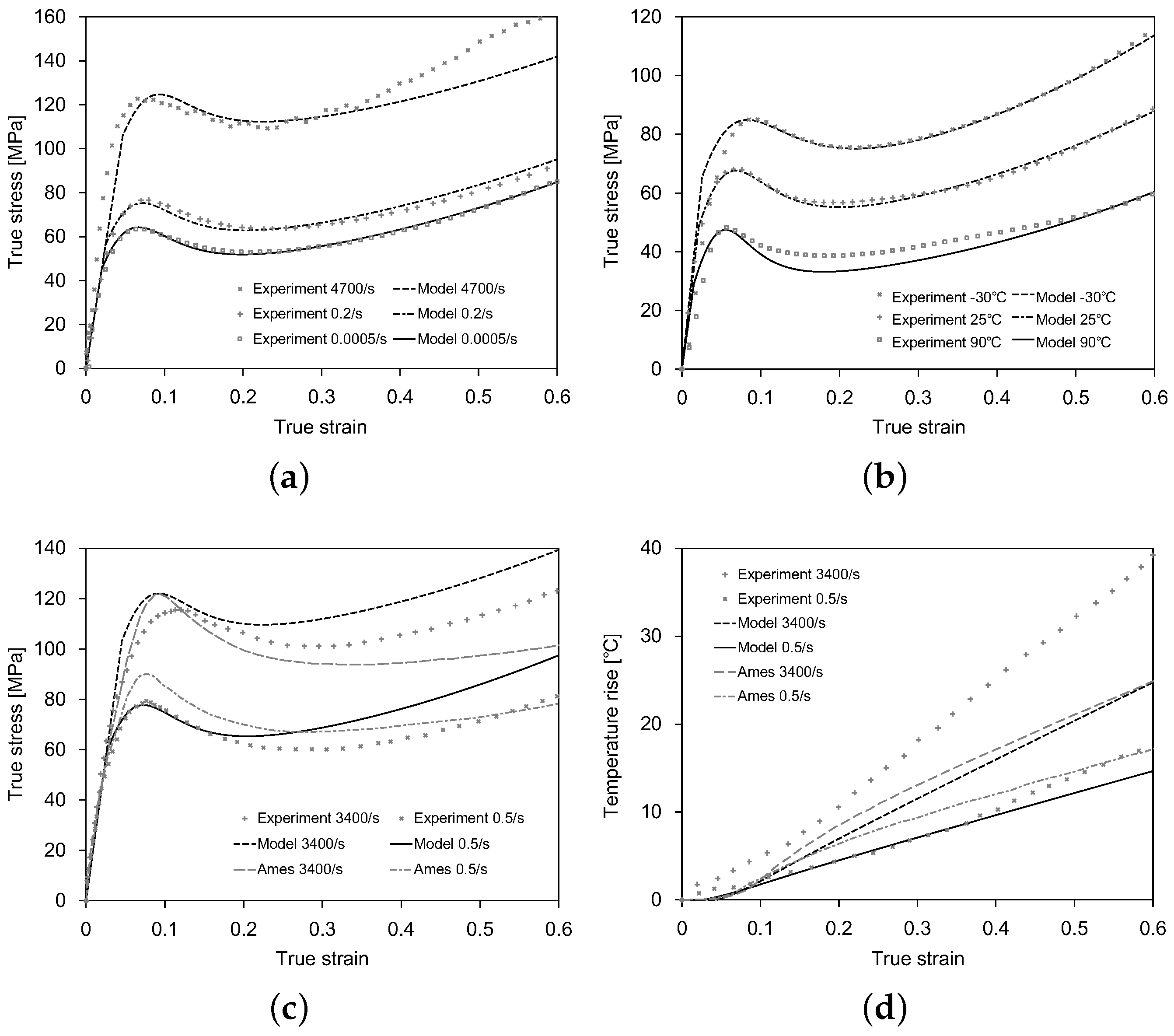
- The model parameters , , m, and control the dependence of the initial yield stress on the strain rate and temperature. The model parameter represents the initial yield stress at the minimum strain rate and the reference temperature , and it was determined approximately from the experimental stress-strain response at the strain rate of 0.0005 s−1 and the temperature of 25 °C. The model parameters and m were determined by fitting the exponential curve relationship between the yield stress and the logarithmic strain rate over the strain rate from 0.0005 s−1–8400 s−1. The model parameter was determined by fitting the linear relationship between the yield stress and the temperature over the temperature from −60 °C–120 °C. See the literature [25] for more details.
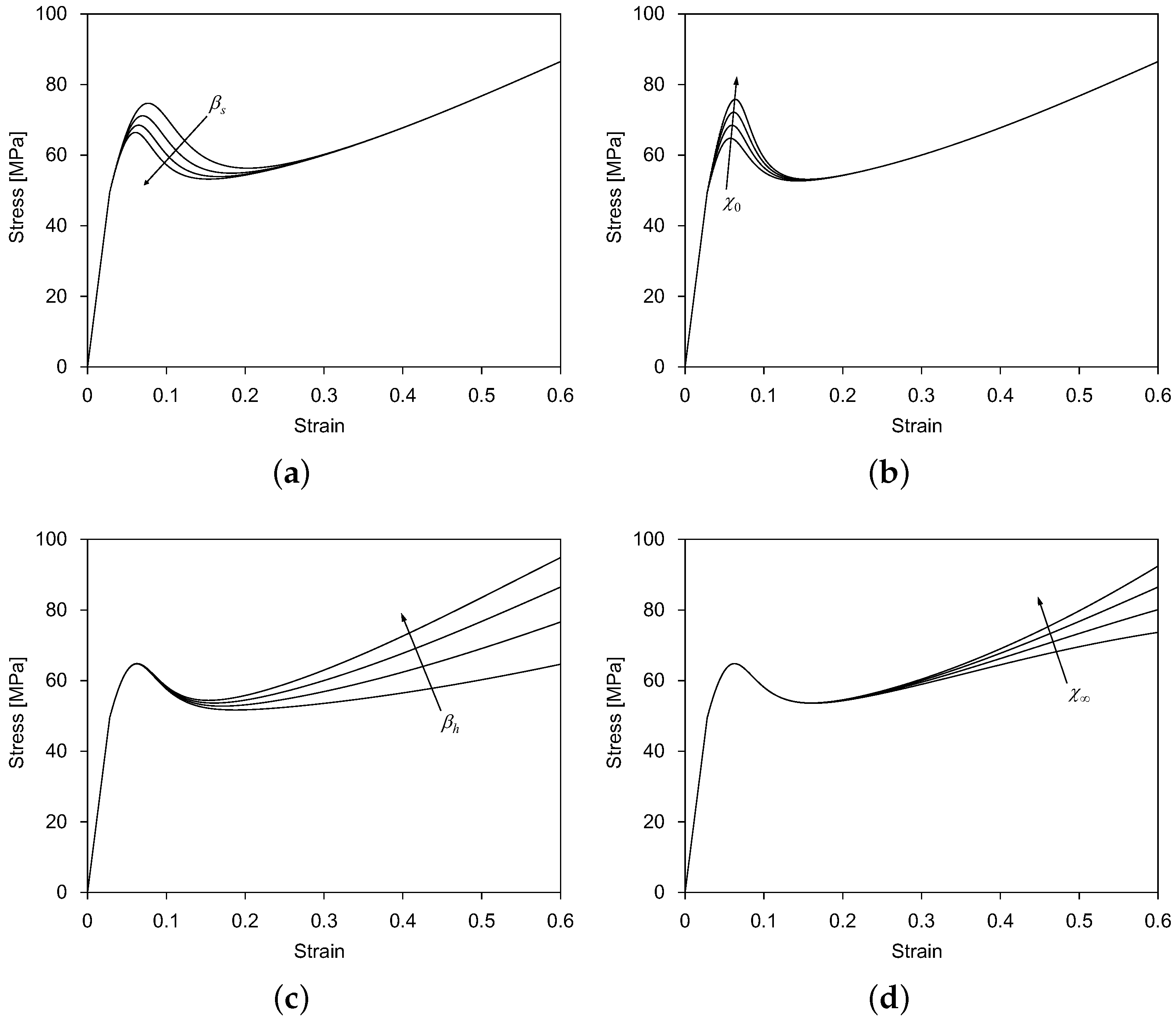
- The strain softening-associated model parameters , , , , and control the evolution of the internal variable . According to Equation (9), and are used to compute the state variable , while and are used to compute the state variable . Figure 1a,b shows how the parameters and affect the strain softening behavior of amorphous polymers. , , and were determined from the experimental stress-strain response at the reference temperature , while and were determined from the experimental stress-strain response at different temperatures.
- The strain hardening-associated model parameters , , , , and control the evolution of the internal variable . According to Equation (11), and are used to compute the state variable , while and are used to compute the state variable . Figure 1c,d shows how the parameters and affect the strain hardening behavior of amorphous polymers. , , and are determined from the experimental stress-strain response at the reference temperature , while and are determined from the experimental stress-strain response at different temperatures.
- The specific heat capacity c, the thermal conductivity k, and the mass density were obtained from the literature [26]. The Taylor–Quinney factor was determined from the temperature change experimentally measured by the thermal imager. The reference temperature took the room temperature of 25 °C.
3.3. Model Validation
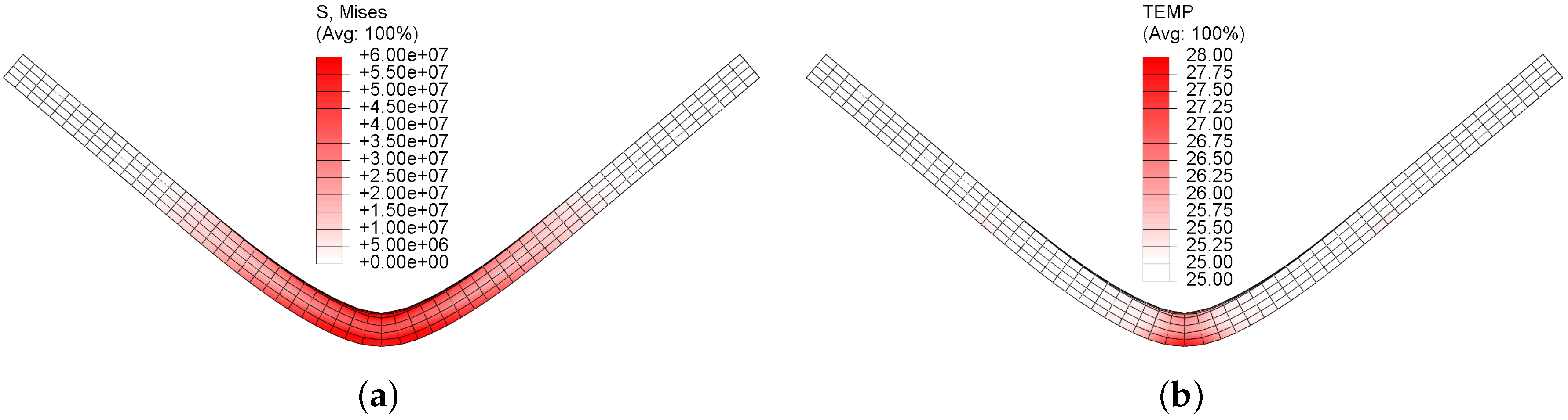
4. Three-Point Bending
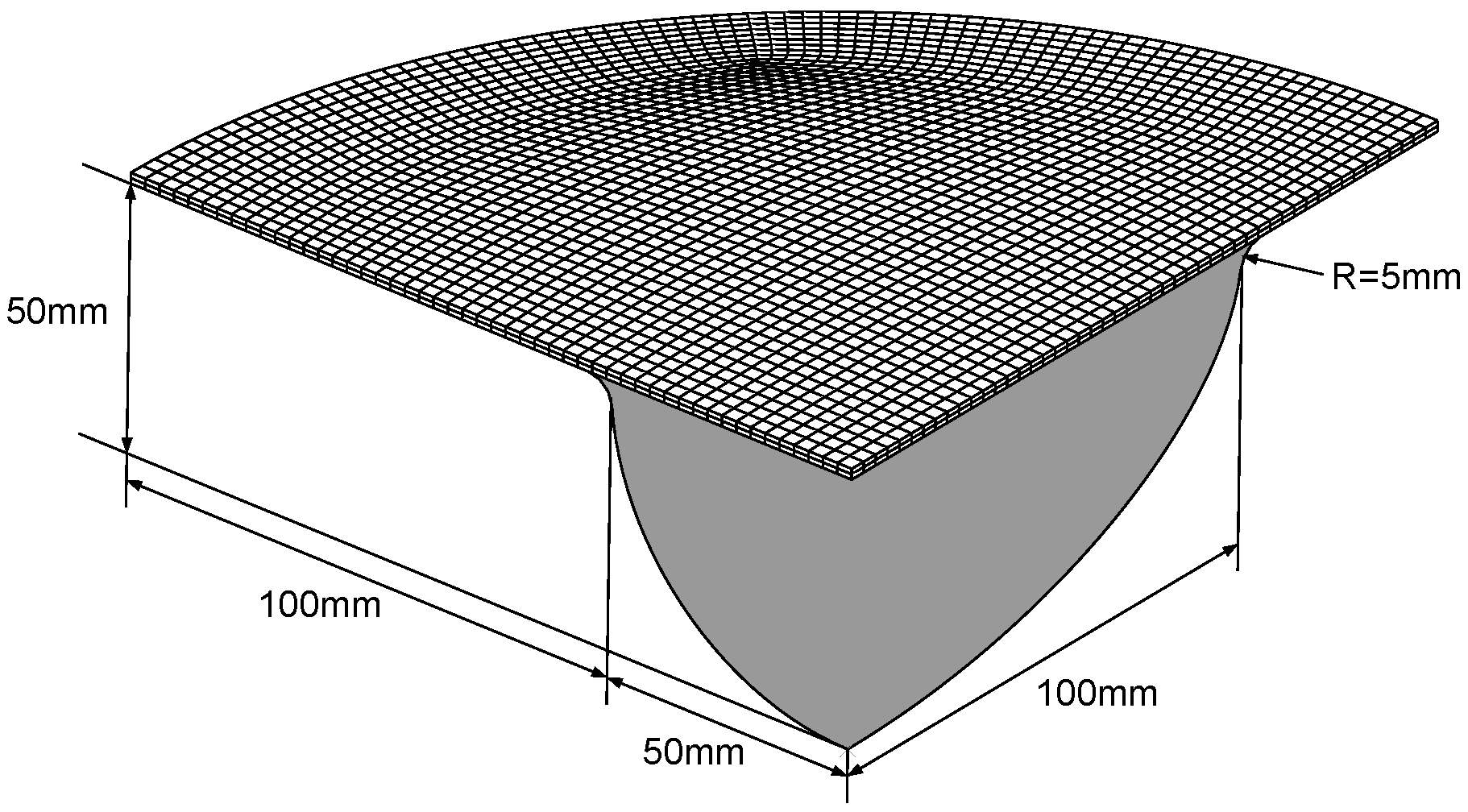
5. Gas-Blow Forming
6. Conclusions
Author Contributions
Acknowledgments
Conflicts of Interest
References
- Wang, J.; Xu, Y.; Zhang, W. Finite element simulation of PMMA aircraft windshield against bird strike by using a rate and temperature dependent nonlinear viscoelastic constitutive model. Compos. Struct. 2014, 108, 21–30. [Google Scholar] [CrossRef]
- Xu, Y.; Gao, T.; Wang, J.; Zhang, W. Experimentation and Modeling of the Tension Behavior of Polycarbonate at High Strain Rates. Polymers 2016, 8, 63. [Google Scholar] [CrossRef]
- Boyce, M.C.; Parks, D.M.; Argon, A.S. Large inelastic deformation of glassy polymers. Part I: Rate dependent constitutive model. Mech. Mater. 1988, 7, 15–33. [Google Scholar] [CrossRef]
- Ames, N.M.; Srivastava, V.; Chester, S.A.; Anand, L. A thermo-mechanically coupled theory for large deformations of amorphous polymers. Part II: Applications. Int. J. Plast. 2009, 25, 1495–1539. [Google Scholar] [CrossRef]
- Xu, Y.; Zhang, Q.W.; Zhang, W.; Zhang, P. Optimization of injection molding process parameters to improve the mechanical performance of polymer product against impact. Int. J. Adv. Manuf. Technol. 2015, 76, 2199–2208. [Google Scholar] [CrossRef]
- Yu, P.; Yao, X.; Han, Q.; Zang, S.; Gu, Y. A visco-elastoplastic constitutive model for large deformation response of polycarbonate over a wide range of strain rates and temperatures. Polymer 2014, 55, 6577–6593. [Google Scholar] [CrossRef]
- Achour, N.; Chatzigeorgiou, G.; Meraghni, F.; Chemisky, Y.; Fitoussi, J. Implicit implementation and consistent tangent modulus of a viscoplastic model for polymers. Int. J. Mech. Sci. 2015, 103, 297–305. [Google Scholar] [CrossRef]
- Mirkhalaf, S.M.; Andrade Pires, F.M.; Simoes, R. Modelling of the post yield response of amorphous polymers under different stress states. Int. J. Plast. 2017, 88. [Google Scholar] [CrossRef]
- Mei, Y.; Stover, B.; Kazerooni, N.A.; Srinivasa, A.; Hajhashemkhani, M.; Hematiyan, M.R.; Goenezen, S. A comparative study of two constitutive models within an inverse approach to determine the spatial stiffness distribution in soft materials. Int. J. Mech. Sci. 2018, 140, 446–454. [Google Scholar] [CrossRef]
- Boyce, M.C.; Arruda, E.M.; Jayachandran, R. The large strain compression, tension, and simple shear of polycarbonate. Polym. Eng. Sci. 1994, 34, 716–725. [Google Scholar] [CrossRef]
- Danielsson, M.; Parks, D.M.; Boyce, M.C. Micromechanics, macromechanics and constitutive modeling of the elasto-viscoplastic deformation of rubber-toughened glassy polymers. J. Mech. Phys. Solids 2007, 55, 533–561. [Google Scholar] [CrossRef]
- Buckley, C.P.; Jones, D.C. Glass-rubber constitutive model for amorphous polymers near the glass transition. Polymer 1995, 36, 3301–3312. [Google Scholar] [CrossRef]
- Wu, J.J.; Buckley, C.P. Plastic deformation of glassy polystyrene: A unified model of yield and the role of chain length. J. Polym. Sci. Part B Polym. Phys. 2004, 42, 2027–2040. [Google Scholar] [CrossRef]
- Li, H.X.; Buckley, C.P. Necking in glassy polymers: Effects of intrinsic anisotropy and structural evolution kinetics in their viscoplastic flow. Int. J. Plast. 2010, 26, 1726–1745. [Google Scholar] [CrossRef]
- Tervoort, T.A.; Govaert, L.E. Strain-hardening behavior of polycarbonate in the glassy state. J. Rheol. 2000, 44, 1263–1277. [Google Scholar] [CrossRef]
- Govaert, L.E.; Tervoort, T.A. Strain hardening of polycarbonate in the glassy state: Influence of temperature and molecular weight. J. Polym. Sci. Part B Polym. Phys. 2004, 42, 2041–2049. [Google Scholar] [CrossRef]
- Poluektov, M.; Van Dommelen, J.A.W.; Govaert, L.E.; Geers, M.G.D. Micromechanical modelling of reversible and irreversible thermo-mechanical deformation of oriented polyethylene terephthalate. Comput. Mater. Sci. 2015, 98, 189–200. [Google Scholar] [CrossRef]
- Anand, L.; Ames, N.M.; Srivastava, V.; Chester, S.A. A thermo-mechanically coupled theory for large deformations of amorphous polymers. Part I: Formulation. Int. J. Plast. 2009, 25, 1474–1494. [Google Scholar] [CrossRef]
- Bouvard, J.; Ward, D.; Hossain, D.; Nouranian, S.; Marin, E.; Horstemeyer, M. Review of Hierarchical Multiscale Modeling to Describe the Mechanical Behavior of Amorphous Polymers. J. Eng. Mater. Technol. 2009, 131, 041206. [Google Scholar] [CrossRef]
- Bouvard, J.L.; Ward, D.K.; Hossain, D.; Marin, E.B.; Bammann, D.J.; Horstemeyer, M.F. A general inelastic internal state variable model for amorphous glassy polymers. Acta Mech. 2010, 213, 71–96. [Google Scholar] [CrossRef]
- Bouvard, J.L.; Francis, D.K.; Tschopp, M.A.; Marin, E.B.; Bammann, D.J.; Horstemeyer, M.F. An internal state variable material model for predicting the time, thermomechanical, and stress state dependence of amorphous glassy polymers under large deformation. Int. J. Plast. 2013, 42, 168–193. [Google Scholar] [CrossRef]
- Fleischhauer, R.; Dal, H.; Kaliske, M.; Schneider, K. A constitutive model for finite deformation of amorphous polymers. Int. J. Mech. Sci. 2012, 65, 48–63. [Google Scholar] [CrossRef]
- Nada, H.; Hara, H.; Tadano, Y.; Shizawa, K. Molecular chain plasticity model similar to crystal plasticity theory based on change in local free volume and FE simulation of glassy polymer. Int. J. Mech. Sci. 2015, 93, 120–135. [Google Scholar] [CrossRef]
- Bai, Y.; Liu, C.; Huang, G.; Li, W.; Feng, S. A hyper-viscoelastic constitutive model for polyurea under uniaxial compressive loading. Polymers 2016, 8, 133. [Google Scholar] [CrossRef]
- Wang, J.; Xu, Y.; Zhang, W.; Moumni, Z. A damage-based elastic-viscoplastic constitutive model for amorphous glassy polycarbonate polymers. Mater. Des. 2016, 97, 519–531. [Google Scholar] [CrossRef]
- Wang, J.; Xu, Y.; Gao, T.; Zhang, W.; Moumni, Z. A 3D thermomechanical constitutive model for polycarbonate and its application in ballistic simulation. Polym. Eng. Sci. 2018, 58, 2237–2248. [Google Scholar] [CrossRef]
- Xiao, H.; Bruhns, O.; Meyers, A. Explicit dual stress-strain and strain-stress relations of incompressible isotropic hyperelastic solids via deviatoric Hencky strain and Cauchy stress. Acta Mech. 2004, 168, 21–33. [Google Scholar] [CrossRef]
- Reinhardt, W.D.; Dubey, R.N. Application of objective rates in mechanical modeling of solids. J. Appl. Mech. 1996, 63, 692–698. [Google Scholar] [CrossRef]
- Wang, J.; Moumni, Z.; Zhang, W.; Xu, Y.; Zaki, W. A 3D finite-strain-based constitutive model for shape memory alloys accounting for thermomechanical coupling and martensite reorientation. Smart Mater. Struct. 2017, 26. [Google Scholar] [CrossRef]
- Dafalias, Y.F. The plastic spin concept and a simple illustration of its role in finite plastic transformations. Mech. Mater. 1984, 3, 361. [Google Scholar] [CrossRef]
- Wang, J.; Xu, Y.; Zhang, W.; Wang, W. A finite-strain thermomechanical model for severe superplastic deformation of Ti-6Al-4V at elevated temperature. J. Alloys Compd. 2019, 787, 1336–1344. [Google Scholar] [CrossRef]
- Wang, J.; Moumni, Z.; Zhang, W.; Zaki, W. A thermomechanically coupled finite deformation constitutive model for shape memory alloys based on Hencky strain. Int. J. Eng. Sci. 2017, 117, 51–77. [Google Scholar] [CrossRef]
- Mahieux, C.A.; Reifsnider, K.L. Property modeling across transition temperatures in polymers: A robust stiffness—Temperature model. Polymer 2001, 42, 3281–3291. [Google Scholar] [CrossRef]
- Wang, J.; Moumni, Z.; Zhang, W. A thermomechanically coupled finite-strain constitutive model for cyclic pseudoelasticity of polycrystalline shape memory alloys. Int. J. Plast. 2017, 97, 194–221. [Google Scholar] [CrossRef]
- Garg, M.; Mulliken, A.D.; Boyce, M.C. Temperature rise in polymeric materials during high rate deformation. J. Appl. Mech. 2008, 75, 11009. [Google Scholar] [CrossRef]


| Elasticity: , , , ; |
| Yielding: , , m, ; |
| Softening: , , , , ; |
| Hardening: , , , , ; |
| Heat: c, k, , , . |
| Categories | Parameters | Constants | Values |
|---|---|---|---|
| Elasticity | E (MPa) | (MPa) | 2271 |
| (MPa/K) | −5.4 | ||
| 0.4 | |||
| (K−1) | |||
| Yielding | (MPa) | 35.16 | |
| (s) | 0.746 | ||
| m | 0.118 | ||
| (K−1) | |||
| Softening () | (MPa) | 130.45 | |
| 0.036 | |||
| (K−1) | 10.24 | ||
| 0.105 | |||
| (K−1) | 26.86 | ||
| Hardening () | (MPa) | 82.36 | |
| −0.012 | |||
| (K−1) | 3.12 | ||
| 1.45 | |||
| (K−1) | 6.46 | ||
| Heat | c (J/(kg · K)) | ||
| k (W/(m · K)) | 0.19 | ||
| (kg/m3) | |||
| 0.86 | |||
| (K) | 298 |
| Gas Pressure | Major Axis | Minor Axis |
|---|---|---|
| Pressurization 1.0 MPa |  |  |
| Pressurization 2.0 MPa | 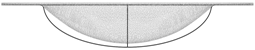 | 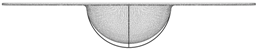 |
| Pressurization 3.0 MPa |  | 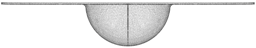 |
| Depressurization 0.0 MPa | 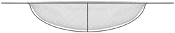 |  |
© 2019 by the authors. Licensee MDPI, Basel, Switzerland. This article is an open access article distributed under the terms and conditions of the Creative Commons Attribution (CC BY) license (http://creativecommons.org/licenses/by/4.0/).
Share and Cite
Wang, J.; Xu, Y.; Zhang, W.; Ren, X. Thermomechanical Modeling of Amorphous Glassy Polymer Undergoing Large Viscoplastic Deformation: 3-Points Bending and Gas-Blow Forming. Polymers 2019, 11, 654. https://doi.org/10.3390/polym11040654
Wang J, Xu Y, Zhang W, Ren X. Thermomechanical Modeling of Amorphous Glassy Polymer Undergoing Large Viscoplastic Deformation: 3-Points Bending and Gas-Blow Forming. Polymers. 2019; 11(4):654. https://doi.org/10.3390/polym11040654
Chicago/Turabian StyleWang, Jun, Yingjie Xu, Weihong Zhang, and Xuanchang Ren. 2019. "Thermomechanical Modeling of Amorphous Glassy Polymer Undergoing Large Viscoplastic Deformation: 3-Points Bending and Gas-Blow Forming" Polymers 11, no. 4: 654. https://doi.org/10.3390/polym11040654
APA StyleWang, J., Xu, Y., Zhang, W., & Ren, X. (2019). Thermomechanical Modeling of Amorphous Glassy Polymer Undergoing Large Viscoplastic Deformation: 3-Points Bending and Gas-Blow Forming. Polymers, 11(4), 654. https://doi.org/10.3390/polym11040654