Lateral Diffusion of a Free Air Jet in Slot-Die Melt Blowing for Microfiber Whipping

Abstract

In melt blowing, microfibrous nonwoven material is manufactured by using high-speed air to attenuate polymer melt. The melt-blown air jet determines the process of polymer attenuation and fiber formation. In this work, the importance of lateral velocity on the fiber was first theoretical verified. The lateral diffused characteristic of the air flow field in slot-die melt blowing was researched by measuring the velocity direction using a dual-wire probe hot-wire anemometer. Meanwhile, the fiber path was captured by high-speed photography. Results showed that there existed a critical boundary of the lateral diffusion, however, air jets in the x–z plane are a completely diffused field. This work indicates that the lateral velocity in the y–z plane is one of the crucial factors for initiating fiber whipping and fiber distribution.

1. Introduction

Melt blowing is an industrial approach for manufacturing nonwoven materials. Melt-blown nonwoven materials have found a variety of advanced applications in areas of filtration, life science, medicine, and industry [1,2], the fiber diameter is commonly in the range from about 1 μm to several micrometers.

During the melt blowing process, the raw material of solid particles is melted by the effects of heating and the screw’s shear stress, and subsequently extruded out through the orifice, the microfibers are formed by attenuating the melt with high-velocity hot air (see Figure 1). Therefore, the air flow field plays a decisive role on fiber attenuation (formation) during melt blowing. Shambaugh et al. [3,4,5,6] have relatively early measured the air velocity and temperature by Pitot tube and thermocouples (or infrared thermometer), respectively, in the condition of relatively low air velocity. Later, more-advanced measuring equipment like laser Doppler velocimeters and hot-wire anemometers with one-dimensional probes were applied for measuring the melt-blown air flow fields [7,8,9,10,11], the maximum air velocity they measured increased to be about 150 m/s. By means of the high-frequency signal acquisition principle of the hot-wire anemometer, Xie [11] measured the fluctuation of turbulence in melt blowing and discussed the relationship between turbulence and fiber motion. It noted that, air velocity is a vector and has the characteristics of directivity, however, these previous experimental measurements provided the velocity along the spinning line, the directional information of velocity was unavailable, especially for positions not along the spinning line, generally, these measured velocities were considered to have a direction parallel to the spinning line. Therefore, the air flow field was researched with a lack of information along the lateral direction.

In melt blowing, the air is pushed out from air channels and ejected into the surrounding static atmospheric, therefore, the melt-blown air flow needs to be a free jet and have the feature of diffusion, that is, the cross-section of the air flow is ever increasing along the spinning line direction. The diffusion of air flow could be demonstrated by a lot of Computational Fluid Dynamics (CFD) simulations [9,12] and indirectly reflected by the splayed-out envelope of the fiber path, which is attributed to fiber vibration or whipping in the process of melt blowing [13,14,15]. A bundle of fibers that appeared to be splaying rather than a single fiber was firstly captured by Shambaugh [13]. This observation was similar to that from the naked eye. Similar splayed-out envelopes of fiber paths were also experimentally discovered by Bresee et al. [14] and Xie [15]. The increased envelope of the fiber path is assumed by the lateral air velocity component (direction normal to the spinning line), however, until now, the measurement of the lateral velocity component has not been reported and most of the air flow fields were measured along the spinning-line direction.

In addition, the theoretical research on fiber motion is important, for it can deeply reveal the stretching mechanism of fiber attenuation in the spinning process, not only for melt blowing but also for other process such as electrospinning [16]. The theory of the bending instability of thin liquid jets in air was developed and described by Yarin [17]. Rao [18] and Marla [19] built two- and three-dimensional theoretical models for fiber attenuation in melt blowing, respectively. Compared to the former one-dimensional model [20], the normal drag force was applied onto the fiber. Bates, Kumar, and Macosko from the University of Minnesota [21,22,23,24,25,26,27] have done some theoretical and experimental work on fiber formation, special applications, and innovative designing of melt blowing. Kumar [23] firstly point out that, in melt blowing, the whipping-like motion of the fiber was due to turbulent air, this guidance promoted our previous work on the turbulence of melt blowing [11,15]. Yarin et al. [28,29,30,31,32] have numerical modeled the process of fiber motion and predicted the structure and properties of melt-blown nonwoven lay-down. Their works are assumed to have a crucial effect on quality control in melt blowing. Sun [33] built a Euler–Lagrange model for the mechanics simulation of fiber motion during the melt-blown process, and this model was improved to make the fiber path more realistic by Xie et al. [34] These theoretical models focused on mechanical mechanisms, rather than citing detailed air information of the whole air flow field. Therefore, the discovery of more consummate flow field information will contribute to perfecting these theoretical researches.

It is well known that the melt-blown air’s resultant velocity can be decomposed into vertical and lateral components, i.e., their directions are parallel and normal to the spinning line, respectively. The present work focused on discovering the lateral component of the air flow in slot-die melt blowing. Firstly, the significance or necessity of measuring the lateral velocity was theoretical verified. The theoretical result showed that the lateral component had high efficiency on fiber dragging, and should not be ignored. Then, the air velocity direction was measured by a dual-wire hot-wire anemometer, and the lateral air velocity component was obtained by processing the measured velocity direction, meanwhile, the fiber path during melt blowing was captured by high-speed photography. Finally, the characteristics of lateral diffusion were shown, and the potential effect of lateral diffusion on fiber whipping was discussed.

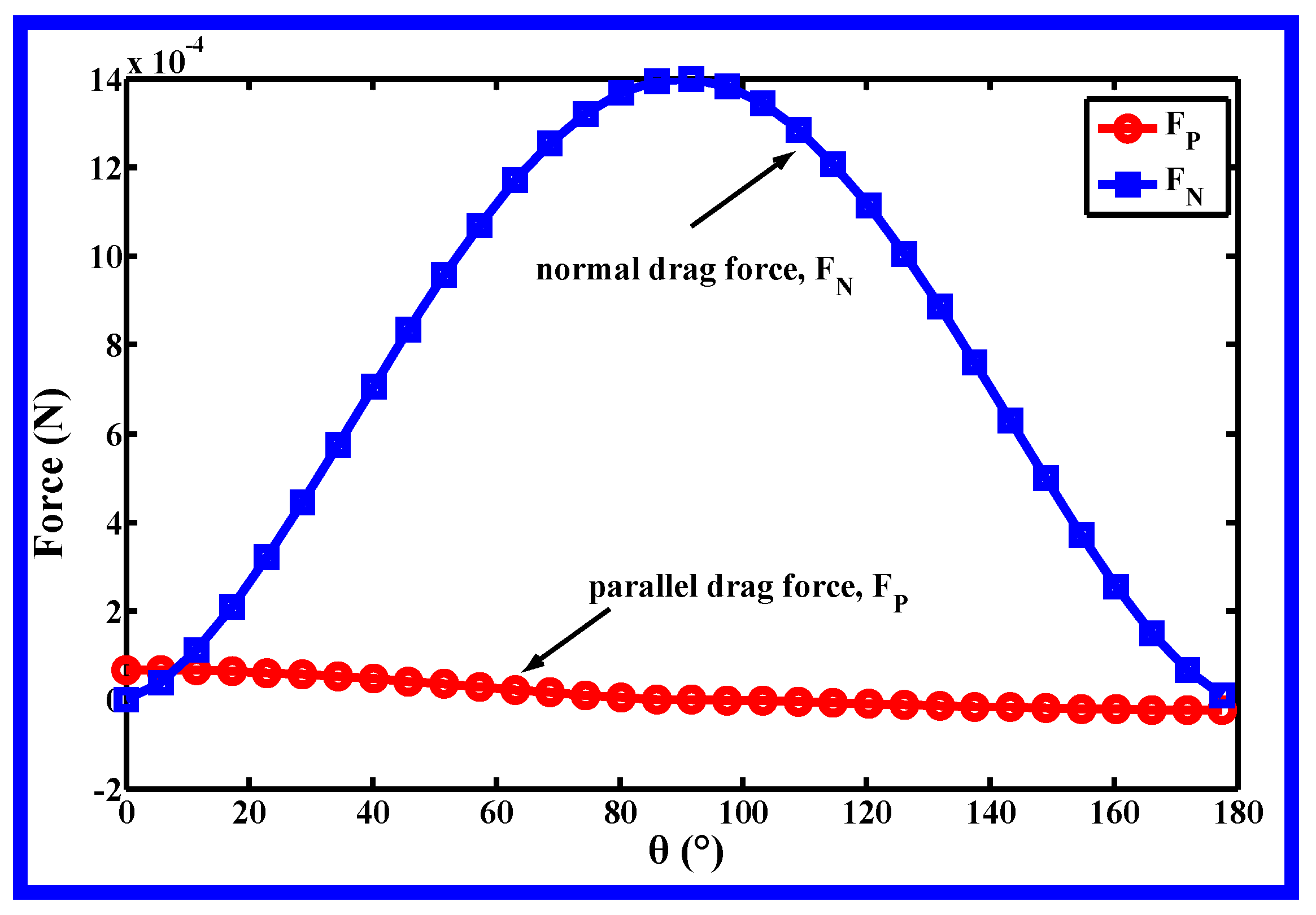
2. Theoretical Verification the Importance of Lateral Velocity

Figure 1a shows the schematic process of melt blowing, in which microfibers are manufactured by attenuating the polymeric melt with high-velocity hot air. As a whole, the fibers will fly along the spinning line and downward to the collector. Figure 1b shows the microfiber nonwovens manufactured by melt blowing. In this work, the spinning line is the indicated z-axis, and the lateral direction is normal to the spinning line, i.e., along the x or y direction.

Intuitively, the lateral air component is very small, this may be the reason why the lateral component was neglected by these previous works, which have been mentioned above. As will be described below, the importance or necessity of lateral component measurement was firstly verified by theoretical force analysis.

This theoretical verification was carried out by analyzing the air force on the fiber. As shown in Figure 1c, a random tiny fragment of fiber was chosen for modeling. During the process of melt blowing, it was assumed that the fiber fragment has a two-dimensional resultant velocity, v_f, which can decomposed into parallel and normal components with respect to the axis-direction of the fiber, i.e., v_fP and v_fN. Similarly, the air applied on the fiber fragment has a resultant velocity, v_r, by decomposing v_r into parallel and normal components with respect to axis-direction of the fiber, v_P and v_N are obtained. The angle between v_r and the axis of the fiber is θ. The relative velocity of the air and the fiber, v_rel, can decompose into

$$v_{rel,P}=v_r\cos (\theta )-v_{fP}(0\le \theta \le {180}^{°}),$$

(1a)

$$v_{rel,N}=v_r\sin (\theta )-v_{fN}(0\le \theta \le {180}^{°}),$$

(1b)

where v_rel,P and v_rel,N are the component velocities of the relative velocity, which are parallel and normal to the axis of the fiber.

Components velocities of v_rel,P and v_rel,N, respectively, create accordingly a “parallel drag force”, F_P, and a “normal drag force”, F_N, on the fiber [18]. The appropriate definitions for the two drag forces are

$$F_P=\frac{1}{2}{C}_P{\rho }_a{(v_{rel,P})}^2(\pi d_f{l}_f),$$

(2a)

$$F_N=\frac{1}{2}{C}_N{\rho }_a{(v_{rel,N})}^2(d_f{l}_f),$$

(2b)

where C_P and C_N are the skin coefficient and the drag coefficient, respectively; ρ_a is the density of air; and d_f and l_f represent the diameter and length of the fiber fragment, respectively. Additionally, there are also the following relationships [35,36,37].

$$C_P=0.78{({\mathrm{Re}}_{DP})}^{-0.61},$$

(3a)

$$C_N=6.96{({\mathrm{Re}}_{DN})}^{-0.440}{(d_f/d_0)}^{0.404},$$

(3b)

$${\mathrm{Re}}_{DP}=\frac{{\rho }_a{v}_{rel,P}{d}_f}{{\mu }_a},$$

(4a)

$${\mathrm{Re}}_{DN}=\frac{{\rho }_a{v}_{rel,N}{d}_f}{{\mu }_a},$$

(4b)

where μ_a is the kinematic viscose of air; d₀ is 7.8 × 10⁻⁵ m [37].

Substituting Equations (3a) and (4a) into Equation (2a), and substituting Equations (3b) and (4b) into Equation (2b), F_P and F_N are

$$F_P=0.39\pi \frac{{{\rho }_a}^{0.39}{(v_r\cos (\theta )-v_{fP})}^{1.39}{d_f}^{0.39}{l}_f}{{({\mu }_a)}^{-0.61}}$$

(5a)

$$F_N=159\frac{{{\rho }_a}^{0.56}{(v_r\sin (\theta )-v_{fN})}^{1.56}{d_f}^{0.964}{l}_f}{{{\mu }_a}^{-0.440}}.$$

(5b)

Because the fiber velocity is much smaller than the air velocity [15], here, v_f is simplified to be 0 m/s, i.e., v_fP and v_fN are all zero. Substituting ρ_a =1.293 kg/m³, μ_a = 0.297 × 10⁻⁴ Pa·s, and assuming d_f = 0.42 × 10⁻³ m, l_f = 10⁻³ m, and v_r = 100 m/s in Equation (5), the relationships between F_P, F_N, and θ are

$$F_P=6.81\times {10}^{-5}{\cos }^{1.39}(\theta )(0\le \theta \le {180}^{°})$$

(6a)

$$F_N=1.40\times {10}^{-3}{\sin }^{1.56}(\theta )(0\le \theta \le {180}^{°}).$$

(6b)

Figure 2 shows F_P, F_N with respect to θ under the same assumption. The F_N is much higher than the F_P at the same θ, especially when θ is around 90°. The force analysis of the fiber illustrates that even if the lateral velocities, v_x and v_y, are not as large as the spinning-line-direction velocity component, v_z [11], lateral velocities have higher efficiency on dragging fibers. Additionally, the force analysis shows the measurement of lateral diffusion is meaningful.

3. Experiments

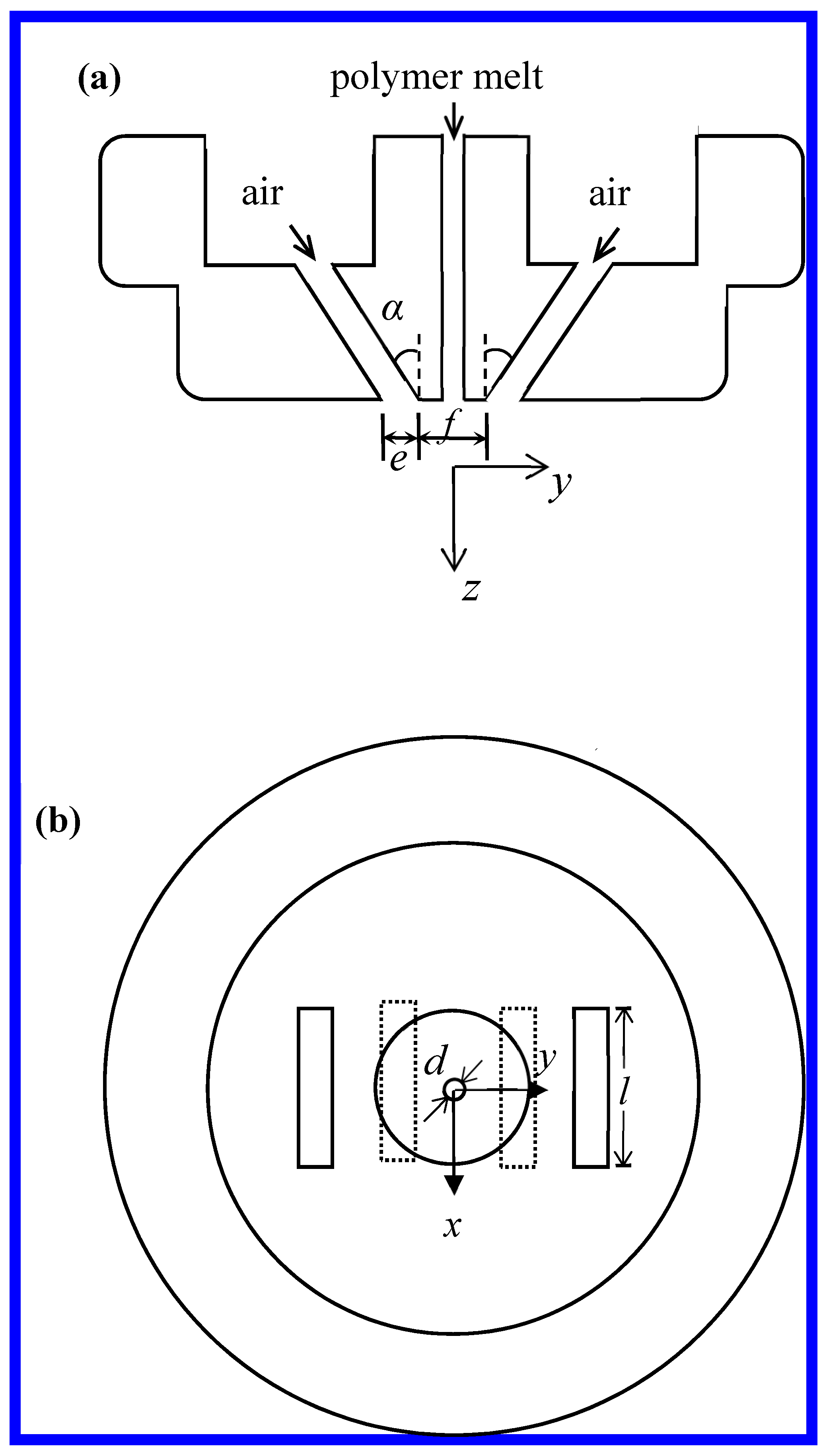
3.1. Melt-Blown Setups

The measurement of air velocity direction in this study was performed on the single-orifice slot-die melt-blown device (if the multifibers, shown in Figure 1a, are changed to be single fiber, then the single-orifice slot-die melt-blown process is shown). The structure of the slot die used in this work is shown in Figure 3. Slot die is referred to as a blunt-edge with a nose-piece width (f) of 1.28 mm, a slot angle (α) of 30°, and a slot width (e) of 0.65 mm, the orifice diameter for the polymer melt (d) was 0.42 mm. Other details of this slot die can be found in the manuscript of Xie [15], this kind of die was also described by other researchers [3,10]. The coordinate system used is also shown in Figure 3, all coordinates are relative to the die face. Its origin is at the center of the die face, the x direction is along the major axis of the nose piece and slots, whereas the y direction is transverse to the major axis of the nose piece and slots. The z direction is directed vertically downward.

3.2. Air Velocity Direction Measurements

As shown in Figure 4a, the velocity direction below the die was online measured with a hot-wire anemometer (Dantec StreamLine CTA90C10, Dantec Dynamics, Skovlunde, Denmark) in the absence of the polymer stream. A gauge air pressure of 1.0 atm was supplied for measurement. This anemometer is often called CTA or constant temperature anemometer with reference to the operating principle. The CTA works on the basis of convective heat transfer from a hot wire to the surrounding fluid, the heat transfer being primarily related to the fluid velocity, namely, the melt-blowing air takes away the heat of the wire, the temperature of the wire is kept constant by applying voltage on it. The relationship between air velocity and the applied voltage is

$$\frac{E}{R_w}=[\frac{(R_w-R_f)(A+B{v}^{1/2})}{{\alpha }_0{R}_f{R}_w}],$$

(7)

where E is the heating voltage applied on the wire; R_w and R_f are the resistance of the wire at temperature of wire and air, respectively; A and B are constant numbers; v is the air velocity; and α₀ is the temperature coefficient of resistance.

The CTA signal was acquired via an A/D converter board and saved as a data series in a computer. Series of air velocities were obtained by converting the data series of voltages via Equation (7). Actually, the so-called air velocity refers to the mean of the data series of velocities. As a core component of the CTA, probes are available in one-, two-, and three-dimensional versions as single-, dual-, and triple-wire probes referring to the number of wires. Since the wires respond to both magnitude and direction of the velocity vector, information about both can be obtained, only when two or more wires are placed under different angles to the flow vector. A dual-wire probe was attempted for the velocity-direction measurement in this work, Figure 4b illustrates the structure of the dual-wire probe used in this measurement, the dual-wire probe consisted of two systems of single-wire probes, each probe had a wire with a 5 μm diameter and a 1.6 mm length spot-welded to needle-shaped prongs, made of stainless steel. The two planes which contain the two wires and their corresponding prongs were parallel to each other, the projections on the parallel planes of the two wires were vertical. Note that the arrangement of the two wires was very important during measurement, for example, the plane which contains the two wires and its corresponding prongs is in the x–z plane, with this arrangement, the angle between the projection of the air velocity in the x–z plane and the z-axis is measured. In the present work, the projection of the air velocity in the x–z plane was called velocity in x–z plane for short.

During the measurements of air velocity direction, the probe was positioned with a traversing system, which permitted upward or downward motion along the z-axis in 2 mm increments. In consideration of probe protection, the minimum distance below the die was set to z = 6 mm. The measurement was carried out on 384 discrete positions, these discrete positions were along eight series lines, they were

Positions along line 1: [x = 0, y = 2, z = 6, 8, 10, … 100 mm]

Positions along line 2: [x = 0, y = 5, z = 6, 8, 10, … 100 mm]

Positions along line 3: [x = 0, y = 10, z = 6, 8, 10, … 100 mm]

Positions along line 4: [x = 0, y = 20, z = 6, 8, 10, … 100 mm]

Positions along line 5: [x = 2, y = 0, z = 6, 8, 10, … 100 mm]

Positions along line 6: [x = 5, y = 0, z = 6, 8, 10, … 100 mm]

Positions along line 7: [x = 10, y = 0, z = 6, 8, 10, … 100 mm]

Positions along line 8: [x = 20, y = 0, z = 6, 8, 10, … 100 mm]

Calibration is an indispensable process before all formal measurements, similarly, before the air velocity direction measurement, the directional calibration was accomplished on a calibration device at ambient temperature. Calibration establishes a relationship between the CTA output and the air direction. As shown in Figure 5a, it was performed by exposing the probe to a known air velocity from different angles, two responding voltages (E₁ and E₂) could be obtained for the dual wires. By the principle of Equation (7), E₁ and E₂ were different, because of the angle of arrangement of the dual wires. Figure 5b shows the calibration angle and its two responding voltages for the dual wires, which is called the directional-calibration curve, the calibration angle, φ, was set from −40° to 40° with an interval of 10°. Here, the calibration angle and the ratio of E₁ and E₂ had a relationship of

$$\phi =\frac{1.0066-E_1/E_2}{0.0023}{\mathrm{R}}^2=0.9954.$$

(8)

Later, during the formal measurement, the air velocity direction could be calculated from the ratio of output of E₁ and E₂ according to Equation (8). In this measurement, the discovery of lateral diffusion was carried out by measuring the velocity direction in two typical vertical planes, i.e., y–z and x–z plane.

3.3. Fiber Path Measurement

Polypropylene (SK, Seoul, Korea) with melt flow rate of 650 g/10 min was used in the fiber spinning process. The base conditions were a polymer flow rate of 7.1 g/min, a polymer temperature of 260 °C, and a gauge air pressure of 1.0 atm with room temperature.

The melt-blown fiber motion was online captured by a high-speed camera (Redlake Inc., San Diego, CA, USA), which has the capability of recording images at a frame rate up to 100,000 partial frames/s. The camera was equipped with a Nikon 24–85 mm, f 2.8 zoom lens. Two 2000 W lamps were added as a light source to make the fiber more clear. Fiber paths in a region of 62.5 mm × 130 mm in the y–z plane and the x–z plane were captured, respectively, at the frame rate of 1500 frames/s. Similar measurements of the fiber path can be found in the previous work of Xie [15] or Shambaugh [38].

4. Results and Discussion

4.1. Air Velocity Direction

Figure 6 shows the directional angle between the z-axis and the resultant velocity in the y–z plane (here, resultant velocity in the y–z plane means the projection of the air resultant velocity on y–z plane), at different positions along lines 1–4 (lines 1–4 correspond to the lines of y = 2, 5, 10, and 20 mm in the y–z plane). The resultant velocity in the y–z plane consisted of the component velocities of v_y and v_z, where v_y was definitely the lateral component velocity.

Along line 1 of y = 2 mm, the angle down from the z-axis, φ, was about −8° at z = 6 mm, and increased to be a positive value at a critical position of z = 14 mm, the angle had a small increase in the distance beyond z = 14 mm, but all of them were less than 5°. Similarly, the angles along lines 2 and 3 of y = 5 and 10 mm, had minimum (negative) values at z = 6 mm, and increased with increasing distance from the die, at critical positions of z = 50 and 72 mm, the values of their angle changed to be positive. For the angle along line 4 of y = 20 mm, although the angle had a general increasing trend with increasing distance from the die, there existed a large angle fluctuation near the die, especially in the region of z < 40 mm, revealing that the velocity in the y–z plane became unstable in the lateral region far away from the spinning line, i.e., the z-axis. The reason for the instability was deduced to be caused by the collision of the air jet and the surrounding atmosphere. In Figure 6, the positive value represents that the direction of the resultant velocity deviates from the z-axis, i.e, v_y has a positive direction along the y-axis. Similarly, the negative value meant the v_y had opposite direction with the y-axis. According to this illustration, an interesting phenomenon can be discovered, namely that there exists a veer of lateral velocity in the slot-die melt-blown air flow field, which means that there exists a critical boundary of the lateral diffusion of air flow in the y–z plane during slot-die melt blowing.

Figure 7 shows the directional angle between the z-axis and the resultant velocity in the x–z plane, at different positions along lines 5–8 (lines 5–8 correspond to the positions of x = 2, 5, 10, and 20 mm in the x–z plane). The resultant velocity in the x–z plane consisted of component velocities of v_x and v_z, v_x is also the so-called lateral velocity in this work. Unlike the profiles of angles shown in Figure 6, all angles in Figure 7 are positive in value, indicating that the air jets in the x–z plane are a completely diffused field. Moreover, the angles commonly decrease with increasing distance from the die, implying that the lateral diffused effect decreases with increasing distance from the die.

Figure 8 shows the fluctuant signals of the angle between the resultant velocity in the y–z plane and the z-axis, at four lateral discrete positions, i.e., (y, z) = (2, 6), (5, 6), (10, 6), and (20 mm, 6 mm), respectively. A time segment of 2 s was chosen for the demonstration of the angle’s fluctuation. As shown in Figure 8, these fluctuant signals are irregular and different at different positions. These fluctuation signals were expected to contain lots of potential information, however, the investigation of the potential information of signals is not the topic of this work, therefore, the fluctuation signals at the other 380 positions (the total positions in this work is 384) are not shown in this part. Even so, it is certain that the polymeric fiber undergoes pulsating air force during melt blowing, which might be one reason for initiating fiber instability during melt blowing.

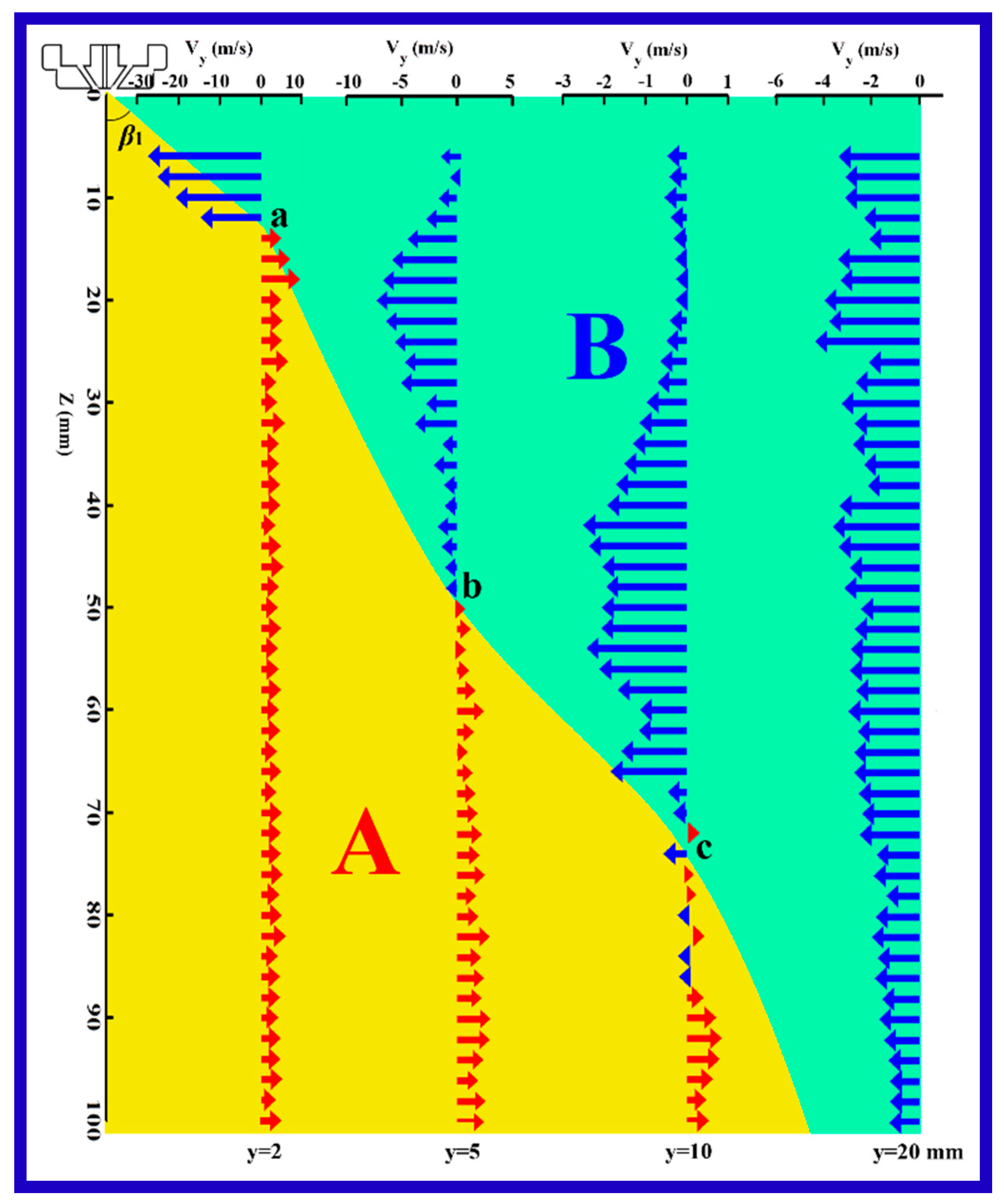
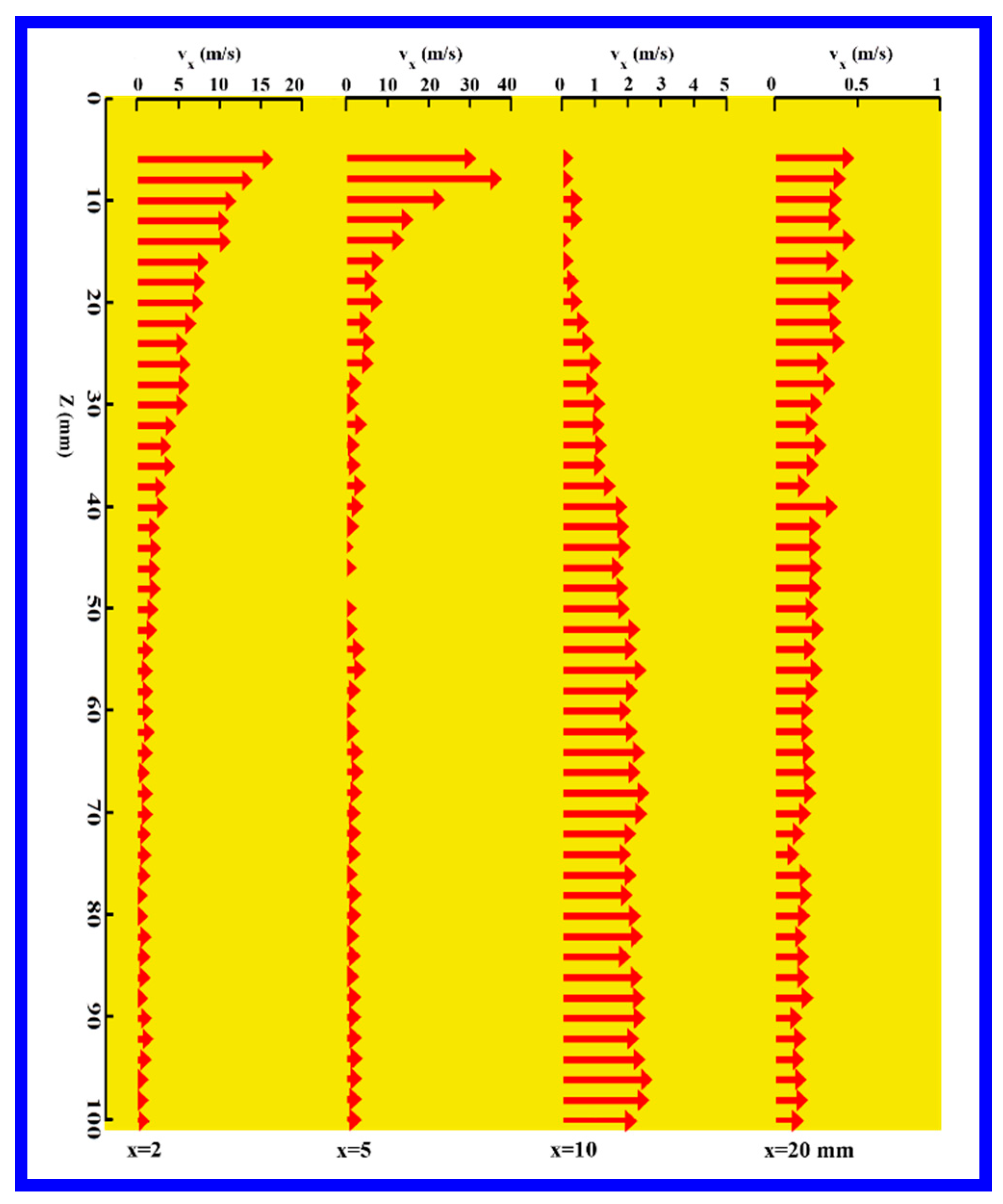
4.2. Lateral Velocity Components: v_y and v_x

Figure 9 shows the distribution of the lateral velocity, v_y, along lines 1–4 of y = 2, 5, 10, and 20 mm, in the corresponding y–z plane. Here, the lateral velocity component was calculated via multiplying resultant velocity by the angles, which are shown in Figure 6 and Figure 7. It should be pointed out that Figure 9 has a double abscissa, the upper and the lower abscissa are v_y and y positions, respectively. For the v_y along line 1 of y = 2 mm, the v_y had a magnitude of 28 mm/s and had back-diffusion direction within the positions above the point “a” signed in this figure, however, the v_y had a lateral diffused direction at positions below the critical point “a”. Here, ”a” is deemed to be the so-called boundary of veer, which has been mentioned above. At positions along lines 2 and 3 of y = 5 and 10 mm, v_y has similar profiles to v_y along line 1, moreover, the maximum value of v_y decreased laterally far away from the z-axis, and the boundary points of veer are signed “b” and “c”, respectively. However, for the v_y along line 4 of y = 20 mm, all v_y has back-diffusion direction, even though the maximum v_y is as small as about 4.5 m/s. In a word, as shown in Figure 9, air flow has the characteristic of lateral diffusion in region A (yellow region), and lateral back-diffusion in the region B (green region). To further represent the lateral diffused characteristic of air flow in the y–z plane, a diffused envelope angle, β, is built, which is defined by Equation (9) below. Furthermore, β is calculated to be about 17.1°.

$$\beta =2\left(\frac{{\beta }_1+{\beta }_2+{\beta }_3}{3}\right),$$

(9)

where β₁ is the angle between the z-axis and the line segment of origin and “a”; similarly, β₂ is the angle between the z-direction and the line segment of “a” and “b”, and β₃ is the angle between the z-direction and the line segment of “b” and “c”. Here, the y–z coordinates of “a”, “b”, and “c” are (2, 14), (5, 50), and (10 mm, 72 mm).

Figure 10 shows the distribution of lateral velocity, v_x, along lines 5–8 of x = 2, 5, 10, and 20 mm in the x–z plane. Unlike the distribution of lateral velocity, v_y, shown in Figure 9, all v_x have direction along positive the x direction, showing that there is no critical boundary of lateral v_x in the x–z plane. At the position nearest to the orifice of the die face, the maximum value of v_x is about 15 m/s, which is approximately half of v_y = 28 m/s, indicating that the polymer melt, which has just been squeezed out from the orifice, undergoes higher lateral velocity along y direction than along x direction. This phenomenon deserves to be an import reason for the anisotropic distribution of fiber path in the x–y plane, which will be further discussed below.

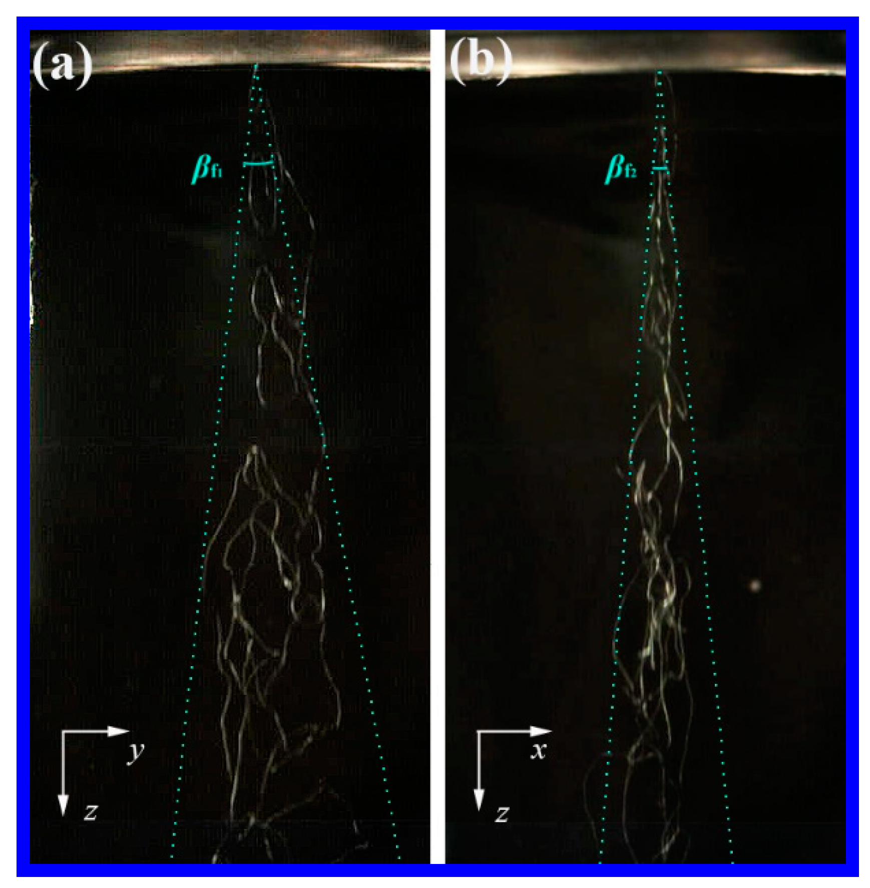
4.3. Fiber Path in Melt Blowing

Figure 11 shows the fiber paths below the melt-blown slot die. It is obviously that the cross-section of the fiber path in the x–y plane is not round (but more likely to be elliptical), the amplitude of the fiber path in the y–z plane is larger than that in the x–z plane. The envelope angle of the fiber path in the y–z plane, β_f1, is about 16.3°, while, the envelope angle in the x–z plane, β_f2, is 9.1°. It is worth noting that β_f1 = 16.3° is fairly consistent with the air diffused envelope angle, β = 17.1° in the y–z plane, indicating that the critical boundary of the air lateral diffusion might control the lateral fiber distribution during melt blowing, or at least they have a close relationship.

During melt blowing, fiber whipping occurs as soon as the polymer melts out from the orifice, according to Yarin’s theory [17], when the flow velocity incident on a jet, exceeds a critical velocity, a small disturbance of the jet will grow and develop into a bending instability. Figure 9 and Figure 10 provide an extra clue for initiating fiber whipping, fiber is driven directly by the lateral velocity all the time without critical velocity mentioned by Yarin [17]. In consideration of the high drag efficiency of lateral velocity on the fiber (shown in Figure 2), there are reasons to believe that the small lateral velocity still has a crucial effect on initiating instability or whipping of the polymeric fiber during melt blowing.

5. Conclusions

In this work, the necessity of measuring the lateral velocity in melt blowing was first theoretical verified. Then, the velocity direction of the air flow in slot-die melt blowing was measured using a dual-probe hot-wire anemometer, and the fiber path was captured by high-speed photography. The results of the air velocity direction show that there exists a critical boundary of air lateral diffusion in the y–z plane. However, the air flow in the x–z plane is a completely diffused field. In addition, the fluctuating signal of the velocity direction is also shown, which might be a reason for initiating fiber instability. Finally, the relationship between the air lateral diffusion and the fiber whipping path was compared and discussed.

This work provides an extra clue for initiating fiber whipping, the lateral velocity plays crucial effect on initiating instability or whipping of the polymeric fiber, even though it is much smaller than the vertical velocity. This work indicates that, the air lateral diffusion deserves to be further discovering for detailed melt-blown research.

References

1. Wang, H.; Zhang, Y.; Gao, H.P.; Jin, X.Y.; Xie, X.H. Composite Melt-Blown Nonwoven Fabrics with Large Pore Size as Li-Ion Battery Separator. Int. J. Hydrog. Energy 2016, 41, 324–330. [Google Scholar] [CrossRef]
2. Burger, C.; Hsiao, B.S.; Chu, B. Nanofibrous Materials and Their Applications. Annu. Rev. Mater. Res. 2006, 36, 333–368. [Google Scholar] [CrossRef]
3. Krutka, H.M.; Shambaugh, R.L.; Papavassiliou, D.V. Analysis of a Melt-Blowing Die: Comparison of CFD and Experiments. Ind. Eng. Chem. Res. 2002, 41, 5125–5138. [Google Scholar] [CrossRef]
4. Krutka, H.M.; Shambaugh, R.L.; Papavassiliou, D.V. Effects of Die Geometry on the Flow Field of the Melt-Blowing Process. Ind. Eng. Chem. Res. 2003, 42, 5541–5553. [Google Scholar] [CrossRef]
5. Krutka, H.M.; Shambaugh, R.L.; Papavassiliou, D.V. Effects of Temperature and Geometry on the Flow Field of the Melt Blowing Process. Ind. Eng. Chem. Res. 2004, 43, 4199–4210. [Google Scholar] [CrossRef]
6. Krutka, H.M.; Shambaugh, R.L.; Papavassiliou, D.V. Analysis of the Temperature Field from Multiple Jets in the Schwarz Melt Blowing Die Using Computational Fluid Dynamics. Ind. Eng. Chem. Res. 2006, 45, 5098–5109. [Google Scholar] [CrossRef]
7. Lee, Y.E.; Wadsworth, L.C. Fiber and Web Formation of Melt-Blown Thermoplastic Polyurethane Polymers. J. Appl. Polym. Sci. 2007, 105, 3723–3727. [Google Scholar] [CrossRef]
8. Chen, T. Study on the Air Drawing in Melt Blowing Nonwoven Process. Ph.D. Thesis, Donghua University, Shanghai, China, 2003. [Google Scholar]
9. Sun, Y.F.; Liu, B.W.; Wang, X.H.; Zeng, Y.C. Air-Flow Field of the Melt-Blowing Slot Die Via Numerical Simualtion and Multiobjective Genetic Algorithms. J. Appl. Polym. Sci. 2011, 122, 3520–3527. [Google Scholar] [CrossRef]
10. Wang, Y.D.; Wang, X.H. Experimental Investigation into a New Melt-Blowing Die for Dual Rectangular Jets. Adv. Mater. Res. 2014, 945–949, 270–273. [Google Scholar] [CrossRef]
11. Xie, S.; Han, W.L.; Jiang, G.J.; Chen, C. Turbulent Air Flow Field in Slot-Die Melt Blowing for Manufacturing Microfibrous Nonwoven Materials. J. Mater. Sci. 2018, 53, 6991–7003. [Google Scholar] [CrossRef]
12. Hassan, M.A.; Anantharamaiah, N.; Khan, S.A.; Pourdeyhimi, B. Computational Fluid Dynamics Simulations and Experiments of Meltblown Fibrous Media: New Die Designs to Enhance Fiber Attenuation and Filtration Quality. Ind. Eng. Chem. Res. 2016, 55, 2049–2058. [Google Scholar] [CrossRef]
13. Chhabra, R.C.; Shambaugh, R.L. Experimental Measurements of Fiber Threadline Vibrations in the Melt-Blowing Process. Ind. Eng. Chem. Res. 1996, 35, 4366–4374. [Google Scholar] [CrossRef]
14. Bresee, R.R.; Qureshi, U.A. Influence of Processing Conditions on Melt Blown Web Structure: Part IV-Fiber Diameter. Int. Nonwovens J. 2006, 1, 32–46. [Google Scholar]
15. Xie, S.; Zeng, Y.C. Online Measurement of Fiber Whipping in the Melt-Blowing Process. Ind. Eng. Chem. Res. 2013, 52, 2116–2122. [Google Scholar] [CrossRef]
16. Reneker, D.H.; Yarin, A.L. Electrospinning Jets and Polymer Nanofibers. Polymer 2008, 49, 2387–2425. [Google Scholar] [CrossRef]
17. Entov, V.M.; Yarin, A.L. The Dynamics of Thin Liquid Jets in Air. J. Fluid Mech. 1984, 140, 91–111. [Google Scholar] [CrossRef]
18. Rao, R.S.; Shambaugh, R.L. Vibration and Stability in the Melt Blowing Process. Ind. Eng. Chem. Res. 1993, 32, 3100–3111. [Google Scholar] [CrossRef]
19. Marla, V.T.; Shambaugh, R.L. Three-Dimensional Model of the Melt-Blowing Process. Ind. Eng. Chem. Res. 2003, 42, 6993–7005. [Google Scholar] [CrossRef]
20. Uyttendaele, M.A.; Shambaugh, R.L. Melt Blowing: General Equation Development and Experimental Verification. AICHE J. 1990, 36, 175–186. [Google Scholar] [CrossRef]
21. Ellison, C.J.; Phatak, A.; Giles, D.W.; Macosko, C.W.; Bates, F.S. Melt Blown Nanofibers: Fiber Diameter Distributions and Onset of Fiber Breakup. Polymer 2007, 48, 3306–3316. [Google Scholar] [CrossRef]
22. Tan, D.H.; Zhou, C.F.; Ellison, C.J.; Kumar, S.; Macosko, C.W.; Bates, F.S. Meltblown Fibers: Influence of Viscosity and Elasticity on Diameter Distribution. J. Non-Newton. Fluid Mech. 2010, 165, 892–900. [Google Scholar] [CrossRef]
23. Zhou, C.F.; Tan, D.H.; Janakiraman, A.P.; Kumar, S. Modeling the Melt Blowing of Viscoelastic Materials. Chem. Eng. Sci. 2011, 66, 4172–4183. [Google Scholar] [CrossRef]
24. Chung, C.; Kumar, S. Onset of Whipping in the Melt Blowing Process. J. Non-Newton. Fluid Mech. 2013, 192, 37–47. [Google Scholar] [CrossRef]
25. Tan, D.H.; Herman, P.K.; Janakiraman, A.; Bates, F.S.; Kumar, S.; Macosko, C.W. Influence of Laval Nozzles on the Air Flow Field in Melt Blowing Apparatus. Ind. Eng. Chem. Res. 2012, 80, 342–348. [Google Scholar] [CrossRef]
26. Wang, Z.F.; Espín, L.; Bates, F.S.; Kumar, S.; Macosko, C.W. Water Droplet Spreading and Imbibition on Superhydrophilic Poly(Butylene Terephthalate) Melt-Blown Fiber Mats. Chem. Eng. Sci. 2016, 146, 104–114. [Google Scholar] [CrossRef]
27. Soltani, I.; Macosko, C.W. Influence of Rheology and Surface Properties on Morphology of Nanofibers Derived from Islands-In-The-Sea Meltblown Nonwovens. Polymer 2018, 145, 21–30. [Google Scholar] [CrossRef]
28. Yarin, A.L.; Sinha-Ray, S.; Pourdeyhimi, B. Meltblowing: Multiple Polymer Jets and Fiber-Size Distribution and Lay-Down Patterns. Polymer 2011, 52, 2929–2938. [Google Scholar] [CrossRef]
29. Sinha-Ray, S.; Yarin, A.L.; Pourdeyhimi, B. Prediction of Angular and Mass Distribution in Meltblown Polymer Lay-Down. Polymer 2013, 54, 860–872. [Google Scholar] [CrossRef]
30. Sinha-Ray, S.; Yarin, A.L.; Pourdeyhimi, B. Meltblown Fiber Mats and Their Tensile Strength. Polymer 2014, 55, 4241–4247. [Google Scholar] [CrossRef]
31. Sinha-Ray, S.; Sinha-Ray, S.; Yarin, A.L.; Pourdeyhimi, B. Theoretical and Experimental Investigation of Physical Mechanisms Responsible for Polymer Nanofiber Formation in Solution Blowing. Polymer 2015, 56, 452–463. [Google Scholar] [CrossRef]
32. Ghosal, A.; Ray-Sinha, S.; Yarin, A.L.; Pourdeyhimi, B. Numerical Prediction of Effect of Uptake Velocity on Three-Dimensional Structure, Porosity and Permeability of Meltblown Nonwoven Laydown. Polymer 2016, 85, 19–27. [Google Scholar] [CrossRef]
33. Sun, Y.F.; Zeng, Y.C.; Wang, X.H. Three-Dimensional Model of Whipping Motion in the Processing of Microfibers. Ind. Eng. Chem. Res. 2011, 50, 1099–1109. [Google Scholar] [CrossRef]
34. Xie, S.; Zeng, Y.C.; Han, W.L.; Jiang, G.J. An Improved Lagrangian Approach for Simulation Fiber Whipping in Slot-Die Melt Blowing. Fibers Polym. 2017, 18, 525–532. [Google Scholar] [CrossRef]
35. Matsui, M. Air Drag on a Continuous Filaments in Melt Spinning. Trans. Soc. Rheol. 1976, 20, 465–473. [Google Scholar] [CrossRef]
36. Majumdar, B.M.; Shambaugh, R.L. Air Drag on Filaments in the Melt Blowing Process. J. Rheol. 1990, 34, 591–601. [Google Scholar] [CrossRef]
37. Ju, Y.D.; Shambaugh, R.L. Air Drag on Fine Filaments at Oblique and Normal Angles to the Air Stream. Polym. Eng. Sci. 1994, 34, 958–964. [Google Scholar] [CrossRef]
38. Beard, J.H.; Shambaugh, R.L.; Shambaugh, B.R.; Schmidtke, D.W. On-Line Measurement of Fiber Motion During Melt Blowing. Ind. Eng. Chem. Res. 2007, 46, 7340–7352. [Google Scholar] [CrossRef]
Figure 1. (a) Schematic of commercial slot-die melt-blown process. (b) The microfibrous nonwovens produced by melt blowing. (c) Schematic of a fiber fragment near the die and the air velocity applied on it.
Polymers 11 00788 g001
Figure 2. Fp, FN with respect to θ under the same assumption.
Polymers 11 00788 g002
Figure 3. (a) Section view (b) top view of the slot die used in this work.
Polymers 11 00788 g003
Figure 4. (a) Schematic of the constant temperature anemometer (CTA) device and melt-blown die during air velocity direction measurement. The shown air flow field is obtained by Computational Fluid Dynamics (CFD). (b) The structures of the dual-wire probe.
Polymers 11 00788 g004
Figure 5. (a) Schematic of devices for the directional calibration of the CTA. Directional calibration was performed by exposing the probe (wires) to a known air velocity from different angles. (b) Calibration angle and its two corresponding voltages for the dual wires.
Polymers 11 00788 g005
Figure 6. The directional angle between the z-axis and the resultant velocity in the y–z plane at different position along lines 1–4. Lines 1–4 were defined as described in Section 3.2.
Polymers 11 00788 g006
Figure 7. The angle down from the z-axis of the resultant air velocity in the x–z plane at different positions along lines 5–8.
Polymers 11 00788 g007
Figure 8. The fluctuant signals of the angle between the z-axis and the resultant velocity in the y–z plane at the (y, z) positions of (a) (2 mm, 6 mm), (b) (5 mm, 6 mm), (c) (10 mm, 6 mm), (d) (20 mm, 6 mm).
Polymers 11 00788 g008
Figure 9. The distribution of lateral velocity, vy, along lines 1–4 of y = 2, 5, 10, and 20 mm, in the corresponding y–z plane. A represents the lateral diffusion region, B represents the lateral back-diffusion region.
Polymers 11 00788 g009
Figure 10. The distribution of lateral velocity, vx, along lines 5–8 of x = 2, 5, 10, and 20 mm, in the corresponding x–z plane.
Polymers 11 00788 g010
Figure 11. The fiber paths below the melt-blown slot die. (a) The fiber path in the y–z plane. (b) The fiber path in the x–z plane. The corresponding size of each image is 62.5 mm × 130 mm.
Polymers 11 00788 g011