Appendix A.1. Estimation of the Laser Penetration Time
In
Section 3.1, the laser penetration time could be calculated as follows:
In Reference [
20], the effective total interaction time,
, could be calculated as follows:
where
,
,
, and
were the laser power, the process-depth, the spot area, and the sublimation temperature, respectively.
The two equations are based on the energy balance in the process of the carbon fiber sublimation in which the heat diffuse along the fibers is neglected. In Equation (3), the thickness of the specimen
represents the
of Equation (A1) and the
represents the
of Equation (A1). In the reference, the laser intensity (power density)
. In this study, the Gaussian laser intensity could be written as:
where
,
,
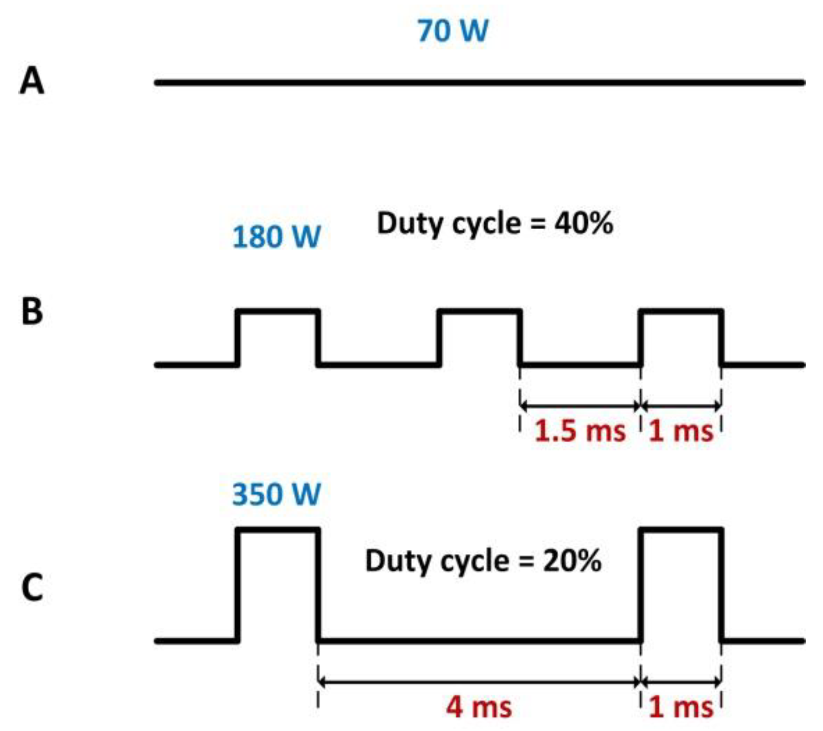
were the distance from the spot center, the spot radius, and the average laser intensity in the spot. The pulse peak power density of the ms laser and the mean power density of the CW laser as shown in
Table 2 were calculated with the expression:
.
From Equation (A2), it could be found that the maximum value of the laser intensity (
) was in the center of the laser spot (
). In CW laser mode, the duty cycle
= 1 and
. Therefore, the laser intensity in the center of the laser spot kept
. In the pulse laser mode,
was a periodic function of square wave, as shown below:
where
was zero or a positive integer and the pulse duration
. Additionally, the duty cycle
was as shown in
Table 2. Therefore, the average laser intensity in the center of the laser spot could be calculated as
. So
could represent the
of Equation (A1). Therefore, Equation (3) could be used to estimate the laser penetration time in
Section 3.1.
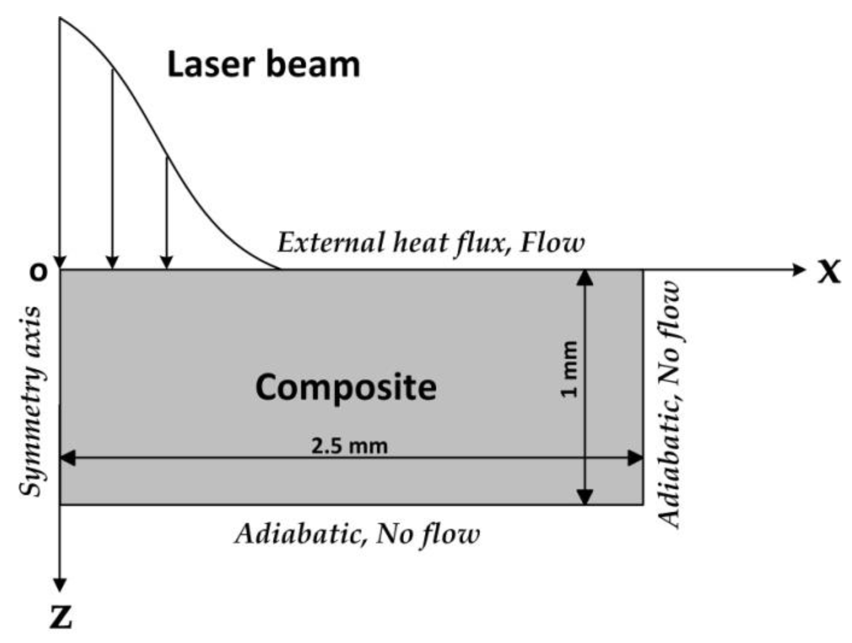
Appendix A.2. Model Formulation for the Internal Gas Pressure
For
Section 4.1, in order to predict the temperature field and the internal gas pressure in the composite during the laser drilling, a two-dimensional axisymmetric finite element model was established. To simplify the calculation, the composite could be considered a homogeneous anisotropic block [
24,
25]. The schematic of the model is shown in
Figure A1.
Additionally, some assumptions were adopted, as follows:
- (1)
The laser energy was completely absorbed on the surface of the composite.
- (2)
The possible oxidation reaction and the material erosion on the composite surface were neglected.
- (3)
The polymer matrix degraded into the carbon residue and pyrolysis gas directly via heating.
- (4)
The pyrolysis gas was chemically non-reactive and the ideal gas equation of state could be used.
- (5)
The pyrolysis gas was always in thermal equilibrium with the nearby solid.
- (6)
The volume change and the thermal expansion of the material were neglected.
Therefore, during the laser drilling, the polymer matrix that experienced pyrolysis contained three types of components: polymer resin, decomposition gases, and carbon residue (char). The
of the composite could be written as [
26]:
where
represented the volume fraction of component
i in a unit volume.
was given with reference to the mass of component
i (
) and the constant density of component
i (
) by considering
In addition,
could be neglected because
was much smaller than
,
, and
The quantity
is the ratio of the completely pyrolyzed matrix to the virgin matrix as follows:
where the subscripts ‘
’ and ‘
’ denote the original state and the end state, respectively.
was used [
27]. Hence, the mass transforming relationship of the polymer resin and char could be given by:
The decomposition gases volume fraction
could be calculated with the following expression:
The initial volume fraction of gas was assumed to be 0.003 in this model.
The governing equation of the thermal transport through the composite could be written as follows [
24,
25,
28]:
where
and
were the heat of decomposition and the gas velocity, respectively. The second term on the right-hand side of Equation (A9) represents the energy consumption due to polymer pyrolysis. The third term on the right-hand side represents a contribution of the gas convection to the internal energy. The thermal conductivity perpendicular to the incident laser beam could be considered with the following expression [
18,
24]:
The thermal conductivity in the thickness direction
is shown in
Table A1 [
29]. Additionally, some material thermal parameters used in the model are shown in
Table 1, and the others are shown in
Table A2 [
18,
24].
Table A1.
Carbon-phenolic thermal conductivity perpendicular to the fiber axis.
Table A1.
Carbon-phenolic thermal conductivity perpendicular to the fiber axis.
| |
|---|
| 300 | 0.0056 |
| 422 | 0.0076 |
| 533 | 0.0085 |
| 811 | 0.0054 |
| 1367 | 0.0077 |
| 1922 | 0.0099 |
| 3500 | 0.0222 |
Table A2.
Some thermal parameters of the components in the composite.
Table A2.
Some thermal parameters of the components in the composite.
| Parameter | Symbol | Value | Units |
|---|
| Thermal conductivity of the polymer resin [18] | | 0.2 | W/(m·K) |
| Density of the polymer resin [24] | | 900 | kg/m3 |
| Heat capacity of the polymer resin [24] | | 2500 | J/(kg·K) |
| Thermal conductivity of the carbon residue [24] | | 0.2 | W/(m·K) |
| Density of the carbon residue [24] | | 1300 | kg/m3 |
| Heat capacity of the carbon residue [24] | | 1589 | J/(kg·K) |
| Thermal conductivity of the pyrolysis gas [24] | | 0.025 | W/(m·K) |
| Density of the pyrolysis gas [24] | | 1.997 | kg/m3 |
| Heat capacity of the pyrolysis gas [24] | | 720 | J/(kg·K) |
| The heat of decomposition [24] | | 9 × 10⁵ | J/kg |
| Thermal conductivity of the carbon fiber parallel to the fiber axis [18] | | 50 | W/(m·K) |
| Thermal conductivity of the carbon fiber perpendicular to the fiber axis [18] | | 5 | W/(m·K) |
| Density of the carbon fiber [18] | | 1850 | kg/m3 |
| Heat capacity of the carbon fiber [18] | | 710 | J/(kg·K) |
In
Table A2, the parameters of CO
2 were used as the thermal parameters of the pyrolysis gases.
The rate of polymer resin pyrolysis could be roughly described using an Arrhenius equation with the form of [
24,
25]:
where
,
,
,
were the pre-exponential factor, the reaction order, the activation energy, and the ideal gas constant, respectively. In the model,
is 3.15 × 10
11 s
−1,
is 1.344,
is 1.8173 × 10
5 J/mol, and
is 8.31 J/(mol·K) [
24].
The relationship of the mass conservation of the internal gas was given by the continuity equation as follows:
The left-hand side of Equation (A12) represents the mass of the gases produced by matrix decomposition. The first term on the right-hand of Equation (A12) represents the gas mass convection through the porous material. The second term on the right-hand is the time rate of the change of gas storage in the composite. This term is commonly negligible. And
was given by the Darcy filtration law as follows [
24,
25,
30]:
where
,
, and
were the permeability, the gas kinematic viscosity, and the gas pressure inside the decomposing composite, respectively. Additionally, the calculation equation of the permeability could be written as follows:
where
was the diameter of a single carbon fiber, defined as 6
and
C = 144 [
27,
31]. The kinematic viscosity that was used in the model was assumed to be 3 × 10
−5 Pa·s. Because the trapped gas was assumed to be an ideal gas, the gas pressure could be calculated with the following expression:
where
was used as the average molecular weight of CO
2 44 g/mol.
In addition, when the temperature of the composite material exceeded the vaporization point of carbon (
= 3600 K), a simplified sublimation mechanism was used, as shown below:
where the latent heat of carbon sublimation
was added to the equivalent heat capacity
of the composite material [
32,
33]. Here,
K and
K. To simulate the process of laser irradiation on the new composite surface after the original surface ablated, a large thermal conductivity in the thickness direction was used, as shown below:
In this model, 5 × 10³ W/(m·K). The , , , and terms could be replaced with , , , and , respectively. Then, the numerical model could describe the two processes of the thermal decomposition in the composite and the sublimation on the surface at the same time.
Because the pyrolysis gases did not absorb and shield the laser energy, the laser energy received by the composite surface was equal to the output energy of the laser. Although the pyrolysis gases that were released from the composite surface changed the ambient temperature and the convective heat transfer on the surface [
29,
34,
35,
36], the effect of the pyrolysis gases on the surface heat exchange was much less than the effect of the absorbed laser fluence in the model was. Therefore, the boundary conditions of the laser drilling process could be represented as follows:
where the spot radius
, the heat transfer coefficient
, the emissivity of carbon-phenolic
, and the Stefan-Boltzmann constant
.
is the ambient temperature and
is the temperature of the irradiated surface. The first term on the right-hand side of Equation (A22) represents the laser heat fluence with a Gauss distribution in space. The second term on the right-hand side of Equation (A22) represents the air convection cooling on the surface, and the third term on the right-hand side of Equation (A22) represents the heat exchange between the heated surface and surroundings.
The above mathematical model was achieved numerically through the finite element method (FEM) with the help of the business software COMSOL 4.2. In COMSOL 4.2, Equations (A9),(A11),(A12) could be calculated using the Heat Transfer Module, the Chemical Reaction Engineering Module, and the Computational Fluid Dynamics (CFD) Module, respectively. These three main governing equations were coupled by the variables of
,
, and
. The geometry of 2.5 mm × 1 mm, as shown in
Figure A1, was divided by a non-uniform mapped mesh. The external heat flux defined by Equation (A22) was positioned at the top surface (
z = 0), which generated a large temperature gradient near the laser center. Hence, the distribution of the elements in the mesh was dense at the laser radiation area and the distribution gradually became sparse from the Point o (0,0) to the outside in a fixed ratio. In this model, the minimum spatial element size was less than 9 × 10
−7 m. The edge boundaries of
x = 2.5 mm and
z = 1 mm were adiabatic (Equation (A24)). The pyrolysis gases could only flow out from the edge boundary of
z = 0. The initial temperature
was assumed to be 300 K, and the initial internal gas pressure
was assumed to be 1 atm. The constant ambient temperature
was assumed to be 300 K, and the constant ambient pressure
was assumed to be 1 atm. The initial volume fractions of the composite components were
,
, and
.
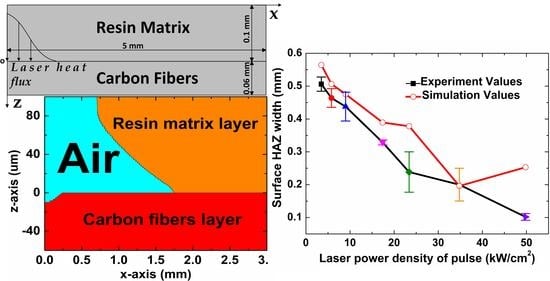
Appendix A.3. Model Formulation for the Entrance Hole Diameter and the Surface HAZ Width
For
Section 4.2, to accurately predict the entrance hole diameter and the surface HAZ, a new geometric model was proposed, as shown in
Figure A2. In this model, the resin matrix layer with a 0.1 mm thickness and the carbon fibers layer with a 0.06 mm thickness were separated. The Point o (0,0) was at the interface of the two layers, as shown in
Figure A2.
In the resin matrix layer, the governing equations were simplified as follows:
In the carbon fibers layer, the governing equations were simplified as follows:
This model only considered the entrance hole diameter and the surface HAZ width, so the pyrolysis process of the polymer resin could be neglected. Therefore, the numerical model only needed to use the Heat Transfer Module of COMSOL. Additionally, because the epoxy resin was transparent for the NIR laser [
8,
38] and the absorption depth of the 1064 nm laser inside of carbon fiber varied in the range of 74 to 270 nm [
39,
40], the laser energy that was absorbed at the upper surface of the carbon fibers layer was considered in this model. Thus, the boundary conditions could be written as follows:
In addition, the distribution of elements in the mesh was dense at the boundary of
z = 0, and the distribution gradually became sparse from the laser center of the interface to the outside in a fixed ratio. In this model, the minimum spatial element size was less than 2.5 × 10
−7 m. The initial temperature
and the constant ambient temperature
were assumed to be 300 K. In the resin matrix layer,
. In the carbon fibers layer,
. And the other calculation parameters were shown in
Table 1,
Table A1 and
Table A2.
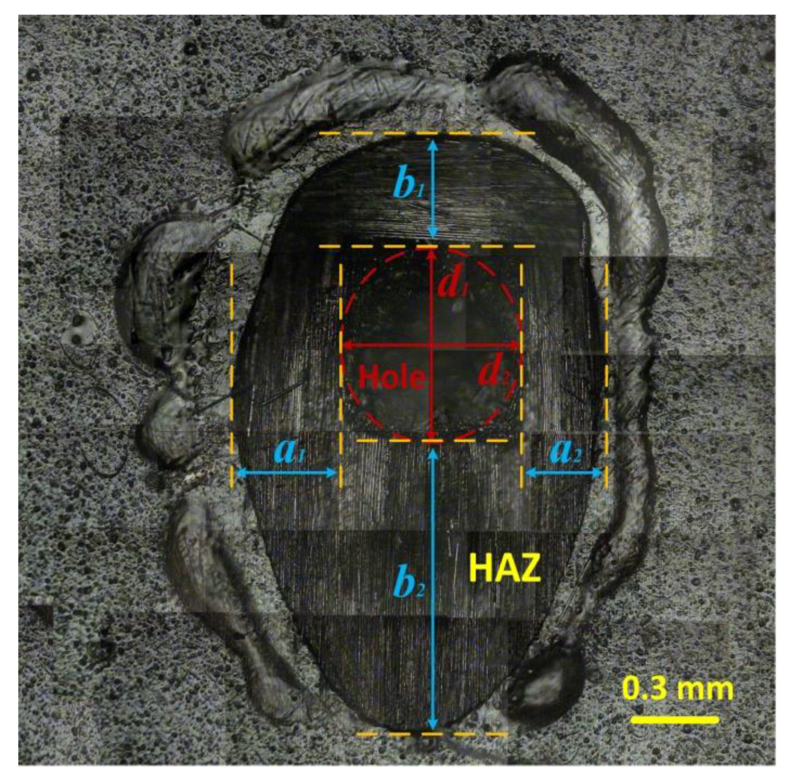
In all of the calculation time, the entrance hole diameter from the numerical simulation was defined as follows:
And the surface HAZ width from the numerical simulation was defined as follows:

 ,
, 


