Author Contributions
Conceptualization, J.V. and R.D.; methodology, J.V.; validation, J.R. and J.H.; formal analysis, J.V.; investigation, J.V.; resources, R.D.; data curation, J.H.; writing—original draft preparation, J.V.; writing—review and editing, M.K.; visualization, J.V.; supervision, R.D. and M.K.; project administration, R.R.; funding acquisition, R.R. All authors have read and agreed to the published version of the manuscript.
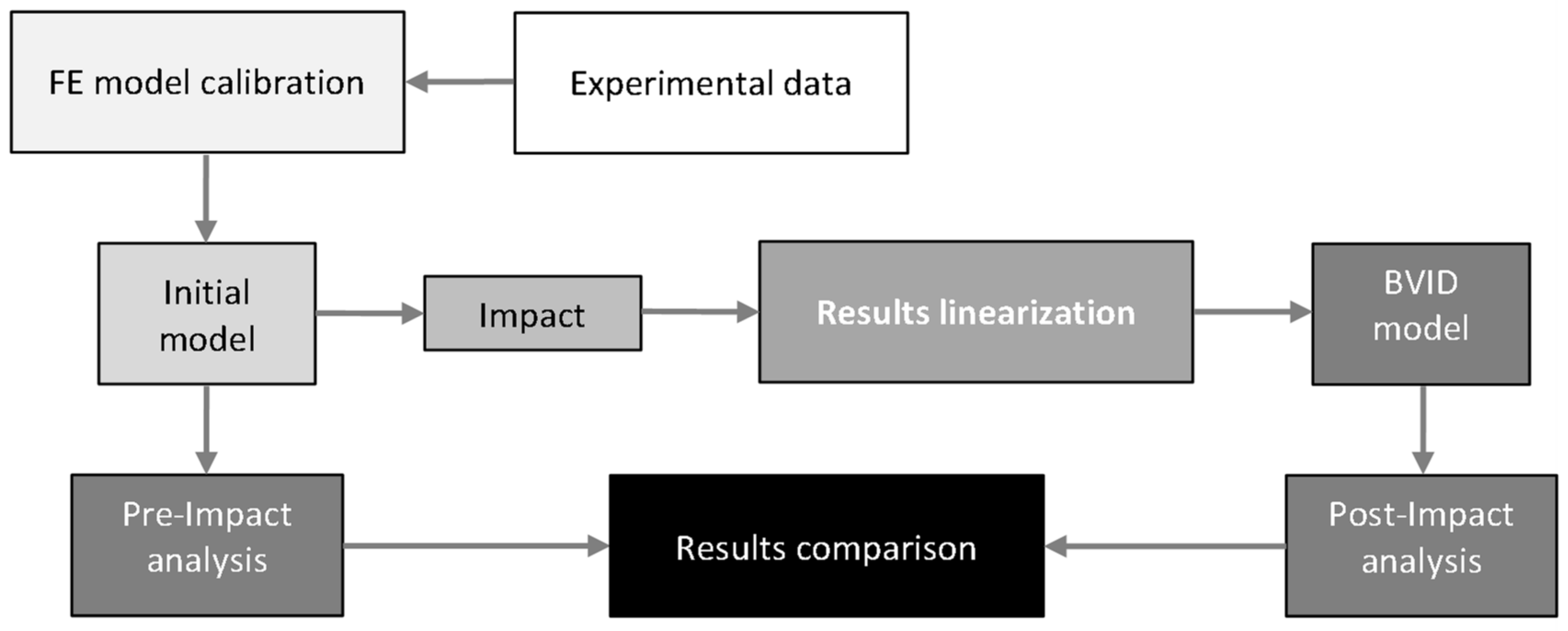
Figure 1.
Workflow schema.
Figure 1.
Workflow schema.
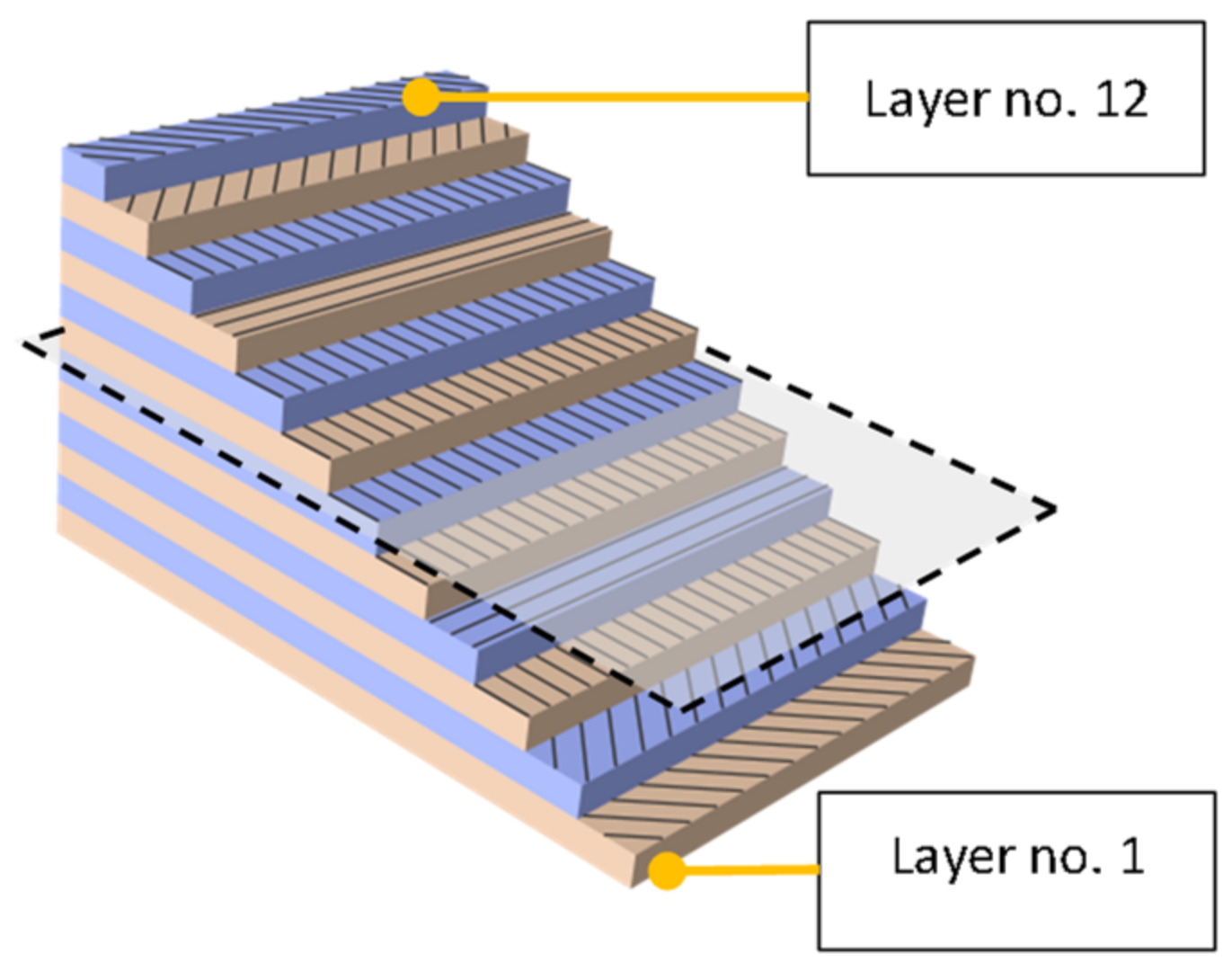
Figure 2.
Ply-by-ply model description.
Figure 2.
Ply-by-ply model description.
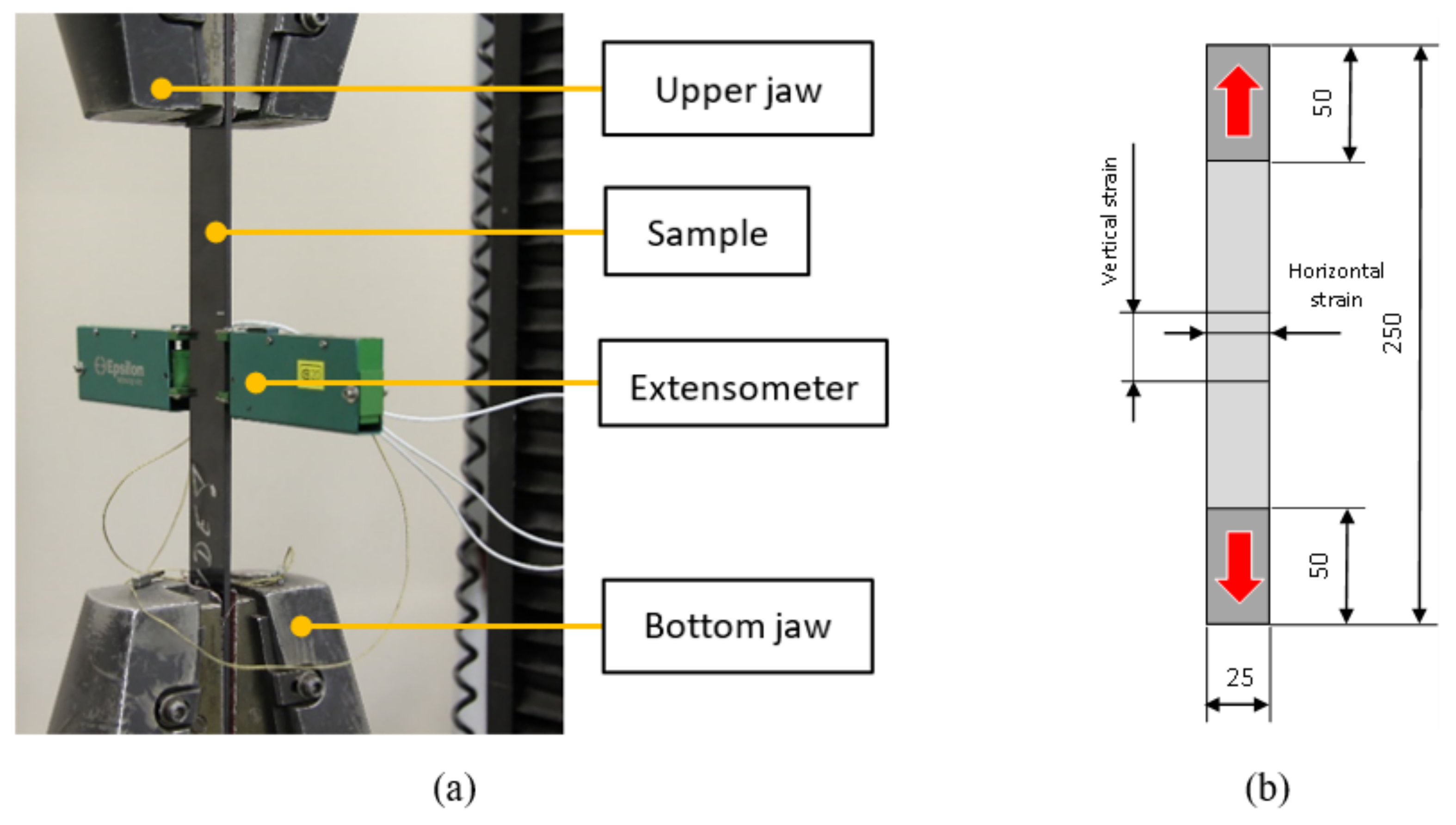
Figure 3.
Tensile test; Experiment (a); Tensile sample (b).
Figure 3.
Tensile test; Experiment (a); Tensile sample (b).
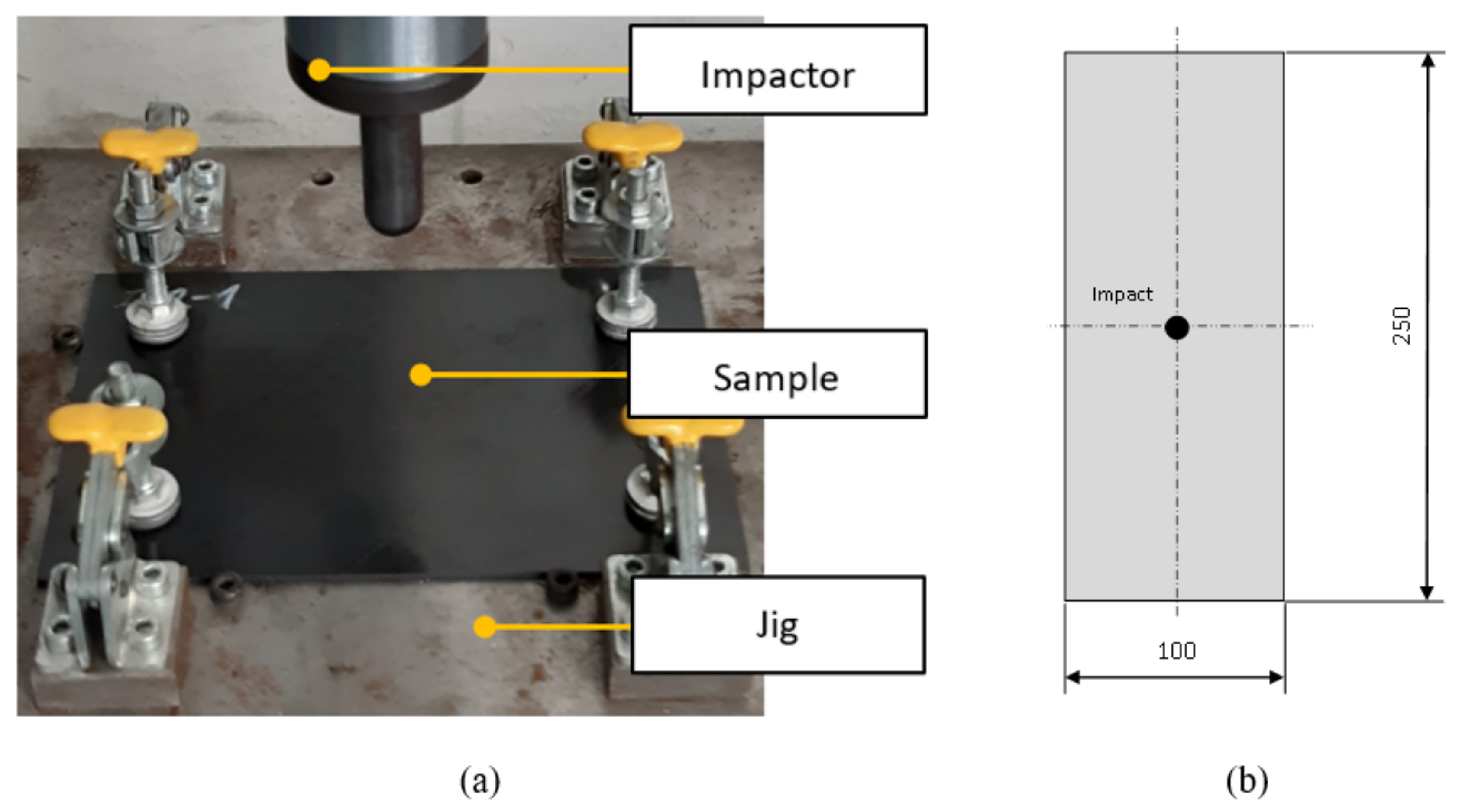
Figure 4.
Impact on the specimen; Experiment (a); Impact sample (b).
Figure 4.
Impact on the specimen; Experiment (a); Impact sample (b).
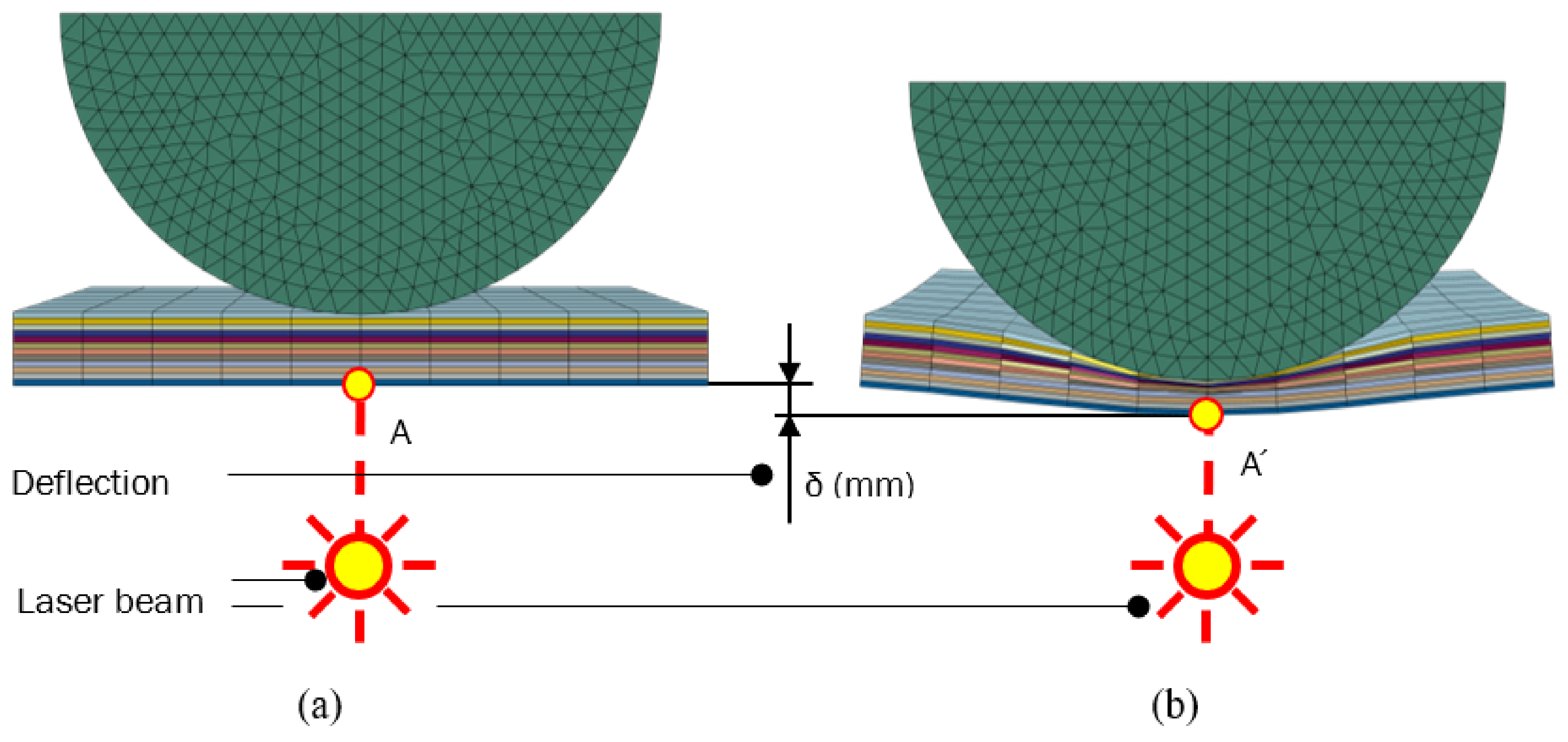
Figure 5.
Deflection under the impactor from the simulation results; Initial state of impact (a); Maximum plate displacement under impactor (b).
Figure 5.
Deflection under the impactor from the simulation results; Initial state of impact (a); Maximum plate displacement under impactor (b).
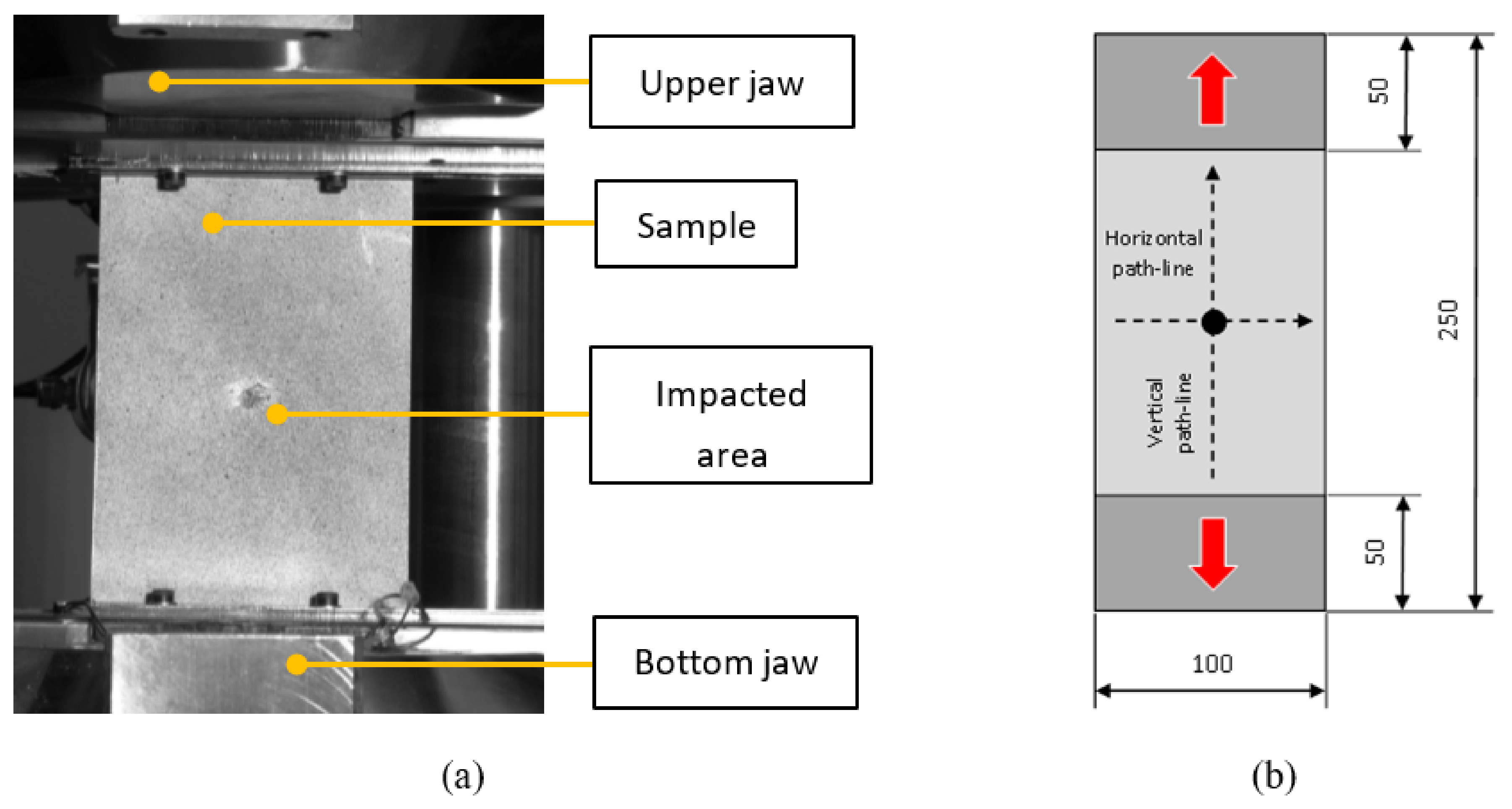
Figure 6.
Post-impact tensile test; Experiment (a); Sample with paths and dimensions (b).
Figure 6.
Post-impact tensile test; Experiment (a); Sample with paths and dimensions (b).
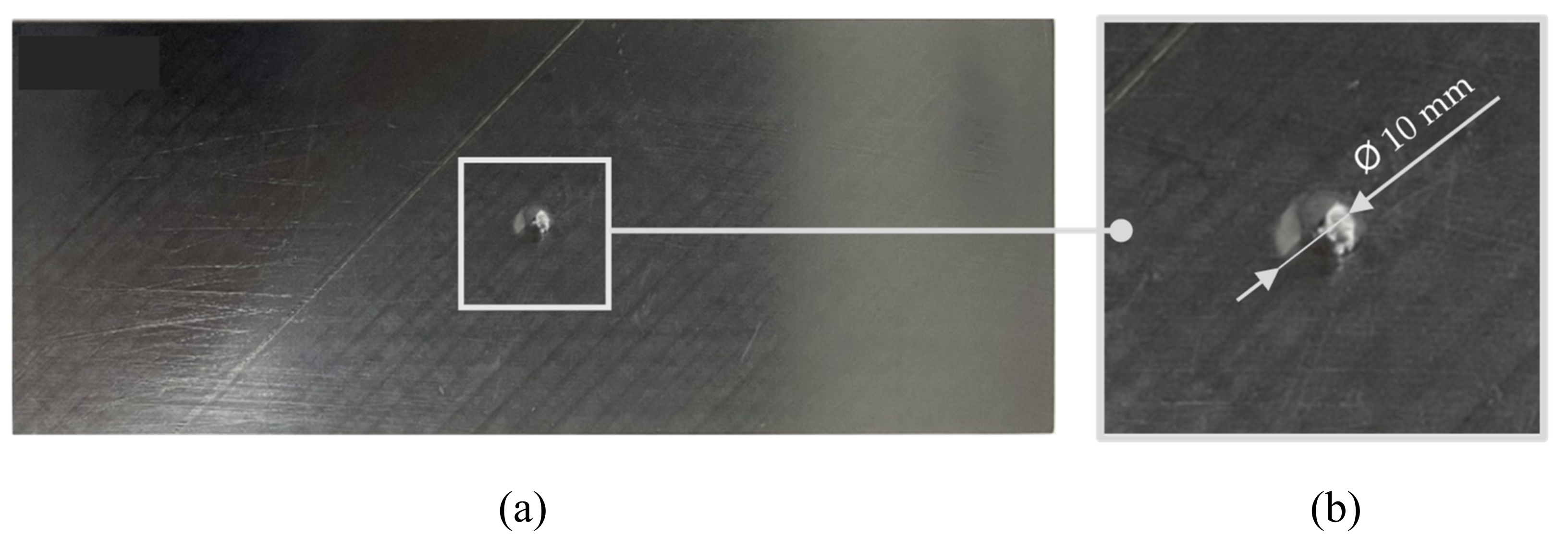
Figure 7.
Specimen after impact E = 10 J; Overall specimen view (a); Detailed view (b).
Figure 7.
Specimen after impact E = 10 J; Overall specimen view (a); Detailed view (b).
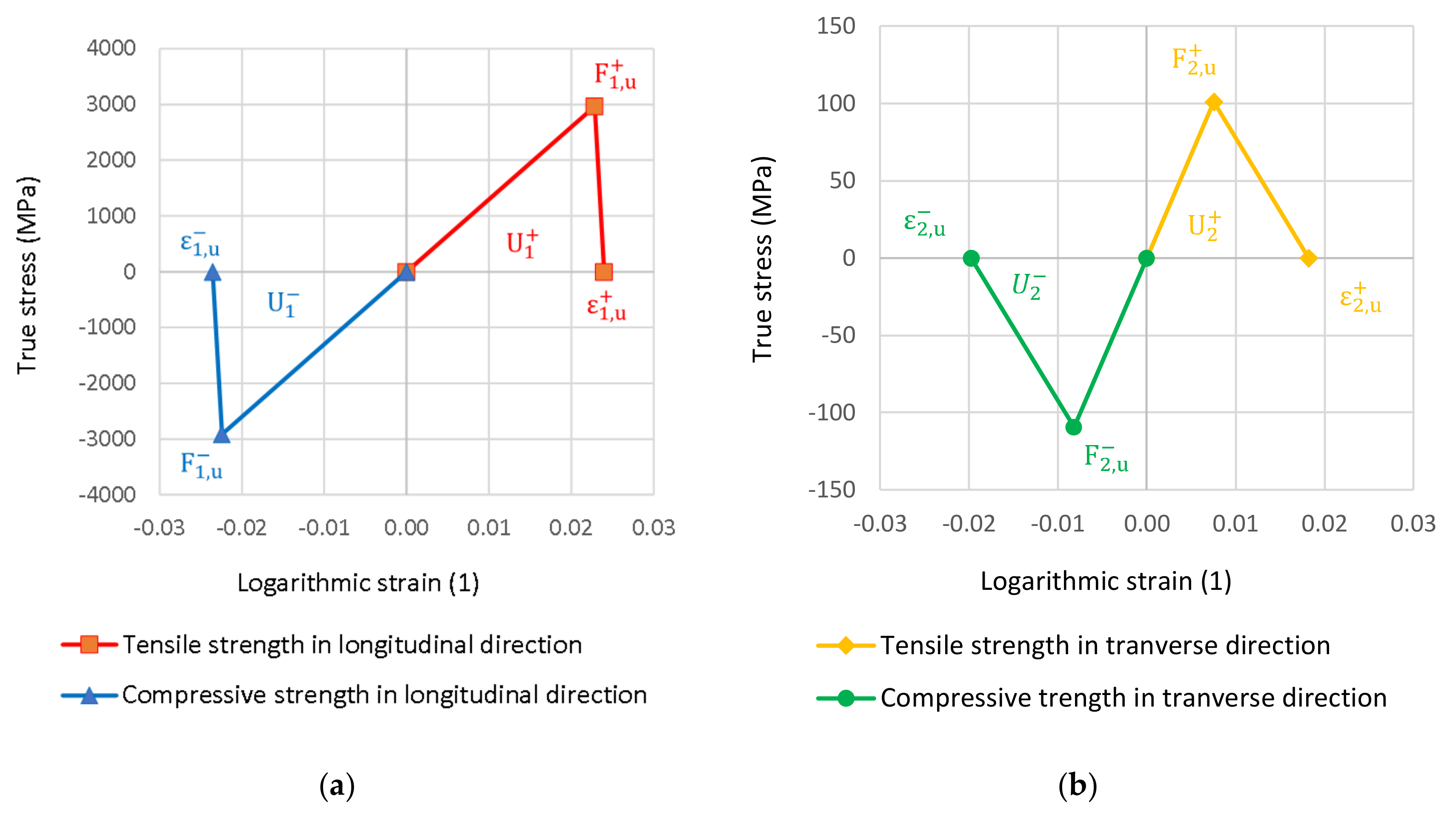
Figure 8.
Hashin damage diagram in longitudinal (a) and transverse laminate (b) direction.
Figure 8.
Hashin damage diagram in longitudinal (a) and transverse laminate (b) direction.
Figure 9.
Force–strain FEM tensile sample response.
Figure 9.
Force–strain FEM tensile sample response.
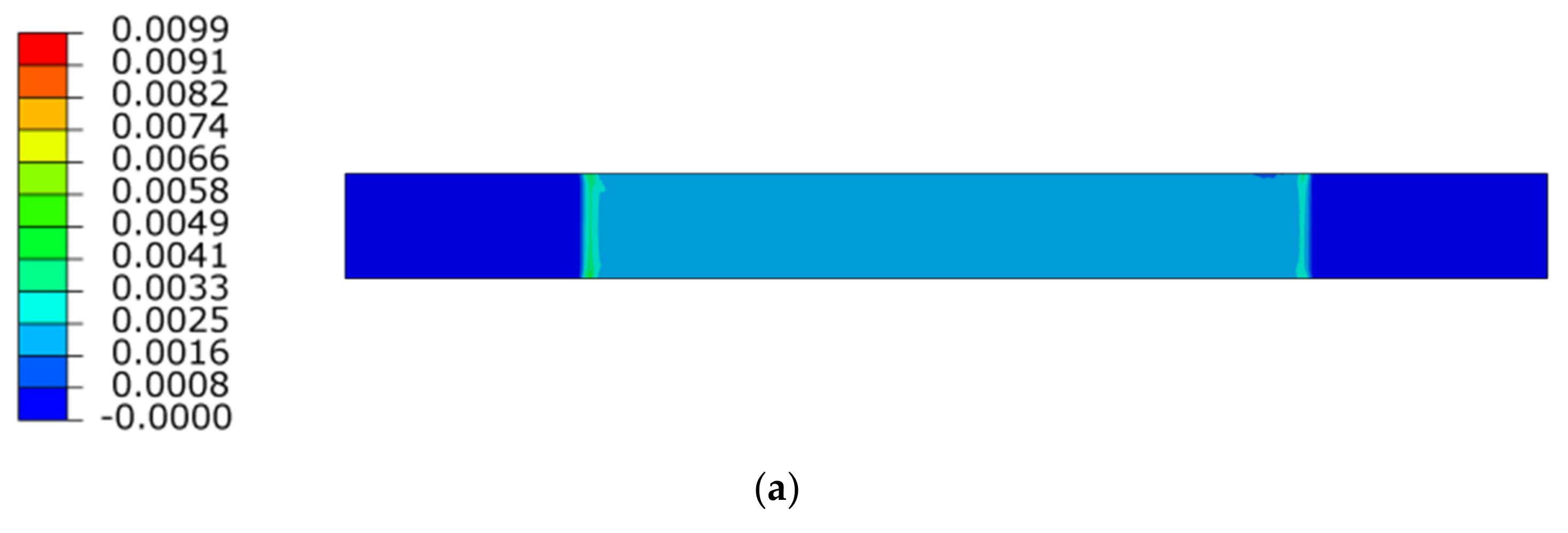
Figure 10.
Principal strain field distribution, Vertical (a), Horizontal (b).
Figure 10.
Principal strain field distribution, Vertical (a), Horizontal (b).
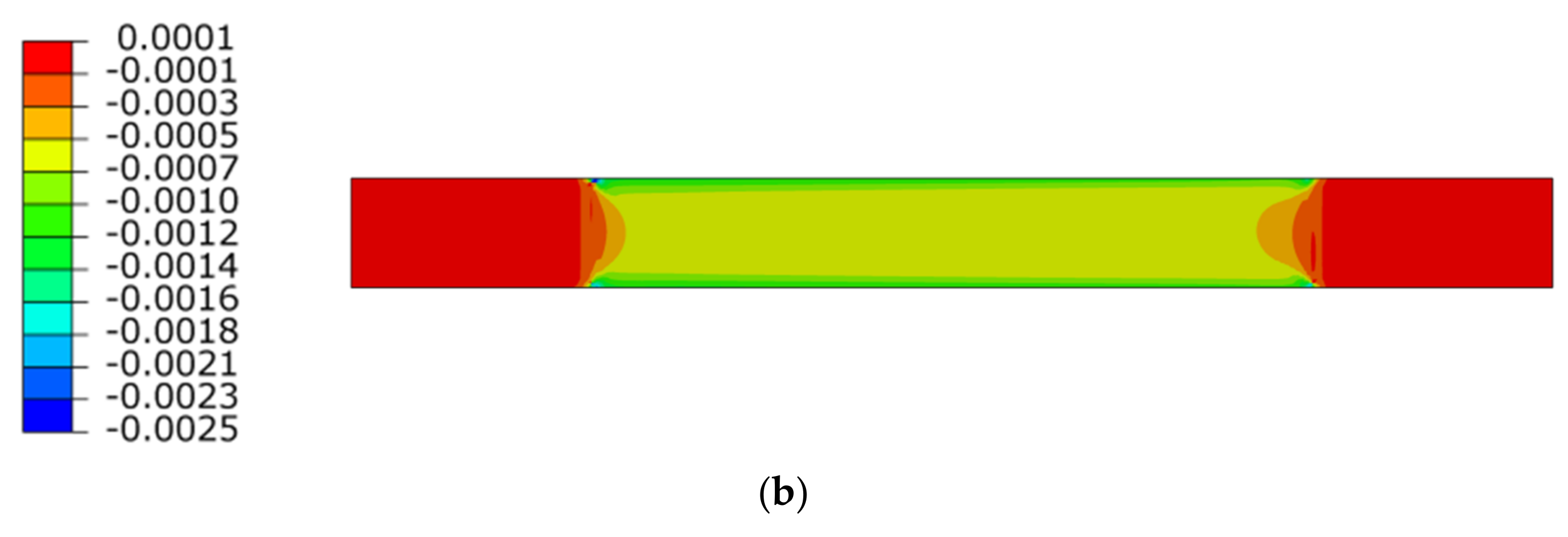
Figure 11.
Damage level of the specimen; Crack initiation from the FE model (a), Final damage from the FE model (b), Damage from the experiment (c).
Figure 11.
Damage level of the specimen; Crack initiation from the FE model (a), Final damage from the FE model (b), Damage from the experiment (c).
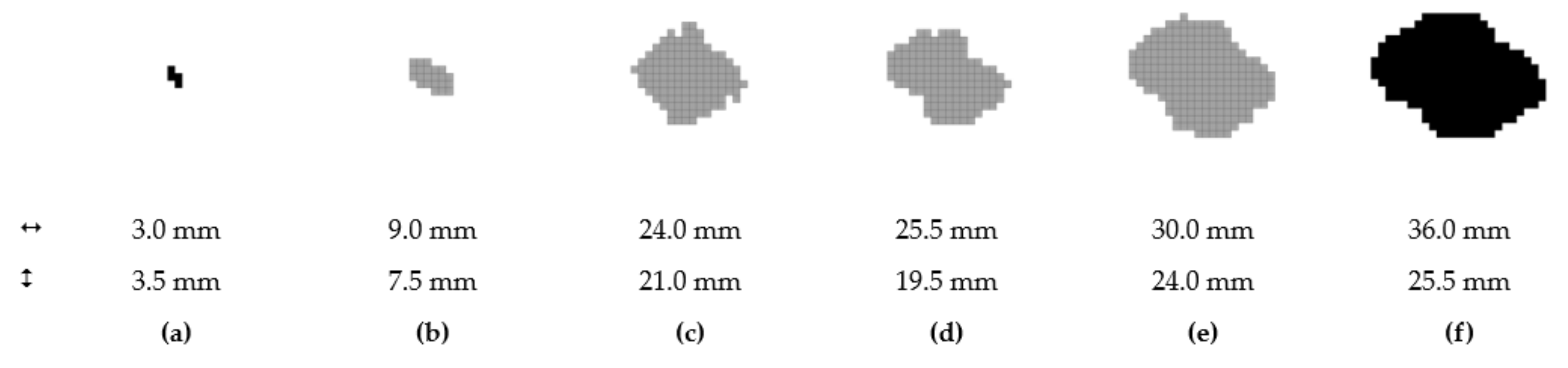
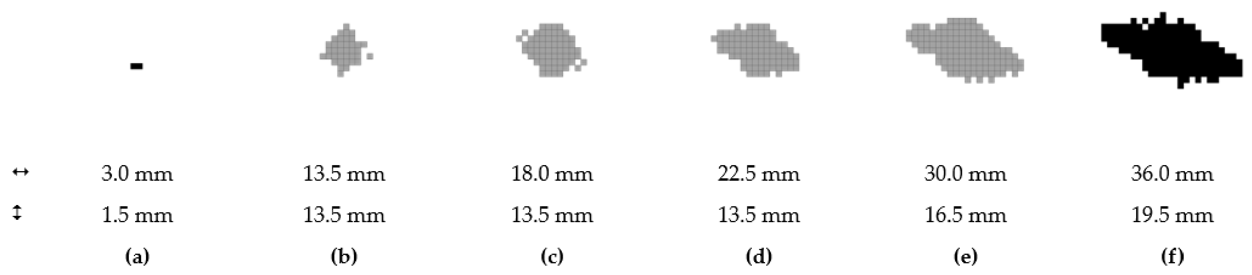
Figure 12.
Damaged area at layer no. 1; 0.5 J (a); 1.0 J (b); 2.5 J (c); 5.0 J (d); 7.5 J (e); 10.0 J (f).
Figure 12.
Damaged area at layer no. 1; 0.5 J (a); 1.0 J (b); 2.5 J (c); 5.0 J (d); 7.5 J (e); 10.0 J (f).
Figure 13.
Area damaged from impact; layer no. 12; 0.5 J (a); 1.0 J (b); 2.5 J (c); 5.0 J (d); 7.5 J (e); 10.0 J (f).
Figure 13.
Area damaged from impact; layer no. 12; 0.5 J (a); 1.0 J (b); 2.5 J (c); 5.0 J (d); 7.5 J (e); 10.0 J (f).
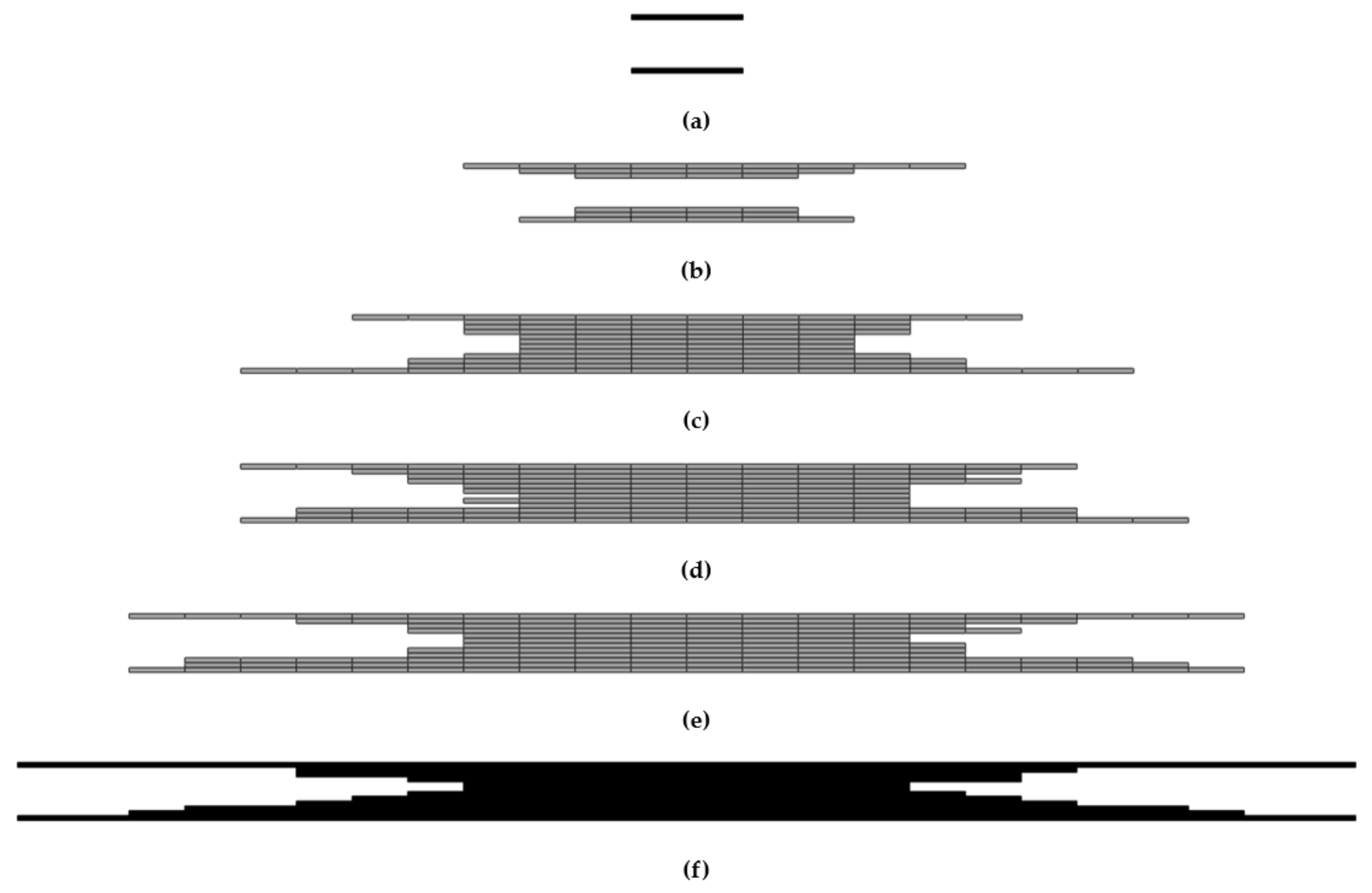
Figure 14.
The cross-section profile of the damaged area; 0.5 J (a); 1.0 J (b); 2.5 J (c); 5.0 J (d); 7.5 J (e); 10.0 J (f).
Figure 14.
The cross-section profile of the damaged area; 0.5 J (a); 1.0 J (b); 2.5 J (c); 5.0 J (d); 7.5 J (e); 10.0 J (f).
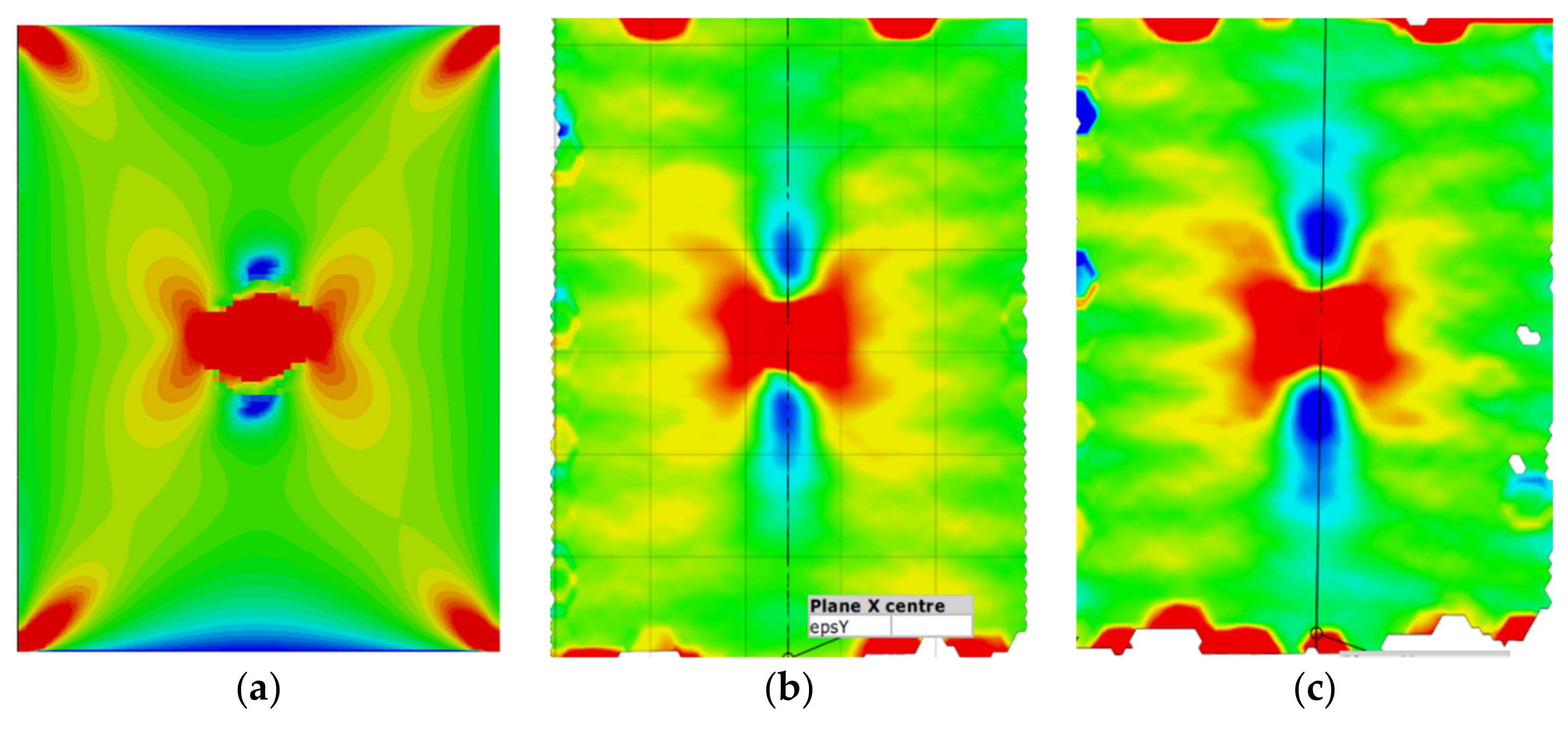
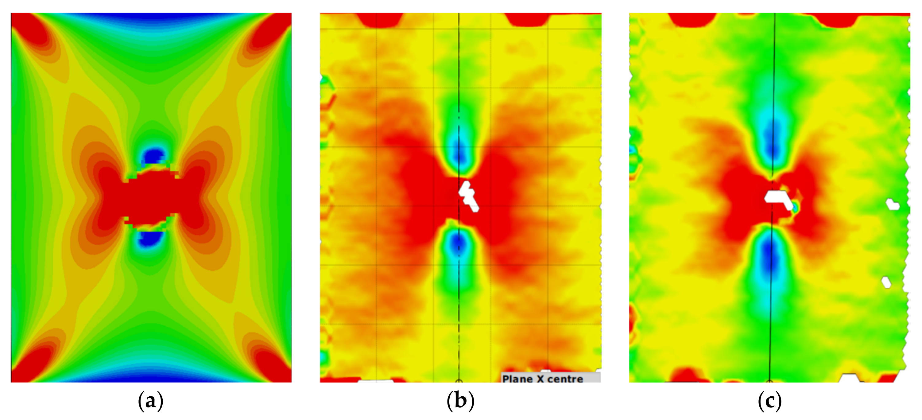
Figure 15.
Max. principal strain distribution (μm/m) at load 80 kN; (a) Simulation; (b) Experiment sample 1; (c) Experiment sample 2.
Figure 15.
Max. principal strain distribution (μm/m) at load 80 kN; (a) Simulation; (b) Experiment sample 1; (c) Experiment sample 2.
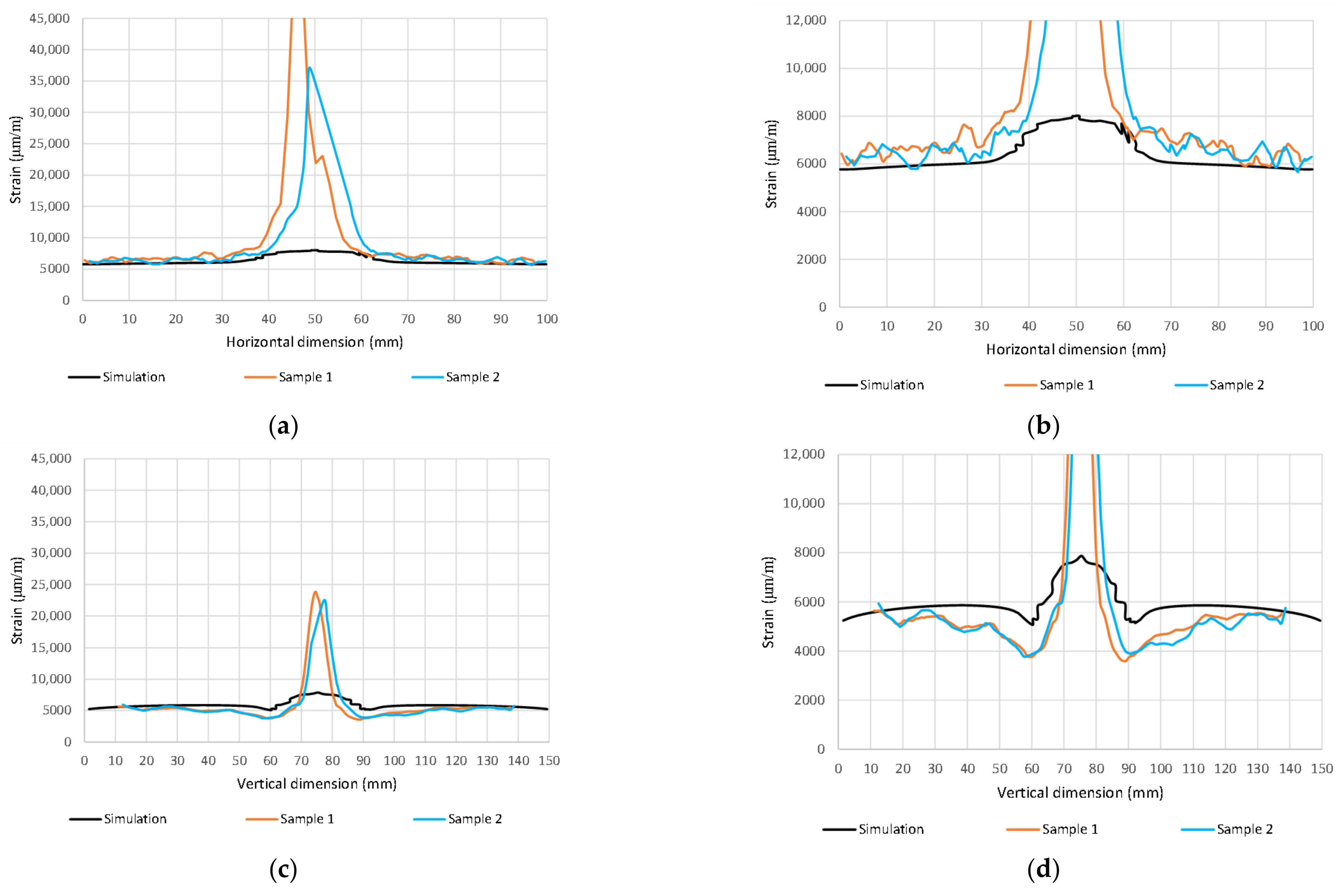
Figure 16.
Max. principal strain distribution (μm/m) at load 80 kN; (a) Horizontal path—scale 1; (b) Horizontal path—scale 2; (c) Vertical path—scale 1; (d) Vertical path—scale 2.
Figure 16.
Max. principal strain distribution (μm/m) at load 80 kN; (a) Horizontal path—scale 1; (b) Horizontal path—scale 2; (c) Vertical path—scale 1; (d) Vertical path—scale 2.
Figure 17.
Max. principal strain distribution (μm/m) at load 110 kN; (a) Simulation; (b) Experiment sample 1; (c) Experiment sample 2.
Figure 17.
Max. principal strain distribution (μm/m) at load 110 kN; (a) Simulation; (b) Experiment sample 1; (c) Experiment sample 2.
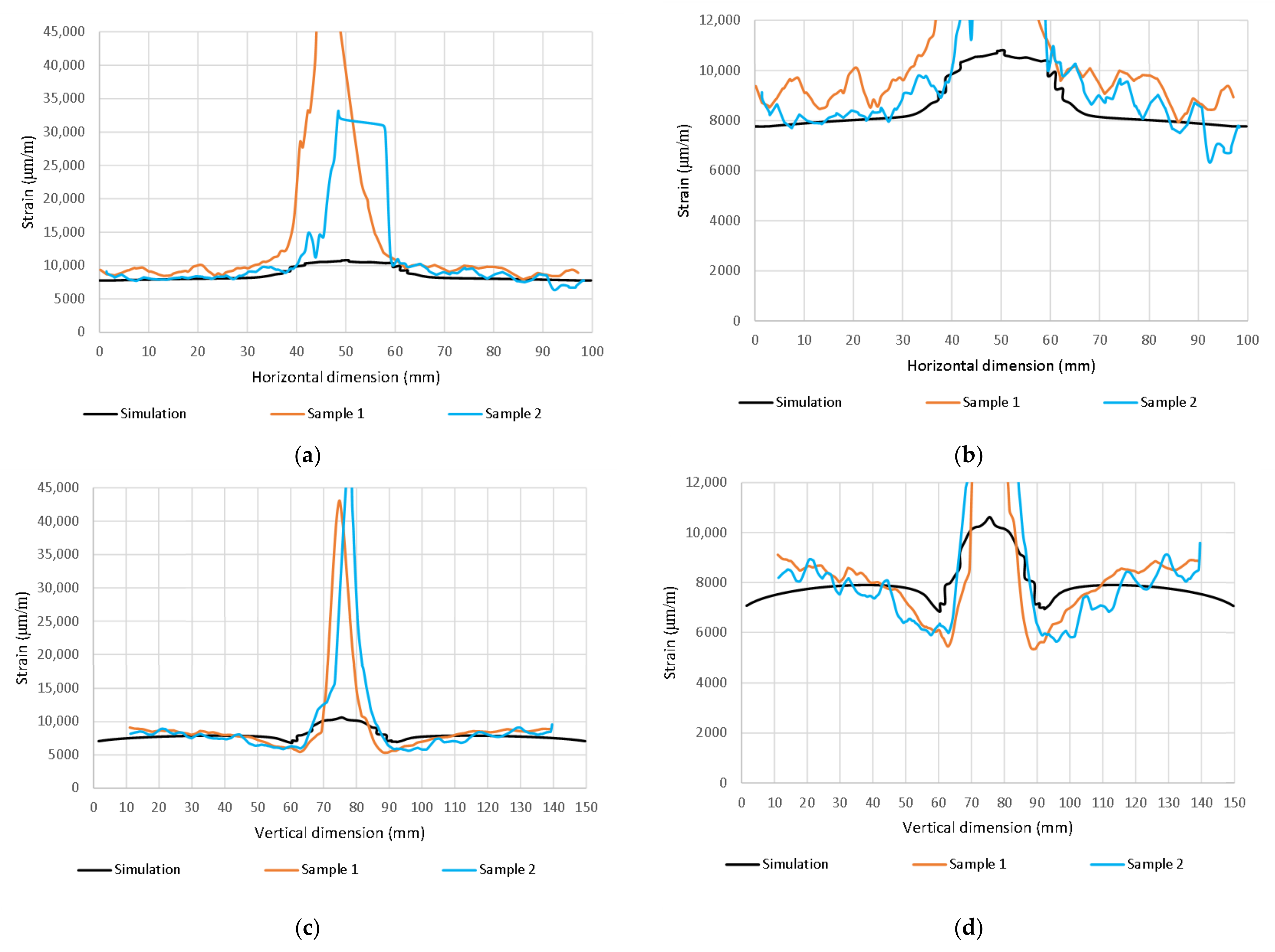
Figure 18.
Max. principal strain distribution (μm/m) at load 110 kN; (a) Horizontal path—scale 1; (b) Horizontal path—scale 2; (c) Vertical path—scale 1; (d) Vertical path—scale 2.
Figure 18.
Max. principal strain distribution (μm/m) at load 110 kN; (a) Horizontal path—scale 1; (b) Horizontal path—scale 2; (c) Vertical path—scale 1; (d) Vertical path—scale 2.
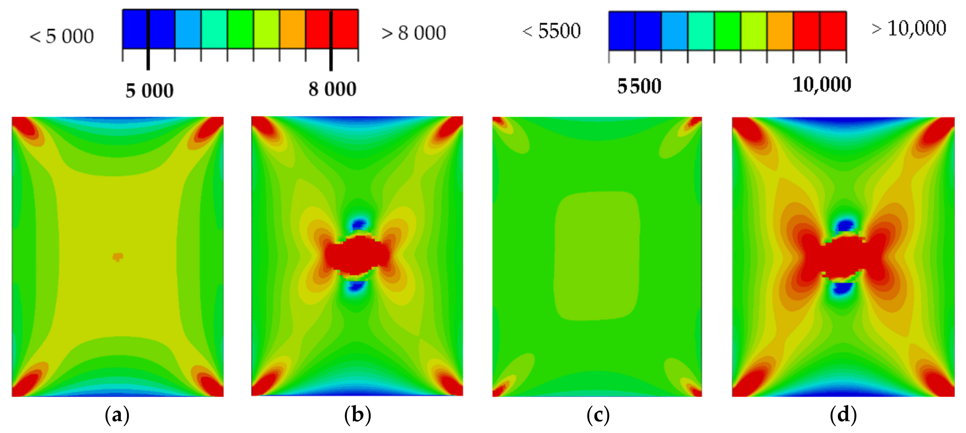
Figure 19.
Max. principal strain distribution (μm/m); Pristine 80 kN (a); Damaged (10 J) 80 kN (b); Pristine 110 kN (c); Damaged (10 J) 110 kN (d).
Figure 19.
Max. principal strain distribution (μm/m); Pristine 80 kN (a); Damaged (10 J) 80 kN (b); Pristine 110 kN (c); Damaged (10 J) 110 kN (d).
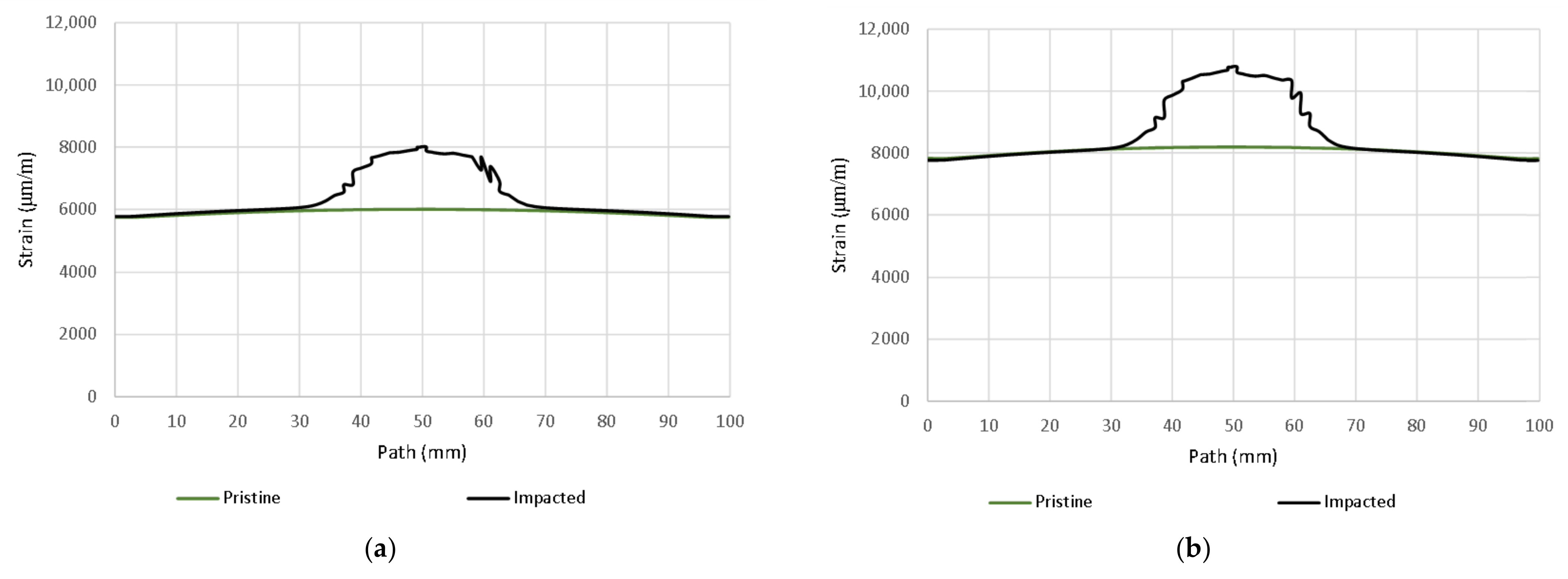
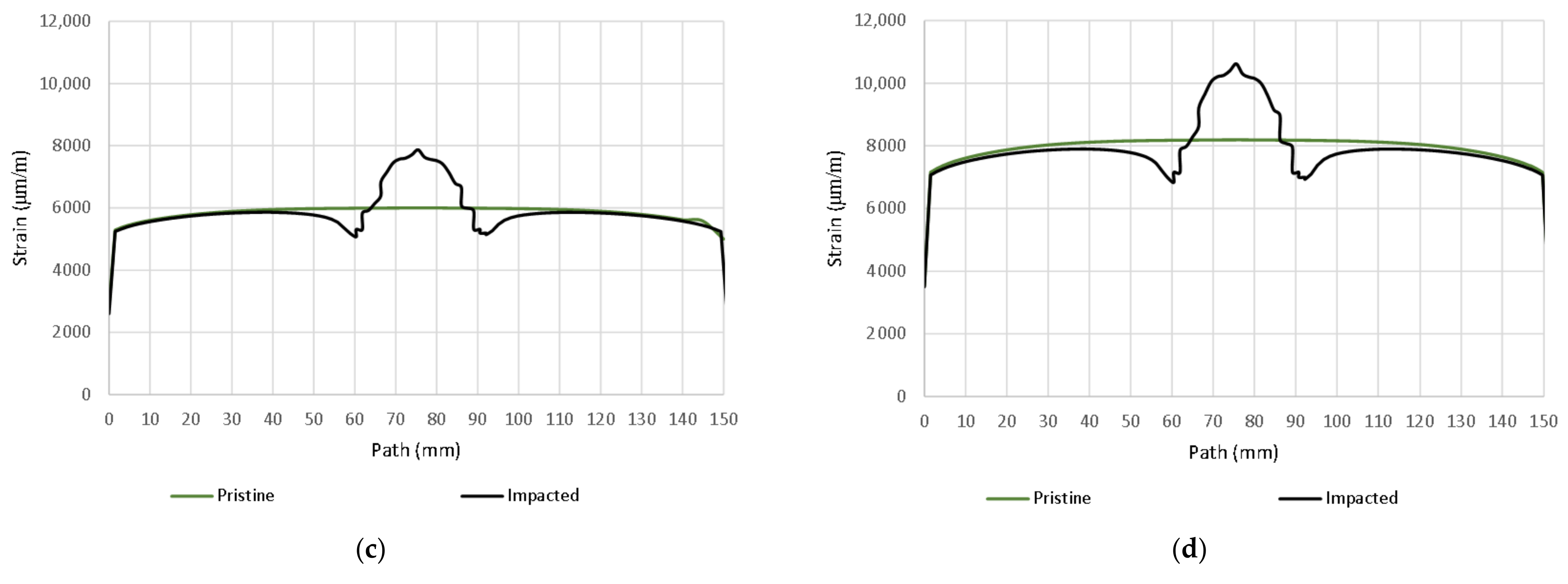
Figure 20.
Comparison of max. principal strain distribution (μm/m); (a) Horizontal path at load 80 kN; (b) Horizontal path at load 110 kN, (c) Vertical path at load 80 kN; (d) Vertical path at load 110 kN.
Figure 20.
Comparison of max. principal strain distribution (μm/m); (a) Horizontal path at load 80 kN; (b) Horizontal path at load 110 kN, (c) Vertical path at load 80 kN; (d) Vertical path at load 110 kN.
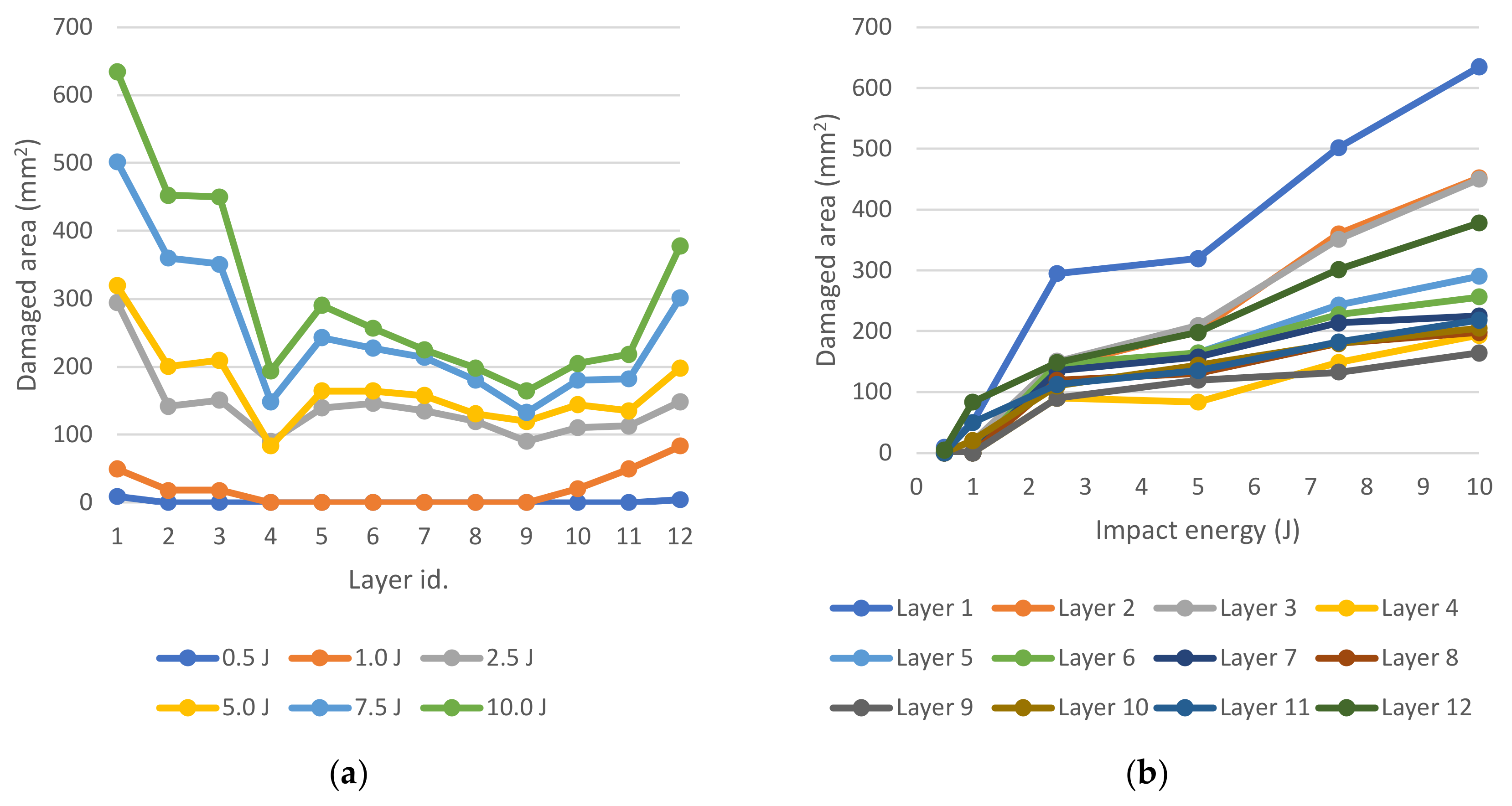
Figure 21.
Ply damage distribution; Damaged area vs. layer (a); Damaged area vs. impact energy (b).
Figure 21.
Ply damage distribution; Damaged area vs. layer (a); Damaged area vs. impact energy (b).
Table 1.
The elastic properties of the lamina.
Table 1.
The elastic properties of the lamina.
| | | | | |
|---|
| 129,840 | 13,340 | 0.26 | 4890 | 4890 | 4630 |
Table 2.
The strength of the lamina.
Table 2.
The strength of the lamina.
| | | | | |
|---|
| 2965.41 | 2911.81 | 100.88 | 109.42 | 100.76 | 98.41 |
Table 3.
The Hashin damage evolution parameters of the lamina.
Table 3.
The Hashin damage evolution parameters of the lamina.
| | | |
|---|
| 35.56 | 34.28 | 0.92 | 1.08 |
Table 4.
The strength parameters of cohesive contact.
Table 4.
The strength parameters of cohesive contact.
| | | |
|---|
| >45 | 100.88 | 100.76 | 100.76 |
| ≤45 | 174.03 | 173.44 | 173.44 |
Table 5.
The damage evolution parameters of cohesive contact.
Table 5.
The damage evolution parameters of cohesive contact.
| | |
|---|
| 35.56 | 0.92 | 0.92 |
Table 6.
Proper elastic properties of damaged lamina.
Table 6.
Proper elastic properties of damaged lamina.
| | | | | |
|---|
| | | | | |
Table 7.
Sample stiffness and strength check (0°).
Table 7.
Sample stiffness and strength check (0°).
| | Experiment | Simulation |
|---|
| Tensile modulus | 76,965 ± 863 MPa | 76,964 MPa |
| Poisson ratio | 0.30 ± 0.03 | 0.3 |
| Ultimate tensile load | 49,820 ± 1075 N | 50,854 N |
Table 8.
The penetration of the sample by impactor.
Table 8.
The penetration of the sample by impactor.
| | Experiment | Simulation |
|---|
| Energy | 10.45 ± 0.22 J | 10.45 J |
| Penetration | 6.99 ± 0.21 mm | 6.71 mm |
| Residual deformation | 1.12 ± 0.36 mm | 0.77 mm |


