
3D Polymer Architectures for the Identification of Optimal Dimensions for Cellular Growth of 3D Cellular Models

Abstract
:1. Introduction
2. Materials and Methods
2.1. Structure Design
2.2. Two-Photon Polymerization Setup, Sample Preparation and Characterization
Optical and SEM Imaging
2.3. Reduction of Polymer Auto-Fluorescence
2.4. Cell Culture and Staining of A549 Cells
2.5. Confocal Imaging
2.6. 3D Hyperspectral Image Analysis via Spectral Linear Unmixing
3. Results and Discussion
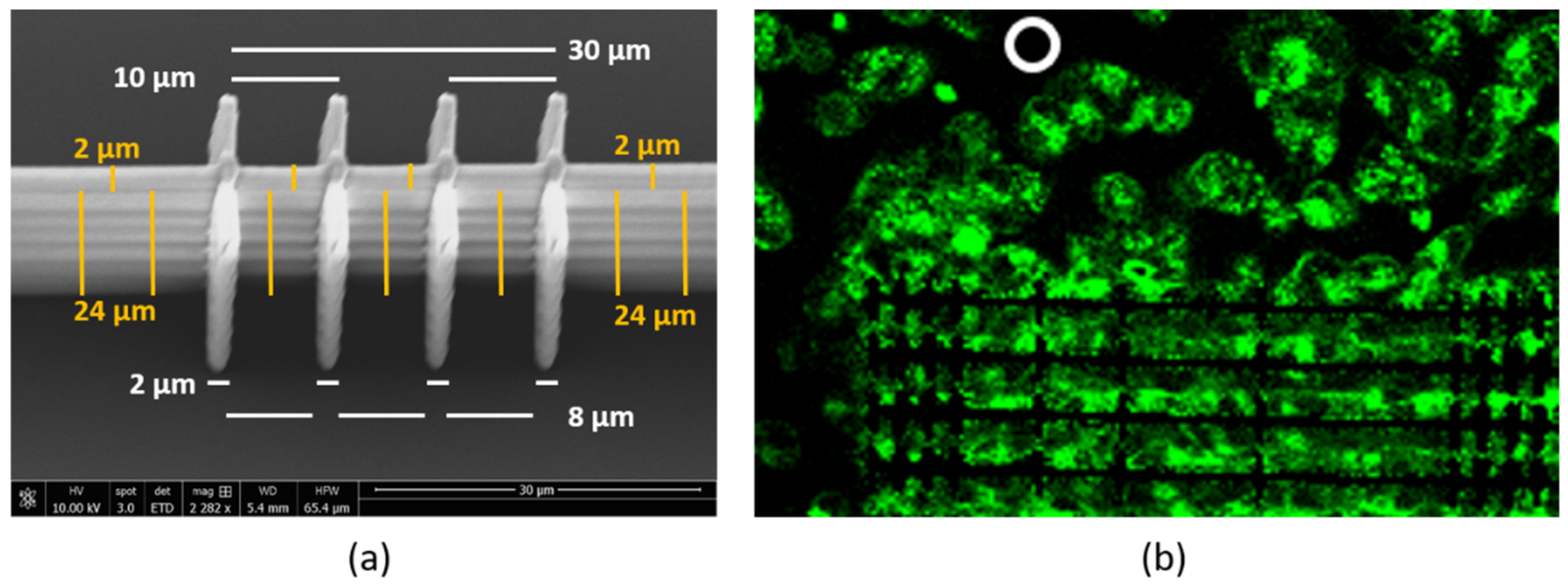
3.1. Development of 3D Scaffolds
3.2. Reduction of SZ2080 Polymer’s Auto-Fluorescence
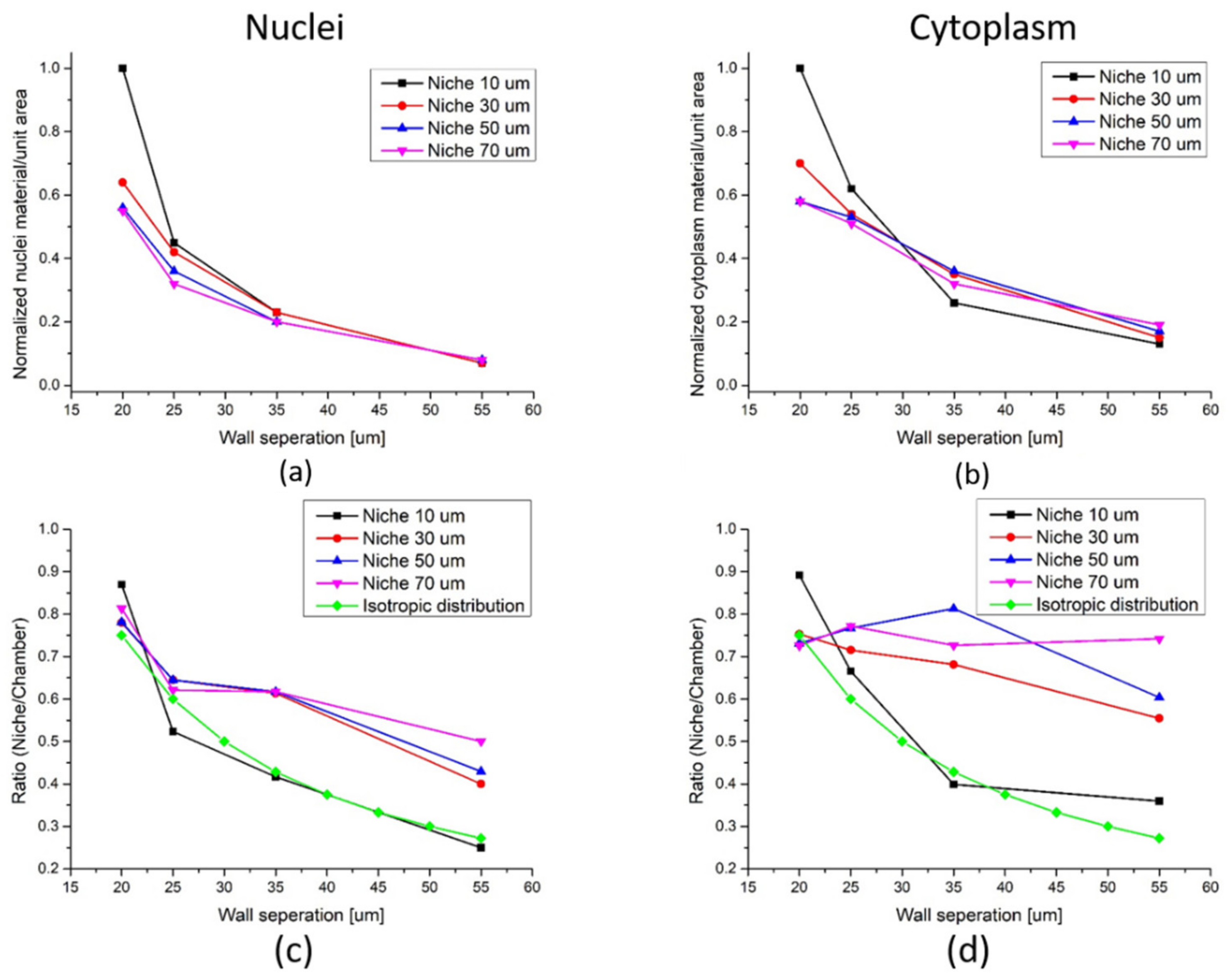
3.3. Analysis of Scaffold Influence on Cell Packing
3.4. Observation of 3D Cellular Vertical Growth over Time as a Function of Wall Separation
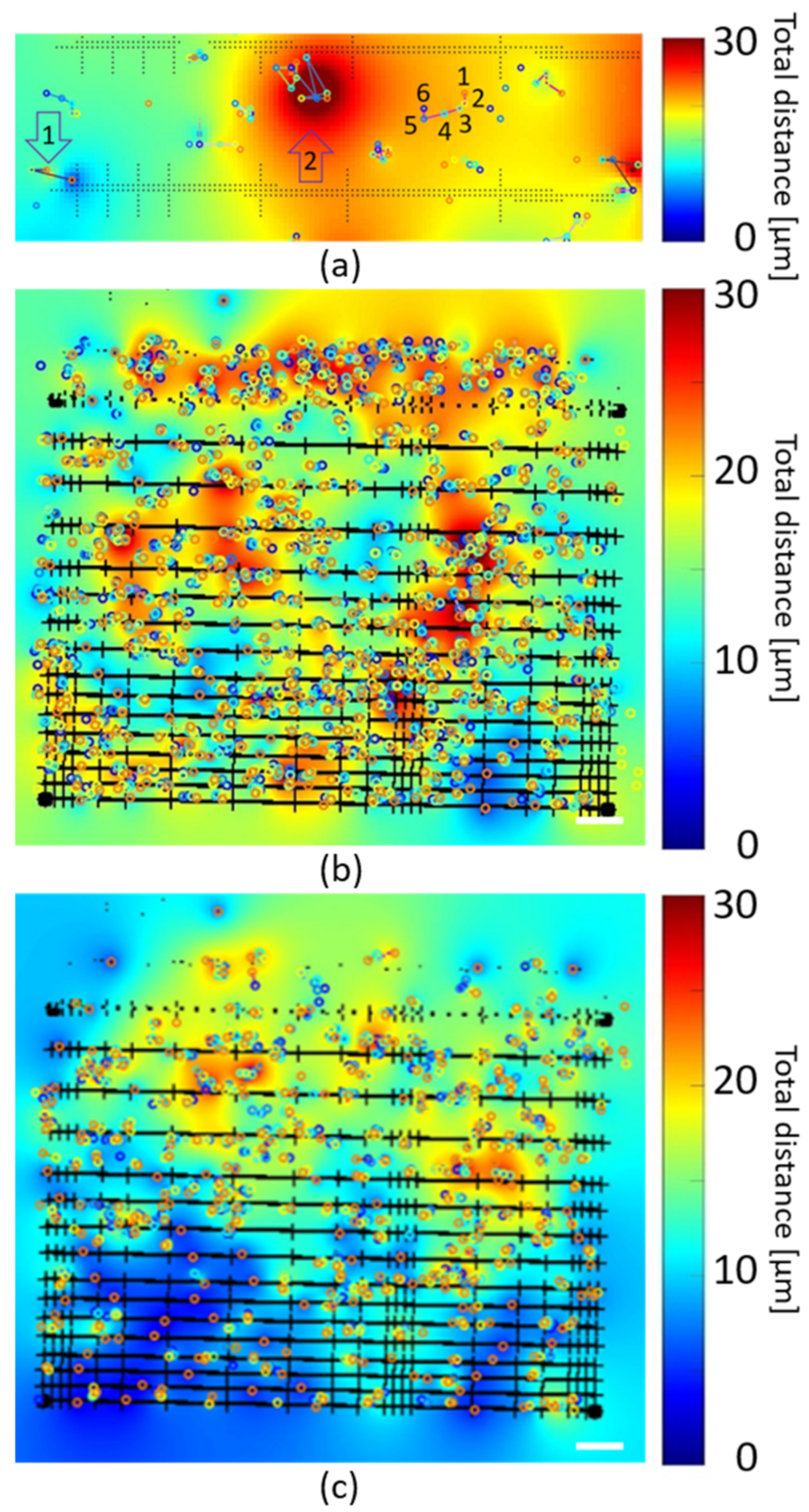
3.5. Analysis of Cell Movement Compared to Scaffold Wall Separation and Niche Size
4. Conclusions
Supplementary Materials
Author Contributions
Funding
Acknowledgments
Conflicts of Interest
Appendix A


| N [Pixels] | 2 | 5 | 7 | 10 | 12 | 15 |
|---|---|---|---|---|---|---|
| N [µm] | 3.32 | 8.3 | 11.62 | 16.6 | 19.92 | 24.9 |
| Interval [µm] | [0–19.92] | [0–49.8] | [0–69.72] | [0–99.6] | [0–119.52] | [0–149.4] |
| Max travel identified [µm] | 5 | 20 | 25 | 30 | 35 | 45 |
| Ratio [Interval/Max travel] | 4 | 2.49 | 2.788 | 3.32 | 3.44 | 3.32 |
| % of maximum allowed travel | 25 | 40 | 35 | 30 | 29 | 30 |


References
- Low, L.A.; Mummery, C.; Berridge, B.R.; Austin, C.P.; Tagle, D.A. Organs-on-chips: Into the next decade. Nat. Rev. Drug Discov. 2021, 20, 345–361. [Google Scholar] [CrossRef] [PubMed]
- Wu, Q.; Liu, J.; Wang, X.; Feng, L.; Wu, J.; Zhu, X.; Wen, W.; Gong, X. Organ-on-a-chip: Recent breakthroughs and future prospects. Biomed. Eng. Online 2020, 19, 9. [Google Scholar] [CrossRef] [PubMed] [Green Version]
- Esch, E.W.; Bahinski, A.; Huh, D. Organs-on-chips at the frontiers of drug discovery. Nat. Rev. Drug Discov. 2015, 14, 248–260. [Google Scholar] [CrossRef] [PubMed] [Green Version]
- Trappmann, B.; Baker, B.M.; Polacheck, W.J.; Choi, C.K.; Burdick, J.A.; Chen, C.S. Matrix degradability controls multicellularity of 3D cell migration. Nat. Commun. 2017, 8, 371. [Google Scholar] [CrossRef] [Green Version]
- Safaee, H.; Bakooshli, M.A.; Davoudi, S.; Cheng, R.Y.; Martowirogo, A.J.; Li, E.W.; Simmons, C.A.; Gilbert, P.M. Tethered Jagged-1 Synergizes with Culture Substrate Stiffness to Modulate Notch-Induced Myogenic Progenitor Differentiation. Cell. Mol. Bioeng. 2017, 10, 501–513. [Google Scholar] [CrossRef]
- Rudmann, D.G. The Emergence of Microphysiological Systems (Organs-on-chips) as Paradigm-changing Tools for Toxicologic Pathology. Toxicol. Pathol. 2018, 47, 4–10. [Google Scholar] [CrossRef]
- Cao, X.; Coyle, J.P.; Xiong, R.; Wang, Y.; Heflich, R.H.; Ren, B.; Gwinn, W.M.; Hayden, P.; Rojanasakul, L. Invited review: Human air-liquid-interface organotypic airway tissue models derived from primary tracheobronchial epithelial cells—Overview and perspectives. Vitr. Cell. Dev. Biol.-Anim. 2020, 57, 104–132. [Google Scholar] [CrossRef]
- Hiemstra, P.S.; Grootaers, G.; van der Does, A.M.; Krul, C.A.M.; Kooter, I.M. Human lung epithelial cell cultures for analysis of inhaled toxicants: Lessons learned and future directions. Toxicol. Vitr. 2018, 47, 137–146. [Google Scholar] [CrossRef]
- Huh, D.; Matthews, B.D.; Mammoto, A.; Montoya-Zavala, M.; Yuan Hsin, H.; Ingber, D.E. Reconstituting organ-level lung functions on a chip. Science 2010, 328, 1662–1668. [Google Scholar] [CrossRef] [Green Version]
- Baptista, D.; Teixeira, L.M.; Birgani, Z.T.; van Riet, S.; Pasman, T.; Poot, A.; Stamatialis, D.; Rottier, R.J.; Hiemstra, P.S.; Habibović, P.; et al. 3D alveolar in vitro model based on epithelialized biomimetically curved culture membranes. Biomaterials 2021, 266, 120436. [Google Scholar] [CrossRef]
- Moinuddin, M.G.; Kumar, R.; Yogesh, M.; Sharma, S.; Sahani, M.; Sharma, S.K.; Gonsalves, K.E. Functionalized Ag Nanoparticles Embedded in Polymer Resists for High-Resolution Lithography. ACS Appl. Nano Mater. 2020, 3, 8651–8661. [Google Scholar] [CrossRef]
- Zhu, J.; Chen, Y.; Xie, S.; Zhang, L.; Wang, C.; Tai, R. Nanofabrication of 30 nm Au zone plates by e-beam lithography and pulse voltage electroplating for soft x-ray imaging. Microelectron. Eng. 2020, 225, 111254. [Google Scholar] [CrossRef]
- Lemma, E.D.; Sergio, S.; Spagnolo, B.; Pisanello, M.; Algieri, L.; Coluccia, M.A.; Maffia, M.; De Vittorio, M.; Pisanello, F. Tunable mechanical properties of stent-like microscaffolds for studying cancer cell recognition of stiffness gradients. Microelectron. Eng. 2018, 190, 11–18. [Google Scholar] [CrossRef]
- Spagnolo, B.; Brunetti, V.; Leménager, G.; De Luca, E.; Sileo, L.; Pellegrino, T.; Paolo Pompa, P.; De Vittorio, M.; Pisanello, F. Three-dimensional cage-like microscaffolds for cell invasion studies. Sci. Rep. 2015, 5, 10531. [Google Scholar] [CrossRef] [Green Version]
- Saha, S.K.; Wang, D.; Nguyen, V.H.; Chang, Y.; Oakdale, J.S.; Chen, S.C. Scalable submicrometer additive manufacturing. Science 2019, 366, 105–109. [Google Scholar] [CrossRef]
- Zhu, W.; Ma, X.; Gou, M.; Mei, D.; Zhang, K.; Chen, S. 3D printing of functional biomaterials for tissue engineering. Curr. Opin. Biotechnol. 2016, 40, 103–112. [Google Scholar] [CrossRef] [Green Version]
- Mačiulaitis, J.; Deveikytė, M.; Rekštytė, S.; Bratchikov, M.; Darinskas, A.; Šimbelytė, A.; Daunoras, G.; Laurinavičienė, A.; Laurinavičius, A.; Gudas, R.; et al. Preclinical study of SZ2080 material 3D microstructured scaffolds for cartilage tissue engineering made by femtosecond direct laser writing lithography. Biofabrication 2015, 7, 15015. [Google Scholar] [CrossRef]
- Tammaro, D.; Della Gatta, R.; Villone, M.M.; Maffettone, P.L. Continuous 3D Printing of Hierarchically Structured Microfoamed Objects. Adv. Eng. Mater. 2022, 24, 2101226. [Google Scholar] [CrossRef]
- Khalaf, A.T.; Wei, Y.; Wan, J.; Zhu, J.; Peng, Y.; Abdul Kadir, S.Y.; Zainol, J.; Oglah, Z.; Cheng, L.; Shi, Z. Bone Tissue Engineering through 3D Bioprinting of Bioceramic Scaffolds: A Review and Update. Life 2022, 12, 903. [Google Scholar] [CrossRef]
- Su, Y.; Toftdal, M.S.; Le Friec, A.; Dong, M.; Han, X.; Chen, M. 3D Electrospun Synthetic Extracellular Matrix for Tissue Regeneration. Small Sci. 2021, 1, 2100003. [Google Scholar] [CrossRef]
- Skliutas, E.; Lebedevaite, M.; Kabouraki, E.; Baldacchini, T.; Ostrauskaite, J.; Vamvakaki, M.; Farsari, M.; Juodkazis, S.; Malinauskas, M. Photopolymerization Mechanisms at a Spatio-Temporally Ultra-Confined Light; De Gruyter: Berlin, Germany, 2020. [Google Scholar]
- Costa, B.N.L.; Adão, R.M.R.; Maibohm, C.; Accardo, A.; Cardoso, V.F.; Nieder, J.B. Cellular Interaction of Bone Marrow Mesenchymal Stem Cells with Polymer and Hydrogel 3D Microscaffold Templates. ACS Appl. Mater. Interfaces 2022, 14, 13013–13024. [Google Scholar] [CrossRef]
- Maibohm, C.; Saldana-Lopez, A.; Silvestre, O.F.; Nieder, J.B. 3D Polymer Structures for the Identification of Optimal Dimensions for Cellular Growth for 3D Lung Alveolar Models. Eng. Proc. 2021, 4, 33. [Google Scholar] [CrossRef]
- Jiang, R.D.; Shen, H.; Piao, Y.J. The morphometrical analysis on the ultrastructure of a549 cells. Rom. J. Morphol. Embryol. 2010, 51, 663–667. [Google Scholar]
- Maibohm, C.; Silvestre, O.F.; Borme, J.; Sinou, M.; Heggarty, K.; Nieder, J.B. Multi-beam two-photon polymerization for fast large area 3D periodic structure fabrication for bioapplications. Sci. Rep. 2020, 10, 8740. [Google Scholar] [CrossRef]
- Ovsianikov, A.; Viertl, J.; Chichkov, B.; Oubaha, M.; MacCraith, B.; Sakellari, I.; Giakoumaki, A.; Gray, D.; Vamvakaki, M.; Farsari, M.; et al. Ultra-low shrinkage hybrid photosensitive material for two-photon polymerization microfabrication. ACS Nano 2008, 2, 2257–2262. [Google Scholar] [CrossRef]
- Flamourakis, G.; Kordas, A.; Barmparis, G.D.; Ranella, A.; Farsari, M. Low-autofluorescence, transparent composite for multiphoton 3D printing. Opt. Mater. Express 2021, 11, 801–813. [Google Scholar] [CrossRef]
- Qi, L.; Knapton, E.K.; Zhang, X.; Zhang, T.; Gu, C.; Zhao, Y. Pre-culture Sudan Black B treatment suppresses autofluorescence signals emitted from polymer tissue scaffolds. Sci. Rep. 2017, 7, 8361. [Google Scholar] [CrossRef] [Green Version]
- Kauanova, S.; Urazbayev, A.; Vorobjev, I. The Frequent Sampling of Wound Scratch Assay Reveals the “Opportunity” Window for Quantitative Evaluation of Cell Motility-Impeding Drugs. Front. Cell Dev. Biol. 2021, 9, 640972. [Google Scholar] [CrossRef]
- Ebrahimi, Z.; Irani, S.; Ardeshirylajimi, A.; Seyedjafari, E. Enhanced osteogenic differentiation of stem cells by 3D printed PCL scaffolds coated with collagen and hydroxyapatite. Sci. Rep. 2022, 12, 12359. [Google Scholar] [CrossRef]
- Scarian, E.; Bordoni, M.; Fantini, V.; Jacchetti, E.; Raimondi, M.T.; Diamanti, L.; Carelli, S.; Cereda, C.; Pansarasa, O. Patients’ Stem Cells Differentiation in a 3D Environment as a Promising Experimental Tool for the Study of Amyotrophic Lateral Sclerosis. Int. J. Mol. Sci. 2022, 23, 5344. [Google Scholar] [CrossRef]
- Zhao, X.; Li, Q.; Guo, Z.; Li, Z. Constructing a cell microenvironment with biomaterial scaffolds for stem cell therapy. Stem Cell Res. Ther. 2021, 12, 583. [Google Scholar] [CrossRef] [PubMed]
- Nicolas, J.; Magli, S.; Rabbachin, L.; Sampaolesi, S.; Nicotra, F.; Russo, L. 3D Extracellular Matrix Mimics: Fundamental Concepts and Role of Materials Chemistry to Influence Stem Cell Fate. Biomacromolecules 2020, 21, 1968–1994. [Google Scholar] [CrossRef] [PubMed]
- Akolawala, Q.; Rovituso, M.; Versteeg, H.H.; Rondon, A.M.R.; Accardo, A. Evaluation of Proton-Induced DNA Damage in 3D-Engineered Glioblastoma Microenvironments. ACS Appl. Mater. Interfaces 2022, 14, 20778–20789. [Google Scholar] [CrossRef] [PubMed]
- Maibohm, C.; Silva, F.; Figueiras, E.; Guerreiro, P.T.; Brito, M.; Romero, R.; Crespo, H.; Nieder, J.B. SyncRGB-FLIM: Synchronous fluorescence imaging of red, green and blue dyes enabled by ultra-broadband few-cycle laser excitation and fluorescence lifetime detection. Biomed. Opt. Express 2019, 10, 1891–1904. [Google Scholar] [CrossRef]
- Faria, A.R.; Silvestre, O.F.; Maibohm, C.; Adão, R.M.R.; Silva, B.F.B.; Nieder, J.B. Cubosome nanoparticles for enhanced delivery of mitochondria anticancer drug elesclomol and therapeutic monitoring via sub-cellular NAD(P)H multi-photon fluorescence lifetime imaging. Nano Res. 2019, 12, 991–998. [Google Scholar] [CrossRef]
- Rabbi, F.; Dabbagh, S.R.; Angin, P.; Yetisen, A.K.; Tasoglu, S. Deep Learning-Enabled Technologies for Bioimage Analysis. Micromachines 2022, 13, 260. [Google Scholar] [CrossRef]
- Joy, D.A.; Libby, A.R.G.; McDevitt, T.C. Deep neural net tracking of human pluripotent stem cells reveals intrinsic behaviors directing morphogenesis. Stem Cell Rep. 2021, 16, 1317–1330. [Google Scholar] [CrossRef]


| Wall Separation | Bottom (Figure 7b) | Top (Figure 7b) | Figure 6c |
|---|---|---|---|
| 20 µm | [0.84–0.97] | [0.73–1.00] | [0.78–0.86] |
| 25 µm | [0.76–0.85] | [0.76–0.94] | [0.52–0.64] |
| 35 µm | [0.74–0.88] | [0.59–0.73] | [0.41–0.62] |
| 55 µm | [0.46–0.56] | [0.50–0.58] | [0.25–0.50] |
Publisher’s Note: MDPI stays neutral with regard to jurisdictional claims in published maps and institutional affiliations. |
© 2022 by the authors. Licensee MDPI, Basel, Switzerland. This article is an open access article distributed under the terms and conditions of the Creative Commons Attribution (CC BY) license (https://creativecommons.org/licenses/by/4.0/).
Share and Cite
Maibohm, C.; Saldana-Lopez, A.; Silvestre, O.F.; Nieder, J.B. 3D Polymer Architectures for the Identification of Optimal Dimensions for Cellular Growth of 3D Cellular Models. Polymers 2022, 14, 4168. https://doi.org/10.3390/polym14194168
Maibohm C, Saldana-Lopez A, Silvestre OF, Nieder JB. 3D Polymer Architectures for the Identification of Optimal Dimensions for Cellular Growth of 3D Cellular Models. Polymers. 2022; 14(19):4168. https://doi.org/10.3390/polym14194168
Chicago/Turabian StyleMaibohm, Christian, Alberto Saldana-Lopez, Oscar F. Silvestre, and Jana B. Nieder. 2022. "3D Polymer Architectures for the Identification of Optimal Dimensions for Cellular Growth of 3D Cellular Models" Polymers 14, no. 19: 4168. https://doi.org/10.3390/polym14194168