Article

Effects of Input Parameter Range on the Accuracy of Artificial Neural Network Prediction for the Injection Molding Process

1
Department of Mechanical Engineering, Dankook University, Yongin 16890, Korea
2
Molding & Metal Forming R&D Department, Korea Institute of Industrial Technology, Bucheon 14442, Korea
3
SimTech, Bucheon 14442, Korea
*
Authors to whom correspondence should be addressed.
Polymers 2022, 14(9), 1724; https://doi.org/10.3390/polym14091724
Submission received: 14 March 2022 / Revised: 15 April 2022 / Accepted: 21 April 2022 / Published: 23 April 2022
(This article belongs to the Special Issue Advances in Polymers Processing and Injection Molding)

Abstract

:
Artificial neural network (ANN) is a representative technique for identifying relationships that contain complex nonlinearities. However, few studies have analyzed the ANN’s ability to represent nonlinear or linear relationships between input and output parameters in injection molding. The melt temperature, mold temperature, injection speed, packing pressure, packing time, and cooling time were chosen as input parameters, and the mass, diameter, and height of the injection molded product as output parameters to construct an ANN model and its prediction performance was compared with those of linear regression and second-order polynomial regression. Following the preliminary experiment results, the learning data sets were divided into two groups, i.e., one showed linear relation between the mass of the final product and the range of packing time (linear relation group), and the other showed clear nonlinear relation (nonlinear relation group). The predicted results of ANN were relatively better than those of linear regression and second-order polynomial for both linear and nonlinear relation groups in our specific data sets of the present study.

1. Introduction

Injection molding is a representative plastic molding technique that can rapidly produce products with complex shapes, which require precise dimensions, in large batches. This technique is widely used in various fields, ranging from household goods to the automotive industry or electronic and electrical industries [1,2]. It is the process of molding a product by injecting a plastic resin melted at a high temperature into a space with a specific shape within a mold at high speed and pressure. Thus, the rheological behavior and state of the material during molding are affected by input process conditions, i.e., the melt and mold temperatures, injection speed, packing pressure, and packing time. Those five variables ultimately affect the final product quality, i.e., mass or dimensions of the final product. The fabrication of a product with the desired quality requires specific combinations of input process conditions. If the input process conditions are unsuitable, defects such as short shots or flash may occur. However, because the plastics used in the injection molding process have highly complex thermo-viscoelastic behavior, it is difficult to realize and maintain the desired quality [3]. In production sites where the injection molding process is applied, a trial-and-error approach has been frequently used to explore process conditions through references or guidebooks. It requires significant time and cost, as well as involving high uncertainty because it depends heavily on the experience of molding workers. To resolve these issues, the computer aided engineering (CAE) technique has been applied as a very useful pretest tool that can model the relationship between injection molding parameters and final quality and optimize the process [4,5,6]. However, the injection molding simulation analysis utilizing the CAE consumes significant time when estimating the final dimensions, in addition to the many assumptions concerning the material properties [3]. Furthermore, despite the increased accuracy of recent CAE analysis, it is well known that there have been differences between the predicted and actual values of output quality due to the inherent nonlinear and viscoelastic characteristics of plastic resins.
Thus, there has been a consistent need for a new and improved method for optimally manufacturing injection molded products with a targeted output, such as mass or specific lengths. In response to this demand, there has recently been an increasing amount of research applying artificial neural network (ANN) technology to model and optimize the relationship between input variables, such as melt and mold temperatures, and output variables, such as mass or specific length in the injection molding process [7,8,9,10,11,12,13,14,15,16]. The ANN, currently the most promising language in the artificial intelligence (AI) field, is a well-known and representative technique exhibiting powerful and practical performance in identifying relationships that contain complex nonlinearities [3]. Ozcelik et al. [7] constructed an ANN with a multi-input single-output (MISO) structure, in which five multi-input parameters, i.e., melt temperature, mold temperature, packing pressure and time, and cooling time, were set to perform an injection molding experiment. The warpage of a molded product was measured at a specific location, which was chosen as the targeted output (single output). They conducted and demonstrated the usefulness of the MISO structure to predict the molding conditions for minimizing the amount of warpage at specific locations. Yin et al. [8] set the same five input parameters and obtained the warpage information of the automobile glove compartment cap through CAE results data rather than actual experiments. Similar to Ozcelik et al. [7], they constructed an ANN by applying the MISO structure and verified whether the amount of warpage was the minimum through actual experimentation by predicting the process conditions that minimize warpage. Yang et al. [9] set 10 process conditions as input parameters and built an ANN structure that predicts the mass of the injection molded product as an output parameter with MISO. They also conducted a study to determine the optimal set of process conditions for molding a product with a targeted mass. Their prediction showed good results while the relationships between input and output parameters were almost linear. Lee et al. [10] applied shape information such as volume and area for multiple molds in addition to the usual six process conditions as input parameters to predict the mass of a product for an arbitrary mold. The ANN was built by using experimental data and CAE analysis data. Based on the ANN model, they obtained good results by building a system for deriving the combination of input parameters that can be applied to molds of arbitrary shapes. Gim et al. [11] measured the cavity pressure and time using sensors. Then, five specific points, i.e., start point of filling stage, switchover point, maximum point of cavity pressure, packing endpoint, and cooling endpoint, were selected to extract pressure and time values and used as input parameters. ANN structure that predicts the mass of the injection molded product (spiral) as an output parameter with MISO. In addition, they conducted research on optimizing the molding window through sensitive analysis and obtained good results. Recently, as in the studies of Abdull et al. [12] and Heinisch et al. [13], research on multi-input multi-output (MIMO) structured ANNs is being actively performed to predict multiple target qualities from multiple process conditions. Table 1 lists studies in which ANNs are applied to the injection molding process.
In Table 1, previous studies used various shapes ranging from simple to complex, such as automobile glove components or IC trays. It can be seen that the injection molding process shows good results by using a simple ANN model, even with a complex shape or data structure. However, the linear range was applied in the relationship between parameters on a case-by-case basis, and this may suggest the possibility that limited results were obtained. In addition, it can be confirmed that most of the previous injection molding studies applied by ANNs are relatively simple structures, including one or two hidden layers or a small number of neurons. Concerning the nonlinearities, the performance of the ANN model is closely related to the complexity of the model [18]. In general, as the complexity increases, the number of hidden layers and neurons increases. The more nonlinear and complex the relationship between input and output parameters expressed in the ANN is, the greater the complexity required for the ANN model, and the problem may not be solved with a small number of hidden layers and neurons. Thus, when the number of hidden layers or neurons of the constructed ANN model is small, it can be considered a simple physical system with relatively strong linearity in the relationship between input and output parameters. Gim et al. [11], Abdul et al. [12], Heinisch et al. [13], Ke et al. [14], and Yang et al. [17] used an ANN model with one hidden layer for analyzing their specific data, while Ozcelik et al. [7], Yin et al. [8], Yang et al. [9], Lee et al. [10] and Huang et al. [15] used a model with two hidden layers. This means that the relationship between input and output parameters in the injection molding process can exhibit strong linearity. It can be possible to derive better results through other regression methods such as linear or polynomial. Therefore, to apply artificial neural networks to the injection molding process, it is necessary to check and exclude these possibilities. However, in previous studies on injection molding, confirmation and understanding of these problems were insufficient. In this respect, there have been studies comparing the performance of ANN with other regression analyses in the injection molding process. Heinisch et al. [13] set different methods for generating injection molding data groups and built ANN and Polynomial models to compare performance. After comparing the ANN and polynomial models, Heinisch et al. [13] concluded that they could not generally provide a guide regarding which method is better. These results are judged as the result of failing to represent the characteristics of each model by comparing the ANN and regression models only in the range where the relationship between parameters is linear.
Thus, preliminary experiments were performed to distinguish the data sets into linear and nonlinear groups. The range of packing time was chosen as an input parameter to determine the nonlinearity with the mass of the final product, a representative output parameter in preliminary experiments. In the data set of linear relation groups, the range of packing time was selected as 3.0~18.0 s, and the range of packing time was chosen as 3.0~30.0 s, including the packing time over 18.0 s for the data set of nonlinear relation group in the present study. Finally, in ANN modeling, linear and polynomial regressions were used for both linear and nonlinear groups to evaluate their respective accuracies and describe the strengths and weaknesses of each model.

2. Experiment

2.1. Material and Molding Equipment

In the present study, children’s tableware was selected as a target product, and a series of experiments were performed to obtain injection molding data. The target product was a bowl shape with a nominal diameter of 99.90 mm and a height of 50.80 mm, as shown in Figure 1a, and a two-stage mold with one cavity was utilized, as shown in Figure 1b. The hot runner system was applied to the mold, which is a direct system allowing the hot runner nozzle to be in contact with the center of the product. Polypropylene (PP) of LUPOL GP1007F (LG chemical) was used as the resin for product molding. The physical properties of LUPOL GP1007F described by the manufacturer are shown in Table 2. The 150-ton injection molding machine (LGEII-150, LSMtron) was used for the injection molding experiment. Table 3 shows the specifications of this injection molding machine.

2.2. Experimental Conditions

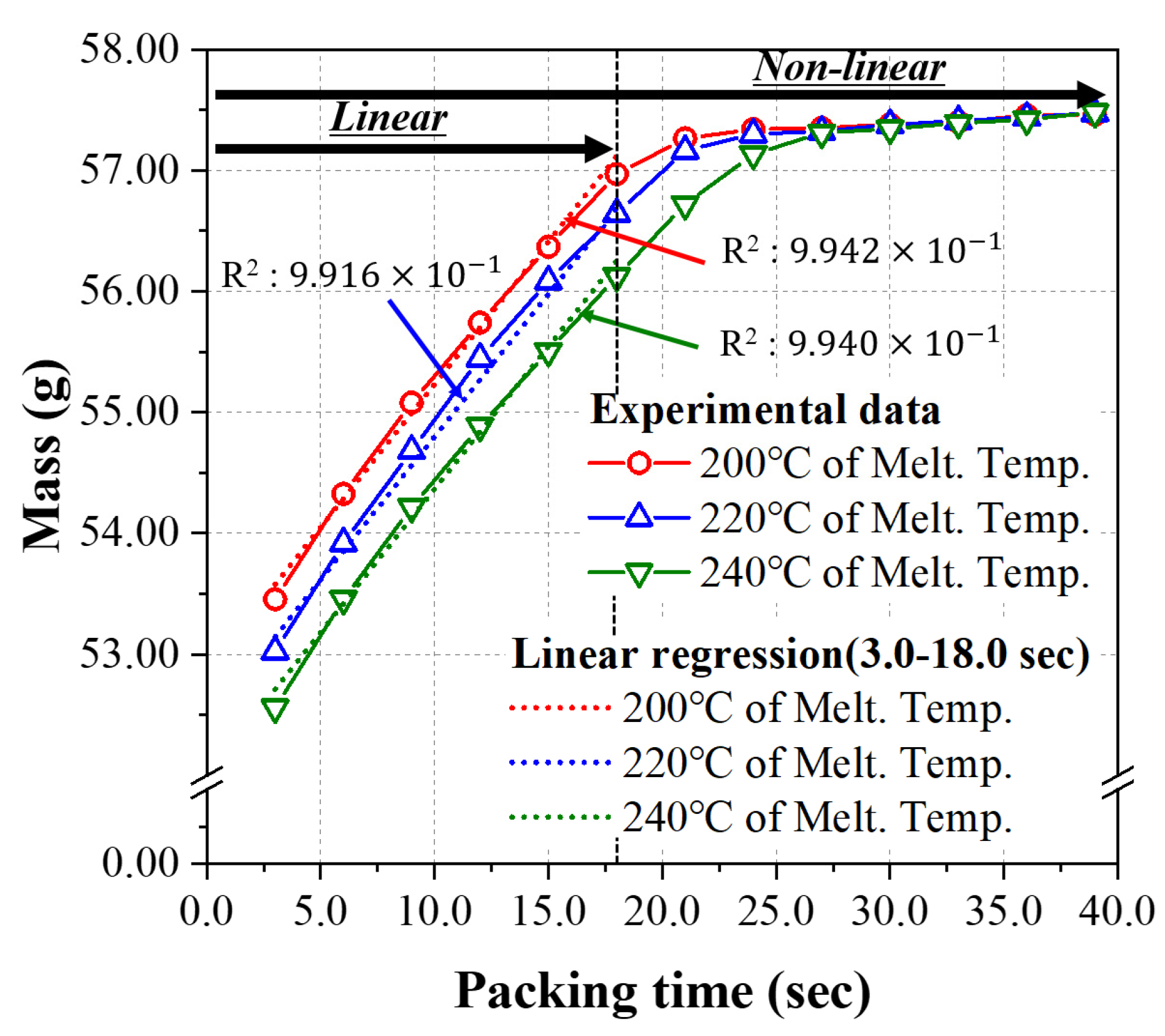
Based on the recommended conditions provided by the resin manufacturer and the database of Moldflow Insight 2021 (Autodesk), the melt temperature and mold temperature ranges were set in three levels for the injection molding experiment, as shown in Table 4. Furthermore, a series of preliminary experiments were performed to determine the process window of packing pressure and the range of packing time through which a normal product can be molded for the mold and product used in this study, and these were also applied in three levels. From the results of preliminary experiments, the performance of the ANN based on two groups of data sets was evaluated in the present study. The first group of data sets showed a strong linear relationship with an R2 score higher than 0.99 between the range of packing time (input parameter) and the mass of the molded product (output parameter). The second group of data sets showed a representative nonlinear relationship between them, as shown in Figure 2. The packing time of 6.0 s~18.0 s was applied to the data set of the linear relation group, as shown in Table 3, while the packing time of 3.0 s~39.0 s, including over 18.0 s, was applied to the data set of nonlinear relation group which will be shown in Table 5 later. The injection speed and cooling time were derived through CAE analysis using Moldflow Insight 2021, and the ranges of those process conditions were set at three levels, as are other conditions.
Table 5 lists 50 process conditions of above mentioned “linear relation group”. Based on the levels presented in Table 3, 27 combinations (experiment #1~#27) were created by the orthogonal array of L27, and 23 combinations (experiment #28~#50) were randomly generated within the corresponding range.
Table 6 shows the process conditions; the packing time of 3.0 s ~ 39.0 s was taken as the preliminary experiments to find the nonlinear characteristics between input and output parameters. For the conditions in Table 6, three different melt temperatures were applied for each data set. The melt temperature of 200 °C was applied to the experiments of #51~#63, where only the packing time varied from 3.0 s to 39.0 s with an interval of 3.0 s, while the other process conditions were kept constant. For the other two sets of experiments, the melt temperature of 220 °C and 240 °C were applied to experiments #64~#76 and #77~#89, respectively. The clear nonlinear relationship shown in Figure 2 is the results of these 3 sets of experiments shown in Table 6. The mass and the other two output parameters, i.e., the diameter and height of the final product, were measured and tested for nonlinear analysis of ANN in the present study.

2.3. Measurement of Product Qualities

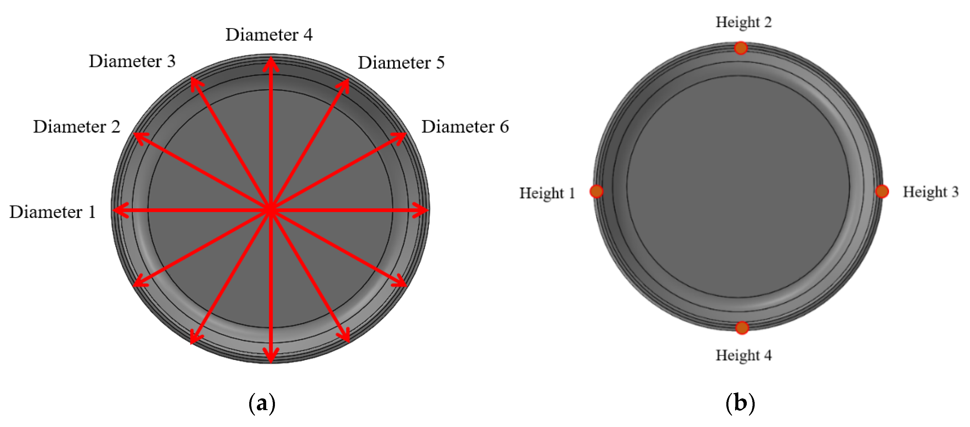
To build an ANN prediction model, the mass, nominal diameter, and height of the injection molded product shown in Figure 1 were measured and considered as output parameters for each injection molding condition shown in Table 4 and Table 5. The mass of the injection molded product was measured by a CUX420H (CAS), a digital weighing scale, and the diameter of the product was determined by the average value of measurements at a total of six points shown in Figure 3a using the Datastar200 (RAM OPTICAL INSTRUMENT), a non-contact optical measuring instrument. The height of the product was determined by the average value of measurements at four points using the Mitutoyo Digimatic Height Gage, as shown in Figure 3b.

3. Building the Model to Predict the Product Qualities

3.1. Artificial Neural Network

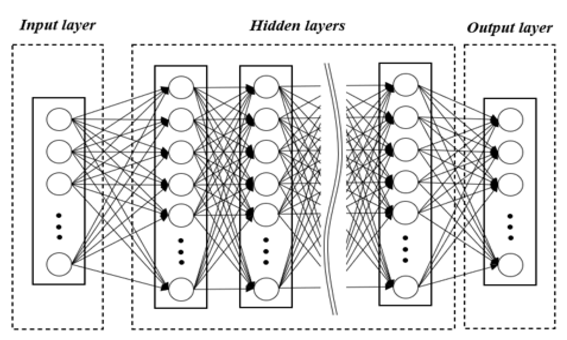
The ANN model mimics the process of the human brain recognizing and solving problems. As in the neural network constituting the human brain, this model has a computational processing structure in which neurons are arranged in each computation layer of the ANN. Figure 4 shows how this ANN structure is connected between input and output parameters. The ANN is an algorithm in which the structure is largely divided into input, hidden, and output layers, and the corresponding neurons are placed on each layer. In addition, a different number of neurons arranged on each layer can be set for each layer [19,20].
The back propagation algorithm is the most common learning method for training ANNs because the calculation and construction of this model are simple. The term “back propagation” refers to errors propagating in the opposite direction of the ANN’s progression. Errors are defined as the difference between output values of ANN and the actual values in the data set. The errors are used to calculate the changes in previous neurons in a backward direction. Thus, the back propagation algorithm requires input and output values of the training data, a method called supervised learning.
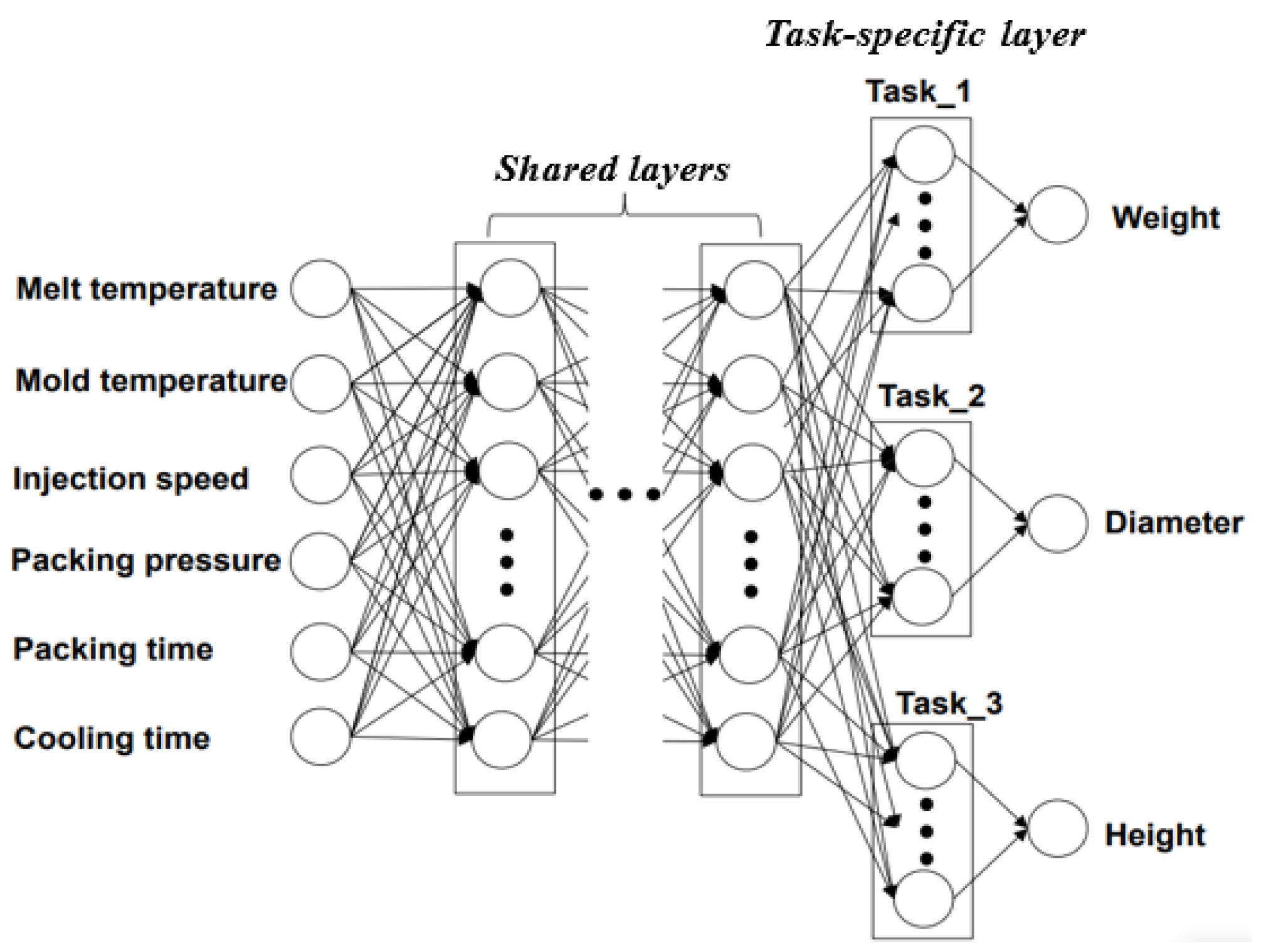
In the present study, an ANN with a MIMO structure was utilized to establish the relationship between multiple input parameters and multiple output parameters, as shown in Figure 5. Furthermore, the multi-task learning technique was applied to the typical MIMO structure shown in Figure 4 by assigning the task-specific layer for each output parameter [21,22]. Moreover, by placing the task-specific layer, which consists of one or more layers, for each output parameter, the root mean square error (RMSE) for each output parameter was individually calculated to minimize the summation of the RMSEs of all output parameters. The conventional MIMO method is known to be difficult to reflect the characteristics of each parameter accurately because the output parameters are related to each other, and all characteristics are learned dependently [22], so this study strived to resolve this issue by using the multi-task learning technique, as described well in other studies [23,24].

3.2. The Search for Optimal Hyper-Parameters

In training a machine learning model using an ANN, parameters that the user must set are called hyper-parameters. Because the initial setting of these parameters determines the efficiency and performance of the ANN, it is important to set the appropriate hyper-parameters according to the purpose of the ANN. Thus, the hyper-band technique [25] was used to determine the range of hyper-parameters, as shown in Table 7. This method is widely used because it requires significantly less time for optimization than conventional techniques, such as the grid search method, random search method, and Bayesian search method. It further showcases the excellent performance of the derived results.

4. Results

4.1. Injection Molding Experiment

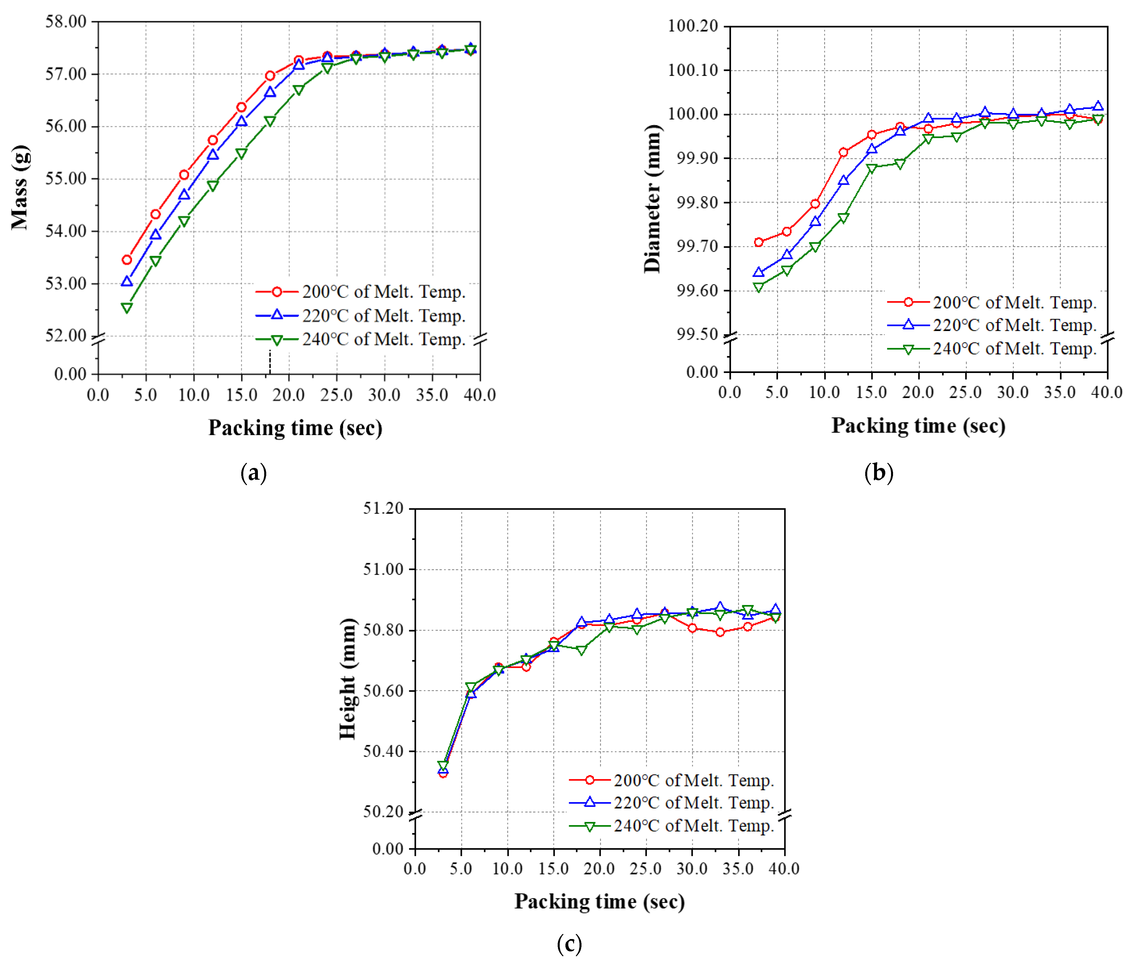
All the measurement results concerning the mass, diameter, and height of the final injection molded product are presented in Table A1 (Appendix A) for the case of the linear relationship between parameters with a packing time ranging from 6.0 s to 18.0 s. Table A2 (Appendix A) shows the injection molding experiments, in which the maximum value of the packing time was extended to 39.0 s among the injection molding conditions. According to the experimental data shown in Figure 6, when applying the packing time of 3.0~39.0 s, clear nonlinearity can be found in all the results of three output parameters, i.e., mass, diameter, and height. In particular, Figure 6a shows clear nonlinearity between the mass of the final injection molded product and packing time, as shown in the preliminary experiment in Figure 2. When the melt temperature was 200 °C, the linear and nonlinear sections were divided by the boundary with a packing time of 18.0 s.
Even though the linear relation was well suited to only one of the output parameters, i.e., the mass of the final product as shown in Figure 2, the packing time of 18.0 s was taken as a useful criterion. For convenience, the ANN model was constructed, and its performance was evaluated by dividing the experiments (or data sets) into two groups depending on the above-mentioned criterion, i.e., the packing time of 18.0 s in the present study. As shown in Table A1 and Table A2, the data groups were divided into a group with a packing time in the range of 3.0~18.0 s (linear relation group) and a group with an extended packing time ranging from 3.0 to 39.0 s (nonlinear relation group).

4.2. The Prediction Models Learned by the Linear Relationship Group (Packing Time ≤ 18.0 s)

In Table A1 and Table A2, a dataset with a packing time between 3.0 and 18.0 s was selected to form a linear relation group as mentioned above, and based on this, an ANN model was constructed. Fifty combinations from Table A1 and 18 combinations from Table A2 were selected to create a “linear relation group” with 68 combinations. Among the selected combination data, 54 combination datasets were used as training data for the ANN model. Seven of the remaining combination data (# 28, 33, 38, 43, 48, 55, 77) were used as validation data sets for the ANN model during training. The other seven combination data were used as test data to evaluate the prediction performance of the final ANN model. When the values of hyper-parameters in Table 8 searched by hyper-band technique were selected, the minimum RMSE value of output parameters could be obtained for the final ANN structure.
The performance of this ANN model was compared to those of a linear regression and a second-order polynomial regression model that used the same training data set calculated by the library (scikit-learn) in the Python package. As a final step, the test data set consisted of experiments #29, 34, 39, 44, 49, 56, and 78 that were applied to the constructed prediction models, and the experimental and prediction results are compared and summarized in Table 9. As seen in Table 9, the RMSE values for mass, diameter, and height of the ANN model were generally lower than those of the linear regression and second-order polynomial regression. We can conclude that the prediction performance of the final ANN model obtained for the linear relation group was relatively better than that of the linear regression and second-order polynomial regression models.
Figure 7 shows the predicted results of three models obtained from the test data and experimental results with error bars calculated by applying ISO20457:2018 (Plastics molded parts—Tolerances and acceptance conditions); the dimensional quality standard for injection-molded products, as well as the mass quality standard for general PP. The calculated standard error equivalent to ISO20457:2018 of the injection molded product used in this study was ±0.009 mm [27] for both diameter and height, and ±0.5% [28] was applied as the standard error of the mass for PP molded product. According to Figure 7, both ANN and linear regression satisfied all the quality standards for the mass, diameter, and height of the present injection molded product. In contrast, in the case of the second-order polynomial regression, several combinations of experimental cases (#39, 44) failed to meet the quality standard for diameter, as shown in Figure 7b.
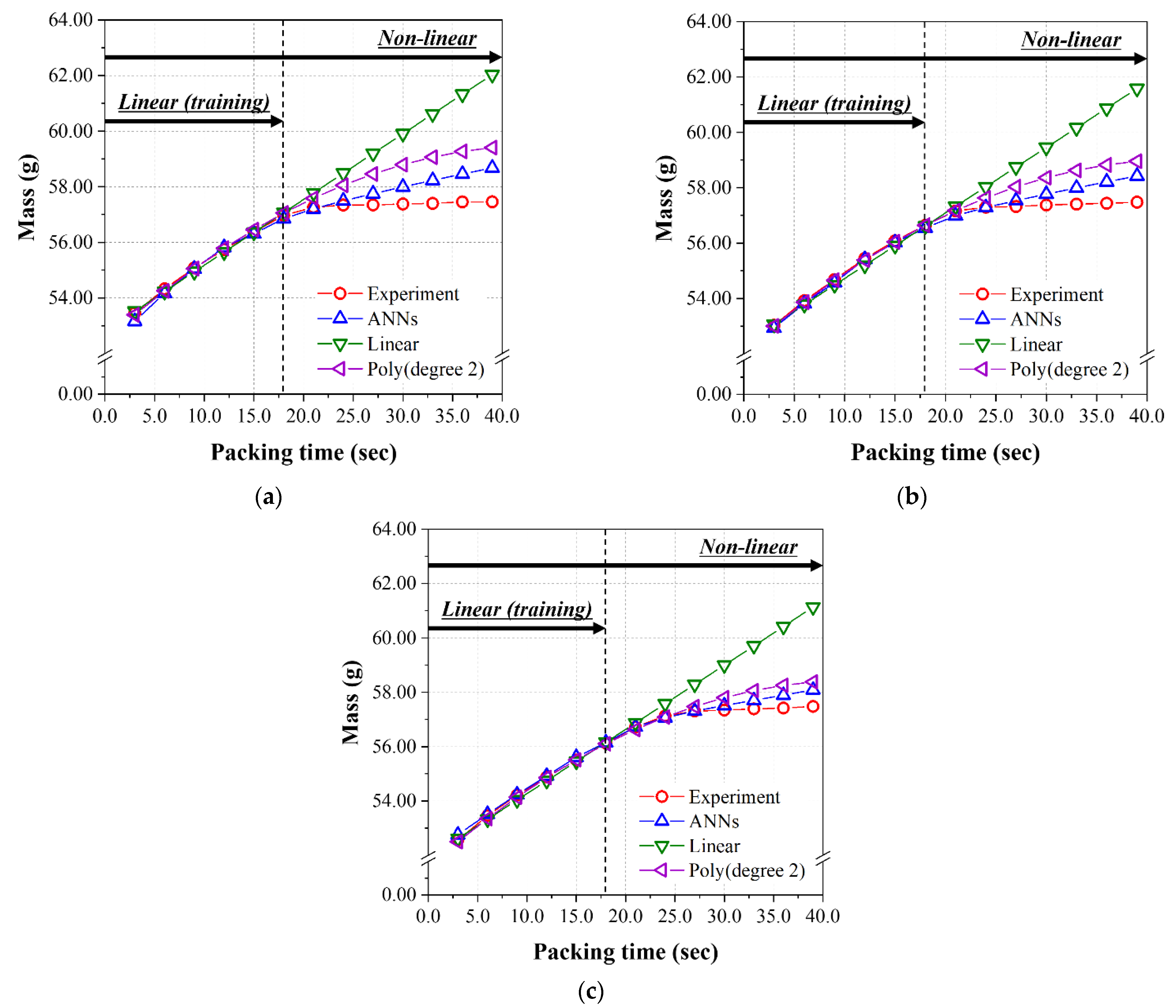
To find the relationship between the input and output parameters in a different way, the predicted results of three models were graphically shown for the data sets in Table A2 as a function of the packing time. Here, the previous test data set (#29, 34, 39, 44, 49, 56, and 78) was substituted for the data set in the linear range for packing time (#51~56, 64~69, 77~82). Figure 8a–c, which were performed at 200 °C, 220 °C, and 240 °C, respectively, show the prediction and experimental results of the final mass as a function of the packing time for the linear range of 3.0~18.0 s and extra range over 18.0 s.
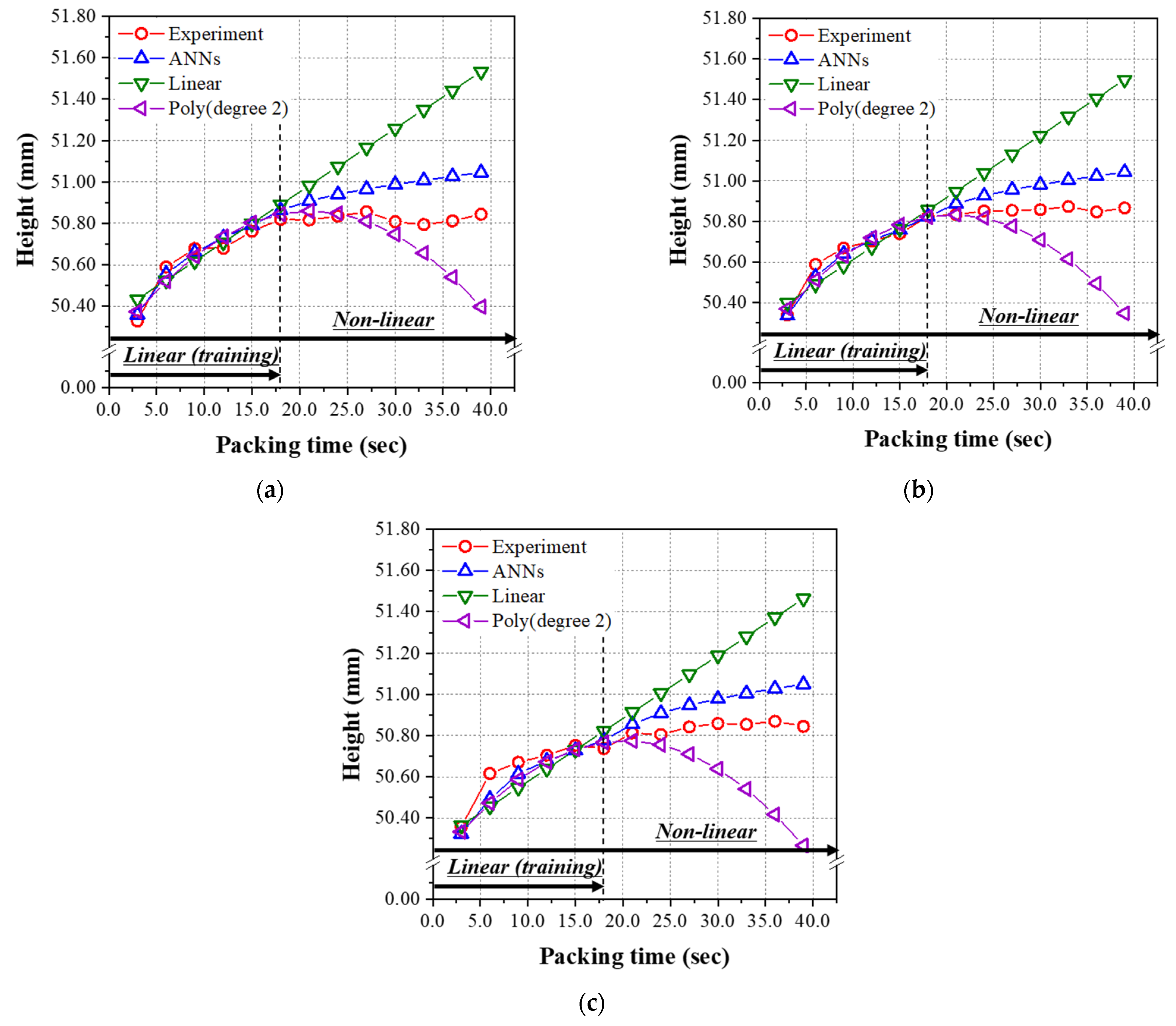
As seen in Table 10, the RMSE values for the mass of all the three models, i.e., the ANN model, the linear regression, and second-order polynomial regression, are very low. Interestingly, the lowest RMSE was found for the case of second-order polynomial regression. The predicted and experimental data for the mass over 18.0 s are illustrated for reference. Similar to the results from the test data set given in Table 9, the ANN model has the minimum and lowest RMSE among those three models for the diameter and height shown in Table 10. Figure 9 and Figure 10 show the prediction and experimental results for diameter and height as a function of the packing time. From the results of the data set in the linear range for packing time (#51~56, 64~69, 77~82), the prediction performance of the final ANN model was excellent by comparing with that of the linear regression and second-order polynomial regression models.

4.3. The Prediction Model Learned by the Non-Linear Relationship Group

A total of 89 combination datasets shown in Table A1 and Table A2 were selected, and 71 combinations were used as training data for the ANN model. 9 of the remaining combinations data (# 28, 33, 38, 43, 48, 58, 70, 73 and 88) were used as validation data for the ANN model during training. The other 9 combination datasets (#29, 34, 39, 44, 49, 59, 71,74, and 89) were used as test data to evaluate the performance of the ANN model. When the hyper-parameter values in Table 11 searched by the hyper-band technique were selected, the minimum RMSE value of output parameters could be obtained for the final ANN structure in the same way as in the linear relation group.
Table 12 compares the RMSE values for the prediction results by applying the test data that were not used to construct the model. The RMSE values of the ANN model for all three output parameters were lower than those of the other models. From the results obtained for this nonlinear relation group, the prediction performance of the final ANN model was much better than that of the linear regression and second-order polynomial regression models.
Figure 11 shows the predicted results of three models obtained from the test data and experimental results with error bars, as shown in Figure 7 for the linear relation group. All the predicted values of the ANN satisfied the standard specifications. In contrast, the predicted values of the linear regression tended to deviate from the quality standard, and there was a significant deviation or error from the experimental value. The predicted values of the second-order polynomial regarding the mass, diameter, and height of the injection molded product tended to be located within the quality standard. In contrast, only two combination datasets (#39, 44 in Figure 11b) deviated from the quality standard.
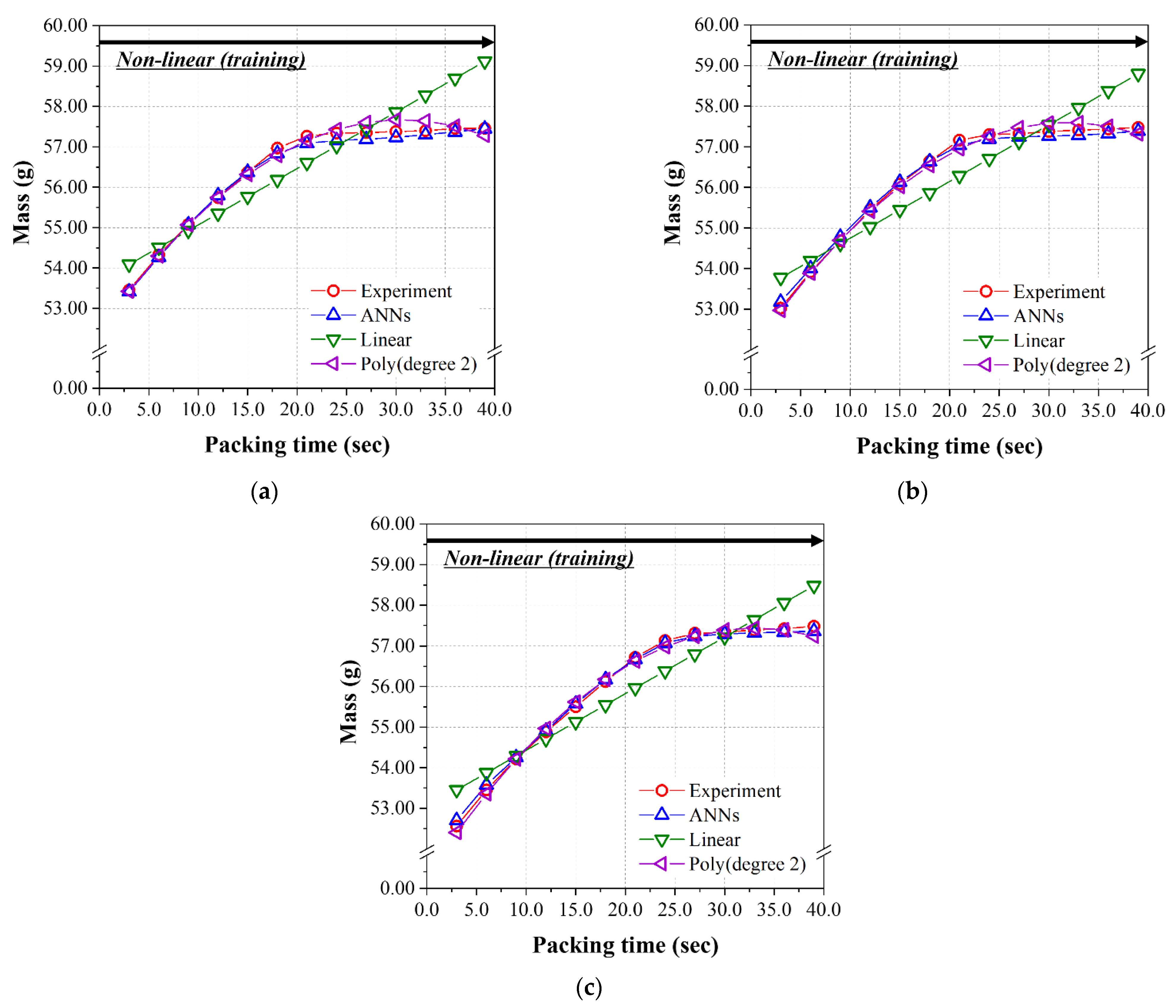
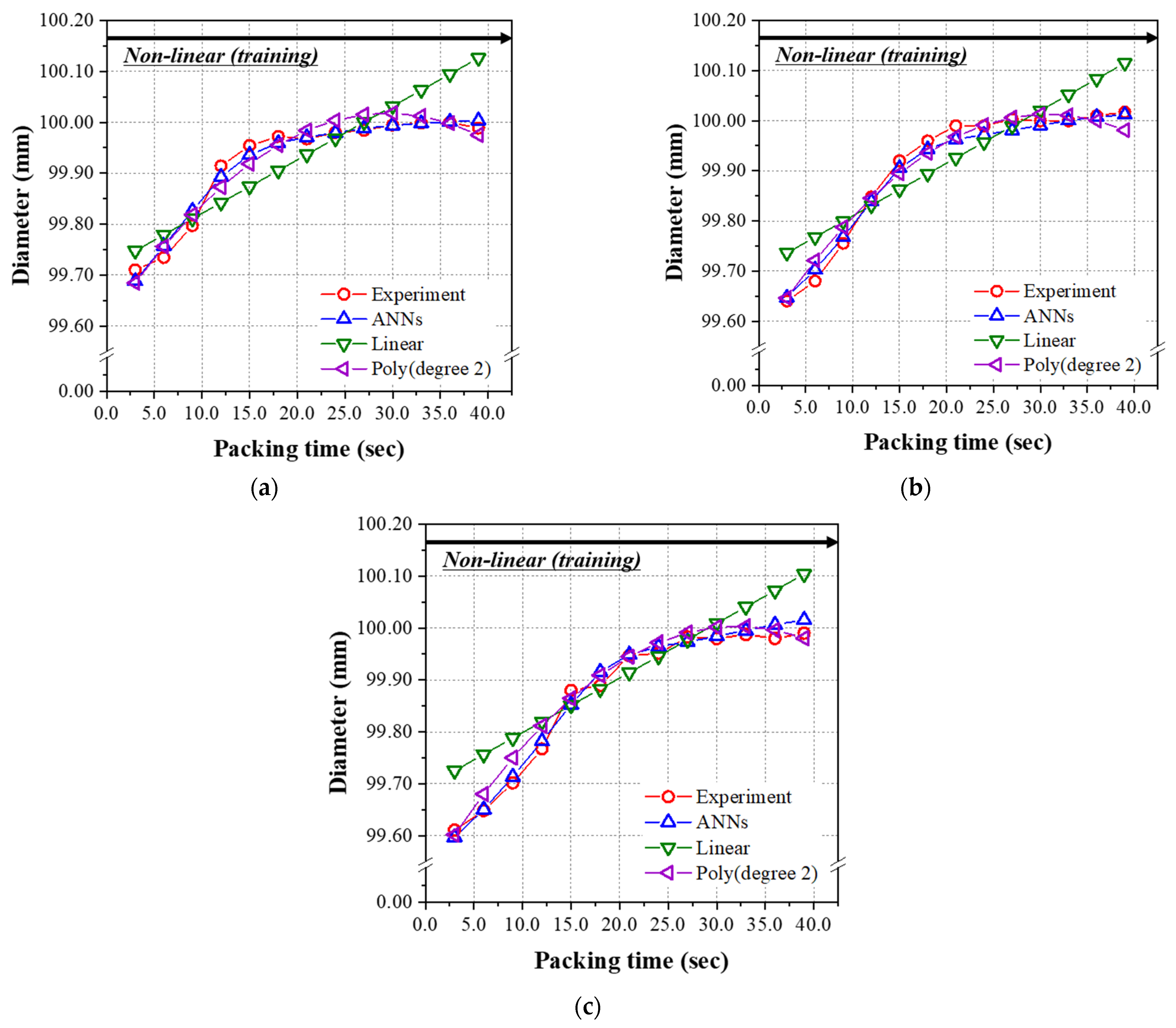
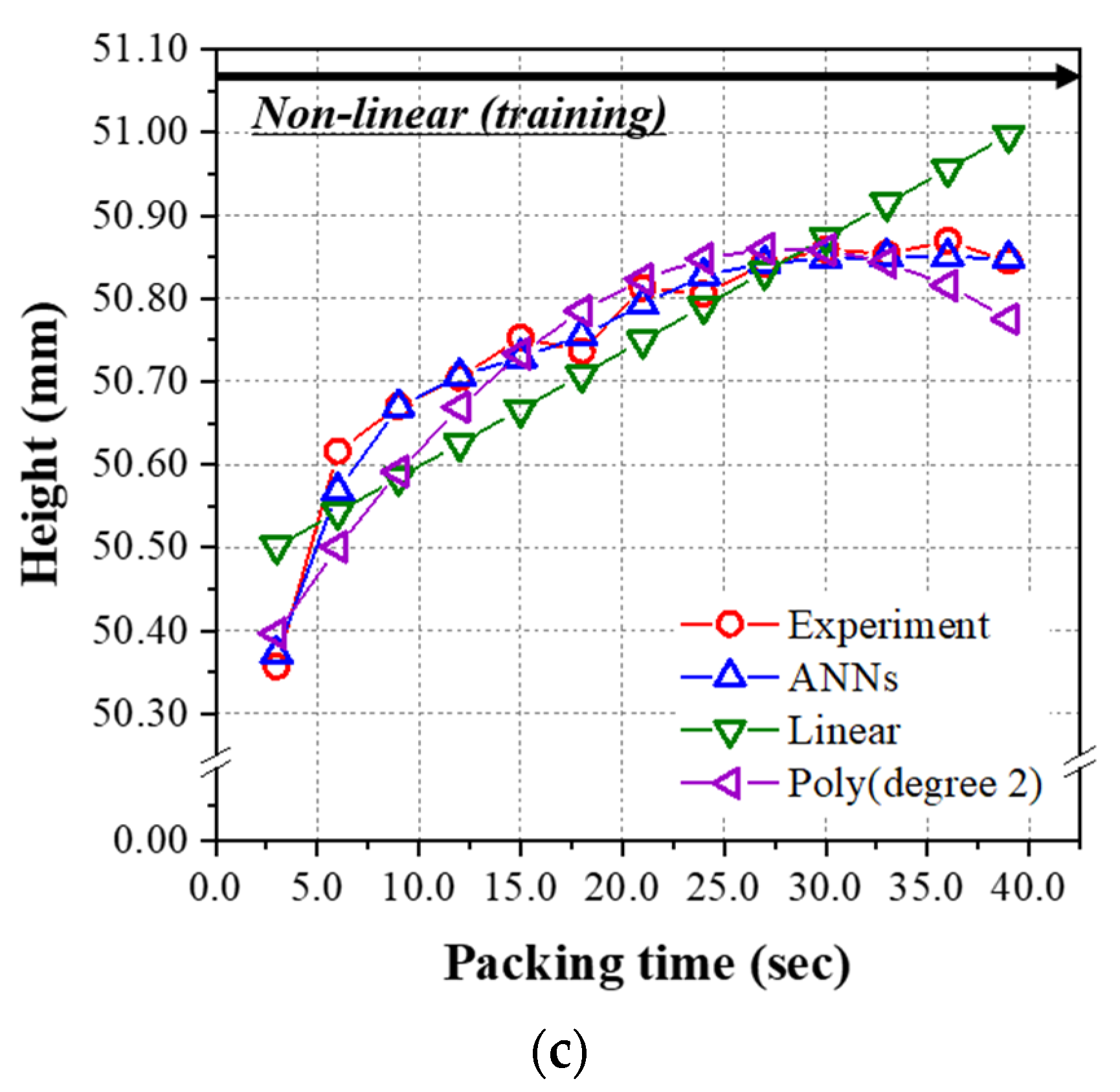
In the analysis of the nonlinear group, the predicted results of three models were graphically shown for the data sets in Table A2 as a function of the packing time up to 39.0 s. The previous test data set (#29, 34, 39, 44, 49, 59, 71,74, and 89) was substituted for the data set, including all the packing times (#51~89). Figure 12a–c, performed at 200 °C, 220 °C, and 240 °C, respectively, show the prediction and experimental results of the final mass as a function of the packing time for the linear range of 3.0~39.0 s. As seen in Table 13, the RMSE values of the mass for the ANN model of 1.709 × 10⁻², and second-order polynomial regression of 2.105 × 10⁻², are low enough to give an excellent prediction. As can be seen in the figures, the performance of the linear regression model is very poor and the RMSE value is very high. Similar to the results obtained from the test data set given in Table 12, the ANN model has the minimum and lowest RMSE among the three models for the diameter and height shown in Table 13. Figure 13 and Figure 14 show the prediction and experimental results for diameter and height as a function of the packing time. From the results of the data set in the nonlinear range for packing time (#51~89) of 3.0 s~39.0 s, the prediction performance of the final ANN model was the best among the three models. While there is a nonlinear relationship between input and output parameters, ANN is the best choice from our limited data sets.

5. Conclusions

Based on the results of the preliminary experiment, the data sets used in the present study were divided into two groups. One showed the linear relation between the mass of the final product and the range of packing time (linear relation group), and the other showed clear nonlinear relation (nonlinear relation group). For convenience, the linear relation group was specified to have the packing time less than or equal to 18.0 s. In other words, the range of the packing time was 3.0 s~18.0 s. The nonlinear relation group includes the data sets having a packing time up to 39.0 s, i.e., the input range of the packing time was 3.0 s~18.0 s.
ANN, linear regression, and second-order polynomial regression models were constructed for the linear and nonlinear groups, respectively. Furthermore, the performance of each predictive model and their ability to represent the relationships between parameters were compared. For the linear relation group, the prediction performance of the ANN model was relatively better than that of the linear regression and second-order polynomial regression models. However, all three models showed low RMSE, while the relation between the mass and the packing time showed high linearity. For the nonlinear relation group, the predicted results of the ANN model constructed in the present study were much better than that of the linear regression and second-order polynomial regression models. The ANN model might be the best method for predicting data concerning the relationship between input and output parameters, i.e., the range of input parameters including the nonlinear zone.
From the analysis of our specific data sets in the present study, ANN might be a better choice than linear or second-order polynomial regression if the data set has the characteristic of both linear and nonlinear. The results of this study might be a useful reference for future studies applying the ANN to the injection molding industry.

Author Contributions

Conceptualization, J.L., K.Y., and J.K; methodology, J.L., K.Y., and J.K; data curation, J.L.; formal analysis, J.L. validation, J.L. and D.Y.; visualization, J.L.; investigation, J.L. and D.Y.; resources, J.L. and D.Y.; writing—original draft preparation, J.L.; writing—review and editing, J.L., K.Y., and J.K. All authors have read and agreed to the published version of the manuscript.

Funding

This research received no external funding.

Institutional Review Board Statement

Not applicable.

Informed Consent Statement

Not applicable.

Data Availability Statement

Not applicable.

Acknowledgments

This work was supported by the Materials/Parts Technology Development Program (Project name: Development of process (injection molding, plating) design advisor for high-quality parts, Project No.: 20013311, KM210513) funded by the Ministry of Trade, Industry, and Energy (MOTIE) of Korea.

Conflicts of Interest

The authors declare no conflict of interest.

Appendix A

Table A1. Product qualities for injection molding conditions with linearity.
No.Mass (g)Diameter (mm)Height (mm)NoteNo.Mass (g)Diameter (mm)Height (mm)Note
154.0599.7750.48L272654.0899.8550.50Random
255.8999.8850.72L272755.2999.9350.68Random
356.9699.8850.82L272856.1699.9150.78Random
454.3399.7350.59L272956.2299.9250.79Random
555.7299.9050.73L273056.0599.9350.78Random
657.1799.9550.88L273154.1199.7950.51Random
754.1399.7450.52L273254.4499.8350.56Random
855.6999.9250.77L273357.07100.0050.92Random
957.15100.0050.92L273453.9699.7350.49Random
1054.2499.6950.57L273557.0699.9350.90Random
1155.9999.9450.82L273654.6899.8450.59Random
1257.31100.0250.95L273755.4999.8650.74Random
1353.2299.7650.43L273854.0799.7950.51Random
1454.8699.9050.61L273956.0299.9950.75Random
1555.9799.9150.74L274056.0499.9650.78Random
1653.7599.7750.45L274154.9299.8950.65Random
1755.2599.8850.67L274256.93100.0150.92Random
1856.2299.8950.77L274356.53100.0250.85Random
1953.3899.6450.45L274455.5899.9650.75Random
2054.8799.9250.67L274556.12100.0250.81Random
2156.30100.0250.86L274654.3199.8150.56Random
2253.8999.7150.51L274753.5299.7950.43Random
2355.2299.9450.73L274854.7399.9450.61Random
2456.60100.0550.92L274954.4799.8050.61Random
2552.6499.6650.26L275053.8099.7850.52Random
Table A2. Product qualities for injection molding conditions with nonlinearity according to packing time.
No.Mass (g)Diameter (mm)Height (mm)No.Mass (g)Diameter (mm)Height (mm)
5153.4699.7150.337157.3099.9950.85
5254.3399.7350.597257.32100.0050.85
5355.0899.8050.687357.38100.0050.86
5455.7499.9150.687457.41100.0050.87
5556.3799.9550.767557.44100.0150.85
5656.9799.9750.827657.48100.0250.87
5757.2799.9750.827752.5699.6150.36
5857.3499.9850.837853.4699.6550.52
5957.3599.9850.867954.2299.7050.67
6057.3899.9950.818054.8999.7750.70
6157.40100.0050.798155.5199.8850.75
6257.46100.0050.818256.1399.8950.74
6357.4699.9950.848356.7299.9550.81
6453.0399.6450.348457.1499.9550.81
6553.9299.6850.598557.3199.9850.84
6654.6899.7650.678657.3599.9850.86
6755.4599.8550.708757.3999.9950.85
6856.0899.9250.748857.4299.9850.87
6956.6499.9650.838957.4899.9950.85
7057.1699.9950.83

References

  1. Rosato, D.V.; Rosato, M.G. Injection Molding Handbook; Springer Science & Business Media: Berlin, Germany, 2012. [Google Scholar]
  2. Fernandes, C.; Pontes, A.J.; Viana, J.C.; Gaspar-Cunha, A. Modeling and optimization of the injection-molding process: A review. Adv. Polym. Technol. 2018, 37, 429–449. [Google Scholar] [CrossRef]
  3. Shen, C.; Wang, L.; Li, Q. Optimization of injection molding process parameters using combination of artificial neural network and genetic algorithm method. J. Mater. Process. Technol. 2007, 183, 412–418. [Google Scholar] [CrossRef]
  4. Zink, B.; Szabó, F.; Hatos, I.; Suplicz, A.; Kovács, N.K.; Hargitai, H.; Tábi, T.; Kovács, J.G. Enhanced injection molding simulation of advanced injection molds. Polymers 2017, 9, 77. [Google Scholar] [CrossRef] [PubMed] [Green Version]
  5. Hentati, F.; Hadriche, I.; Masmoudi, N.; Bradai, C. Optimization of the injection molding process for the PC/ABS parts by integrating Taguchi approach and CAE simulation. Int. J. Adv. Manuf. Technol. 2019, 104, 4353–4363. [Google Scholar] [CrossRef]
  6. Lee, J.H.; Bae, H.S.; Kwak, J.S. Dimensional optimization of electric component in ultra thin-wall injection molding by using Moldflow simulation. J. Korean Soc. Manuf. Process Eng. 2020, 19, 1–6. [Google Scholar] [CrossRef]
  7. Ozcelik, B.; Erzurumlu, T. Comparison of the warpage optimization in the plastic injection molding using ANOVA, neural network model and genetic algorithm. J. Mater. Process. Technol. 2006, 171, 437–445. [Google Scholar] [CrossRef]
  8. Yin, F.; Mao, H.; Hua, L.; Guo, W.; Shu, M. Back propagation neural network modeling for warpage prediction and optimization of plastic products during injection molding. Mater. Des. 2011, 32, 1844–1850. [Google Scholar] [CrossRef]
  9. Yang, D.C.; Lee, J.H.; Yoon, K.H.; Kim, J.S. A study on the prediction of optimized injection molding condition using artificial neural network(ANN). Trans. Mater. Process. 2020, 4, 218–228. [Google Scholar] [CrossRef]
  10. Lee, C.H.; Na, J.W.; Park, K.H.; Yu, H.J.; Kim, J.S.; Choi, K.W.; Park, D.Y.; Park, S.J.; Rho, J.S.; Lee, S.C. Development of artificial neural network system to recommend process conditions of injection molding for various geometries. Adv. Intell. Sys. 2020, 2, 1–14. [Google Scholar] [CrossRef]
  11. Gim, J.; Rhee, B. Novel Analysis Methodology of Cavity Pressure Profiles in Injection-Molding Processes Using Interpretation of Mchine Learning Model. Polymers 2021, 13, 3297. [Google Scholar] [CrossRef]
  12. Abdul, R.; Guo, G.; Chen, J.C.; Yoo, J.J.W. Shrinkage prediction of injection molded high polyethylene parts with taguchi/artificial neural network hybrid experimental design. Int. J. Interact. Des. Manuf. 2020, 14, 345–357. [Google Scholar] [CrossRef]
  13. Heinisch, J.; Lockner, Y.; Hopmann, C. Comparison of design of experiment methods for modeling injection molding experiments using artificial neural networks. J. Manuf. Process. 2021, 61, 357–368. [Google Scholar] [CrossRef]
  14. Ke, K.C.; Huang, M.S. Quality Prediction for Injection Molding by Using a Multilayer Perceptron Neural Network. Polymers 2020, 12, 1812. [Google Scholar] [CrossRef]
  15. Huang, Y.M.; Jong, W.R.; Chen, S.C. Transfer Learning Applied to Characteristic Prediction of Injection Molded Products. Polymers 2021, 13, 3874. [Google Scholar] [CrossRef] [PubMed]
  16. Moayyedian, M.; Dinc, A.; Mamedov, A. Optimization of Injection-Molding Process for Thin-Walled Polypropylene Part Using Artificial Neural Network and Taguchi Techniques. Polymers 2021, 13, 4158. [Google Scholar] [CrossRef] [PubMed]
  17. Yang, D.C.; Lee, J.H.; Yoon, K.H.; Kim, J.S. A study on the practical application of the integrated ANN system for manufacturing the target quality of the injection molded product. Korea-Aust. Rheol. J. 2022, 1–11. [Google Scholar] [CrossRef]
  18. De Villiers, J.; Barnard, E. Backpropagation neural nets with one and two hidden layers. IEEE Trans. Neural Netw. 1993, 4, 136–141. [Google Scholar] [CrossRef]
  19. Goodfellow, I.; Bengio, Y.; Courville, A. Deep Learning (Adaptive Computation and Machine Learning Series); MIT Press: Cambridge, MA, USA, 2017. [Google Scholar]
  20. Reed, R.; Marksll, R.J. Neural Smithing: Supervised Learning in Feedforward Artificial Neural Networks; MIT Press: Cambridge, MA, USA, 1999. [Google Scholar]
  21. Rudder, S. An overview of multi-task learning in deep neural networks. arXiv 2017, arXiv:1706.05098. [Google Scholar] [CrossRef]
  22. Zhang, Y.; Yang, Q. An overview of multi-task learning. Natl. Sci. Rev. 2018, 5, 30–43. [Google Scholar] [CrossRef] [Green Version]
  23. Wan, Z.; Yu, Z.; Shu, L.; Zhao, Y.; Zhang, H.; Xu, K. Intelligent optical performance monitor using multi-task learning based artificial neural network. Opt. Express 2019, 27, 11281–11291. [Google Scholar] [CrossRef] [Green Version]
  24. Michelucci, U.; Venturini, F. Multi-task learning for multi-dimensional regression: Application to luminescence sensing. Appl. Sci. 2019, 9, 4748. [Google Scholar] [CrossRef] [Green Version]
  25. Li, L.; Jamieson, K.; DeSalvo, G.; Rostamizadeh, A.; Talwalkar, A. Hyperband: A novel bandit-based approach to hyper-parameter optimization. J. Mach. Learn. Res. 2017, 18, 6765–6816. [Google Scholar]
  26. Kingma, D.P.; Ba, J. Adam: A method for stochastic optimization. arXiv 2014, arXiv:1412.6980. [Google Scholar] [CrossRef]
  27. ISO 20457:2018; Plastics Moulded Parts—Tolerances and Acceptance Conditions. ISO: Geneva, Switzerland, 2018.
  28. Yang, D.C. A Study on the Injection Molding Conditions for Manufacturing Target Quality Product Using Artificial Neural Network. Master’s Thesis, Dankook University, Yongin, Korea, 2021. Available online: http://lib.dankook.ac.kr/dcollection/common/orgView/000000196386 (accessed on 14 March 2022).
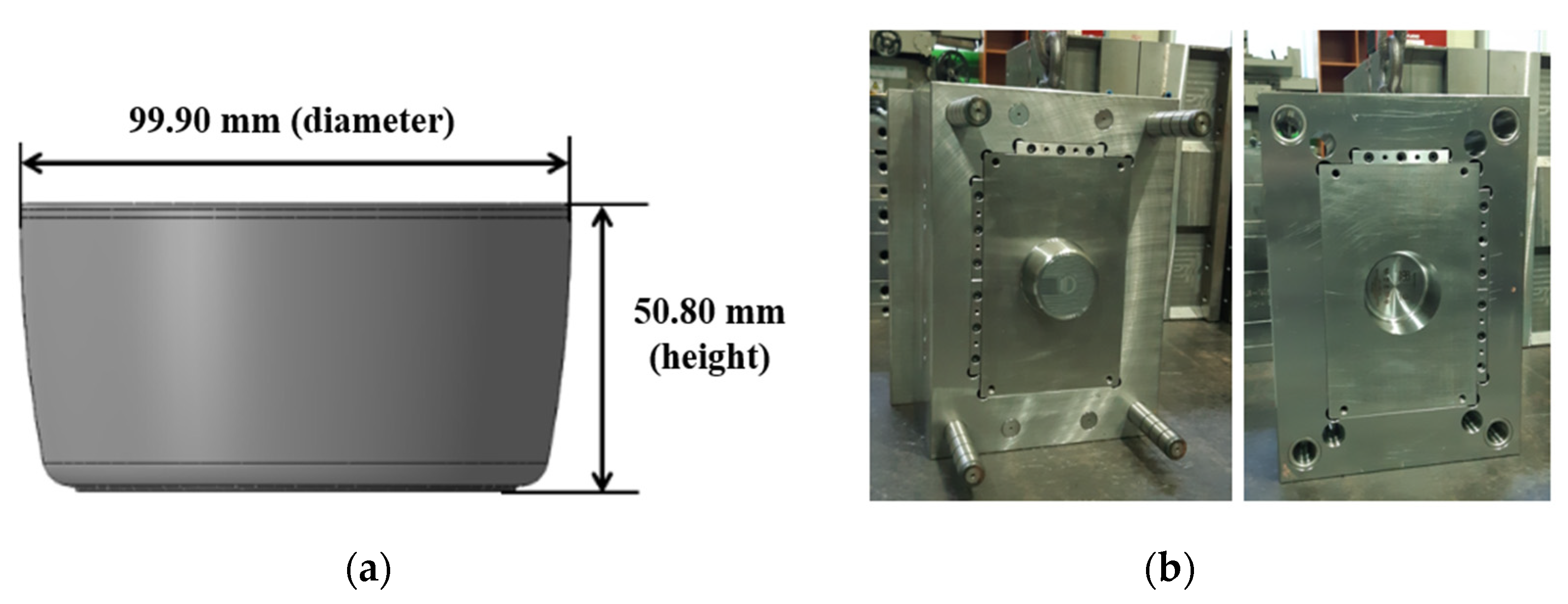
Figure 1. Images of (a) the rice bowl and (b) the mold.
Polymers 14 01724 g001
Figure 2. Results of the preliminary experiment to show linear and nonlinear relation between packing time and mass.
Polymers 14 01724 g002
Figure 3. Measurement points for (a) diameter and (b) height.
Polymers 14 01724 g003
Figure 4. Schematic of the structure of the artificial neural network (ANN).
Polymers 14 01724 g004
Figure 5. The multi-input multi-output (MIMO) structure using multi-task learning in the present study (hard parameter sharing) [21,22].
Polymers 14 01724 g005
Figure 6. Experimental measurement results for the process conditions of Table 5 showing nonlinearity (packing time: 3.0~39.0 s): (a) mass, (b) diameter, and (c) height.
Polymers 14 01724 g006
Figure 7. Performances of the prediction models using test data learned by the linear relation group (packing time was 3.0~18.0 s): (a) mass, (b) diameter, and (c) height.
Polymers 14 01724 g007
Figure 8. Predicted mass of nonlinear relation group from Table A2 using the models learned by the linear relation group (packing time was 3.0–18.0 s). Melt temperatures; (a) 200 °C, (b) 220 °C, and (c) 240 °C.
Polymers 14 01724 g008
Figure 9. Predicted diameters of the nonlinear relation group from Table A2 using the models learned by the linear relation group (packing time was 3.0~18.0 s). Melt temperatures; (a) 200 °C, (b) 220 °C, and (c) 240 °C.
Polymers 14 01724 g009
Figure 10. Predicted heights of the nonlinear relation group from Table A2 using the models learned by the linear relation group (packing time was 3.0~18.0 s). Melt temperatures; (a) 200 °C, (b) 220 °C, and (c) 240 °C.
Polymers 14 01724 g010
Figure 11. Performances of the prediction models using test data learned by the nonlinear relation group (packing time was 3.0–39.0 s): (a) mass, (b) diameter, and (c) height.
Polymers 14 01724 g011
Figure 12. Predicted mass of the nonlinear group from Table A2 using the models learned by the nonlinear group (packing time was 3.0–39.0 s). Melt temperatures were (a) 200 °C, (b) 220 °C, and (c) 240 °C.
Polymers 14 01724 g012
Figure 13. Predicted diameters of the nonlinear group from Table A2 using the models learned by the nonlinear group (packing time was 3.0–39.0 s). Melt temperatures were (a) 200 °C, (b) 220 °C, and (c) 240 °C.
Polymers 14 01724 g013
Figure 14. Predicted heights of the nonlinear group from Table A2 using the models learned by the nonlinear group (packing time was 3.0–39.0 s). Melt temperatures were (a) 200 °C, (b) 220 °C, and (c) 240 °C.
Polymers 14 01724 g014aPolymers 14 01724 g014b
Table 1. Previous research on ANNs applied to the injection molding process [7,8,9,10,11,12,13,14,15,16,17].
AuthorProductInput
Parameters
Output
Parameters
The Number of Hidden LayersThe Number of Neurons per Hidden Layers
Ozcelik, B et al.
[7]
Thin shell part
(CAE)
5
(Mold Temp., Melt Temp., Packing pressure, Packing time, Cooling time)
1
(Warpage)
2 hidden layers9 (1st)–9 (2nd)
Yin, F et al.
[8]
Automobile glove component
(CAE)
5
(Mold Temp., Melt Temp., Packing pressure, Packing time, Cooling time)
1
(Warpage)
2 hidden layers20 (1st)–20 (2nd)
Yang, D. C. et al.
[9]
Cup
(experiment)
10
(Melt Temp., Mold Temp., Injection speed, V/P switchover pressure, Packing pressure, Packing time, Cooling time, Back pressure, Plastification speed, Suck back)
1
(Mass)
2 hidden layers43 (1st)–40 (2nd)
Lee, C.H et al.
[10]
36 different products
(CAE, experiment)
9
(Overall volume, Cavity volume, Overall surface area, Cavity surface area, Filling time, Melt Temp., Mold Temp., Packing pressure, Packing time)
1
(Weight)
2 hidden layers28 (1st)–28 (2nd)
Gim, J. et al.
[11]
Spiral
(experiment)
10
(Time and pressure value from sensor)
1
(Part weight)
1 hidden layer8
Abdul, R et al.
[12]
Tensile specimens
(experiment)
3
(Injection speed, Holding time, Cooling time)
2
(Length shrinkage, Width shrinkage)
1 hidden layer4 (1st)
Heinisch, J et al.
[13]
Plate
(CAE)
6
(Mold Temp., Melt Temp., Injection time, Packing pressure, Packing time, Cooling time)
3
(Weight, length, width)
1 hidden layer5 (1st)
Ke, K. C. et al.
[14]
IC tray
(experiment)
1~11
(Combinations of 11 pressure sensor signal)
3 points of width1 hidden layer1~33 (1st)
Huang, Y. M. et al.
[15]
Circle plate
(CAE)
5
(Injection speed, Packing time, Mold Temp., Melt Temp.)
3
(Injection pressure, Cooling time, Z shrinkage)
2 hidden layers7 (1st)–3 (2nd)
5
(Injection pressure, Cooling time, X, Y, Z shrinkage)
2 hidden layers11 (1st)–7 (2nd)
Moayyedian, M. et al.
[16]
Circle plate
(CAE)
4
(Filing time, Cooling time, Packing time, Melt temperature)
3
(Short shot, Shrinkage rate, Warpage)
Not mentionedNot mentioned
Yang, D. C. et al.
[17]
LEGO
(experiment)
8
(Melt Temp., Mold Temp., Injection speed, Packing pressure, Packing time, Cooling time, Back pressure, Screw speed)
5
(Mass, Pressure at the end of fill, X, Y, Z Length)
1 hidden layer11 (1st)
Table 2. General properties of the polypropylene (PP) used in this study (LUPOL GP1007F, LG Chemical Co., Ltd.).
PropertiesStandardConditionUnitValue
PhysicalSpecific gravityASTM D792--0.94
Melt flow rateASTM D1238230 °C,
2.16 kg
g/10 min13.0
MechanicalTensile strength
(3.2 mm)
ASTM D63850 mm/minkgf/cm2270
Flexural strength
(6.4 mm)
ASTM D79010 mm/minkgf/cm2360
ThermalHeat deflection Temp. (6.4 mm)ASTM D6484.6 kg°C125
Table 3. Specifications of the injection molding machine (LGEII-150, LSMtron).
ItemValueUnit
Clamping force150ton
Screw diameter32.0mm
Max. injection speed1000mm/s
Max. injection pressure3500bar
Max. injection stroke120mm
Table 4. Process conditions and levels for the experiment.
ConditionsLevel 1Level 2Level 3
Melt temperature (°C)200220240
Mold temperature (°C)405060
Injection speed (mm/s)4070100
Packing pressure (bar)150200250
Packing time (s)6.012.018.0
Cooling time (s)384858
Table 5. Injection molding conditions of linear relation group.
Exp.
No.
Melt
Temperature (°C)
Mold
Temperature (°C)
Injection Speed
(mm/s)
Packing
Pressure (bar)
Packing Time
(s)
Cooling Time
(s)
Note
12004040.01506.038L27
22004040.015012.048L27
32004040.015018.058L27
42005070.02006.038L27
52005070.020012.048L27
62005070.020018.058L27
720060100.02506.038L27
820060100.025012.048L27
920060100.025018.058L27
102204070.02506.048L27
112204070.025012.058L27
122204070.025018.038L27
1322050100.01506.048L27
1422050100.015012.058L27
1522050100.015018.038L27
162206040.02006.048L27
172206040.020012.058L27
182206040.020018.038L27
1924040100.02006.058L27
2024040100.020012.038L27
2124040100.020018.048L27
222404040.02506.058L27
232405040.025012.038L27
242405040.025018.048L27
252406070.01506.058L27
262406070.015012.038L27
272406070.015018.048L27
282145582.720416.352Random
292044443.420213.941Random
302034693.620513.745Random
312025483.42136.648Random
322064361.62216.939Random
332124453.324017.052Random
342125190.82246.148Random
352005250.021517.639Random
362295146.215311.745Random
372284953.221712.358Random
382225163.71678.751Random
392195041.415616.352Random
402284696.515416.757Random
412284662.519110.946Random
422194298.423717.941Random
432204355.824114.844Random
442334250.819813.555Random
452385341.622117.240Random
462344868.22228.841Random
472334484.91716.755Random
482344356.917611.148Random
492394941.22348.652Random
502404976.12416.451Random
Table 6. Injection molding conditions of nonlinear relation group.
Exp.
No.
Melt
Temperature (°C)
Mold
Temperature (°C)
Injection Speed
(mm/s)
Packing
Pressure (bar)
Packing Time
(s)
Cooling Time
(s)
Note
51–
63
20050702003.0–39.0
(interval: 3)
38Non-linear case
64–
76
22050702003.0–39.0
(interval: 3)
38Non-linear case
77–
89
24050702003.0–39.0
(interval: 3)
38Non-linear case
Table 7. Ranges of hyper-parameters obtained by hyper-band technique [25].
Hyper-ParametersRangeNote
Seed number0–50 Step size was 1
Batch size16, 32, 64, …Increased in multiples of 2 until it could cover the number of learning data
OptimizerAdams [26]Fixed
Learning rate0.0001–0.01 [26]Step size was 0.0001
Beta 10.1–1.0 [26]Step size was 0.1
Bata 20.9, 0.99, 0.999, 0.999 [26]-
Number of hidden layers1–5 (shared layers)
1 (task-specific layer)
Step size was 1
(task-specific layer was fixed as one layer)
Number of neurons3–18Step size was 1
InitializerHe normal (hidden layer)
Xavier normal (output layer)
-
Activation functionElu (hidden layer)
Linear (output layer)
-
Drop number0.0–0.4Step size was 0.1
Coefficient of batch normalization0.001, 0.01, 0.1-
Table 8. Optimized hyper-parameters for the linear relationship group.
Hyper-ParametersValue
Seed number16
Batch size16
OptimizerAdams
Learning rate0.0069
Beta 10.6
Beta 20.9
Number of hidden layers3 (shared layers)
1 (specific-task layer)
Number of neurons17–13–13 (shared layers)
13 (specific-task layers for mass)
9 (specific-task layers for diameter)
8 (specific-task layers for height)
InitializerHe normal (hidden layers)
Xavier normal (output layer)
Activation functionElu
Drop number0.0–0.2–0.2 (shared layers)
0.0 (specific-task layers for mass)
0.3 (specific-task layers for diameter)
0.3 (specific-task layers for height)
Coefficient of batch normalization0.001 (mass), 0.01 (diameter), 0.001 (height)
Table 9. Root mean square errors (RMSEs) of normalized test data for prediction models learned by the linear relation group (packing time was 3.0–18.0 s).
Prediction ModelRMSE
MassDiameterHeight
ANN 1.279 × 10 2 6.283 × 10 2 2.467 × 10 2
Linear regression 1.440 × 10 2 8.834 × 10 2 4.860 × 10 2
Polynomial regression of degree 2 1.317 × 10 2 1.360 × 10 1 3.362 × 10 2
Table 10. Root mean square errors (RMSEs) of normalized Table A2 (packing time was 3.0~18.0 s) for prediction models learned by the linear relation group (packing time was 3.0~18.0 s).
Prediction ModelRMSE
MassDiameterHeight
ANN 1.871 × 10 2 3.090 × 10 2 3.925 × 10 2
Linear regression 8.240 × 10 2 7.821 × 10 2
Polynomial regression of degree 2 9.294 × 10 3 7.101 × 10 2 5.218 × 10 2
Table 11. Optimized hyper-parameters for the nonlinear relationship group (packing time was 3.0~39.0 s).
Hyper-ParametersValue
Seed number35
Batch size16
OptimizerAdams
Learning rate0.0073
Beta 10.5
Beta 20.9
Number of hidden layers2 (shared layers)
1 (specific-task layer)
Number of neurons6–5 (shared layers)
4 (specific-task layers for mass)
3 (specific-task layers for diameter)
4 (specific-task layers for height)
InitializerHe normal (hidden layers)
Xavier normal (output layer)
Activation functionElu
Drop number0.0–0.0 (shared layers)
0.2 (specific-task layers for mass)
0.1 (specific-task layers for diameter)
0.0 (specific-task layers for height)
Coefficient of batch normalization0.001 (mass), 0.01 (diameter), 0.001 (height)
Table 12. Root mean square errors (RMSEs) of normalized test data for prediction models learned by the nonlinear relation group (packing time was 3.0–39.0 s).
Prediction ModelRMSE
MassDiameterHeight
ANN 1.966 × 10 2 5.453 × 10 2 2.917 × 10 2
Linear regression 8.427 × 10 2 1.283 × 10 1 9.514 × 10 2
Polynomial regression of degree 2 2.702 × 10 2 9.848 × 10 2 4.436 × 10 2
Table 13. Root mean square errors (RMSEs) of normalized Table A2 (packing time was 3.0~39.0 s) for prediction models learned by the nonlinear group (packing time was 3.0~39.0 s).
Prediction ModelRMSE
MassDiameterHeight
ANN 1.709 × 10 2 2.871 × 10 2 2.578 × 10 2
Linear regression 1.096 × 10 1 1.193 × 10 1 1.084 × 10 1
Polynomial regression of degree 2 2.105 × 10 2 4.273 × 10 2 5.081 × 10 2
Publisher’s Note: MDPI stays neutral with regard to jurisdictional claims in published maps and institutional affiliations.