
Preparation and Performance Improvement Mechanism Investigation of High-Performance Cementitious Grout Material for Semi-Flexible Pavement


Abstract
:1. Introduction
2. Materials and Methods
2.1. Materials
2.1.1. Asphalt
2.1.2. Cement
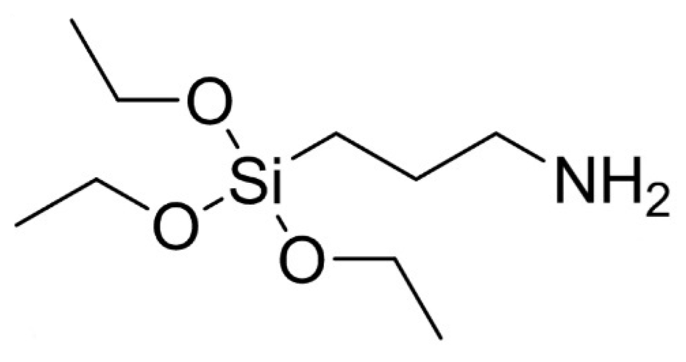
2.1.3. Modifiers
2.2. Methods
2.2.1. Design of the Base Asphalt Mixture Ratio
2.2.2. Design of the Cement-Based Grouting Material Ratio and Determination of the Grouting Volume
2.2.3. Preparation Process
- Preparation of cement-based grouting material
- 2.
- Preparation of base asphalt mixture
- 3.
- SFPM preparation
2.3. Tests
2.3.1. Performance Test
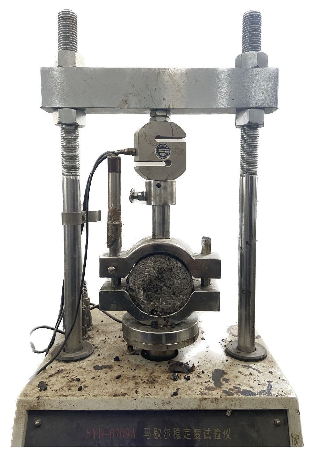
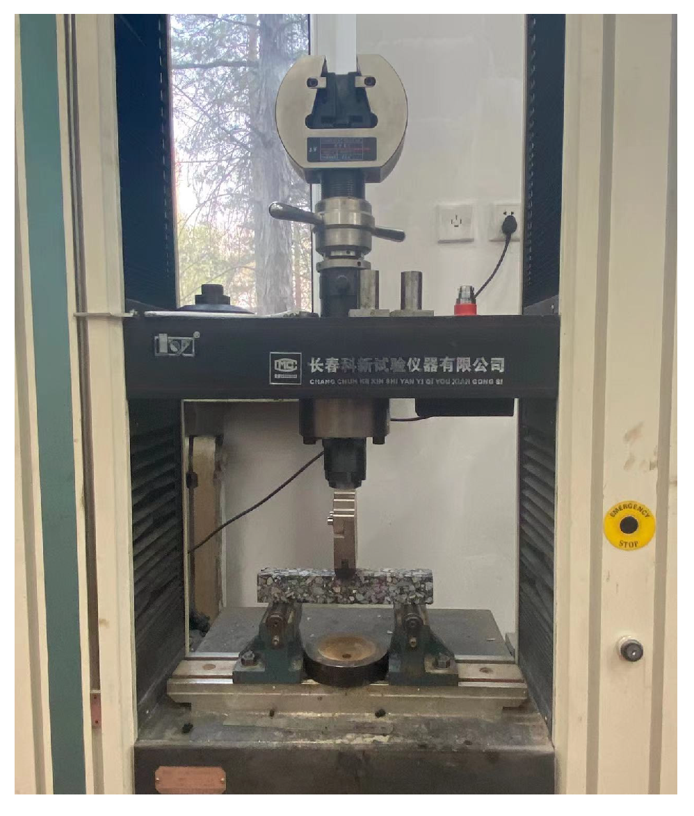
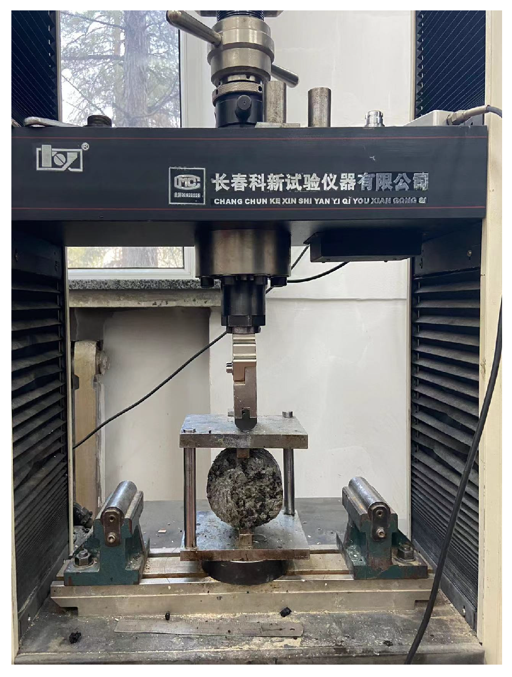
2.3.2. Mechanical Test
- (1)
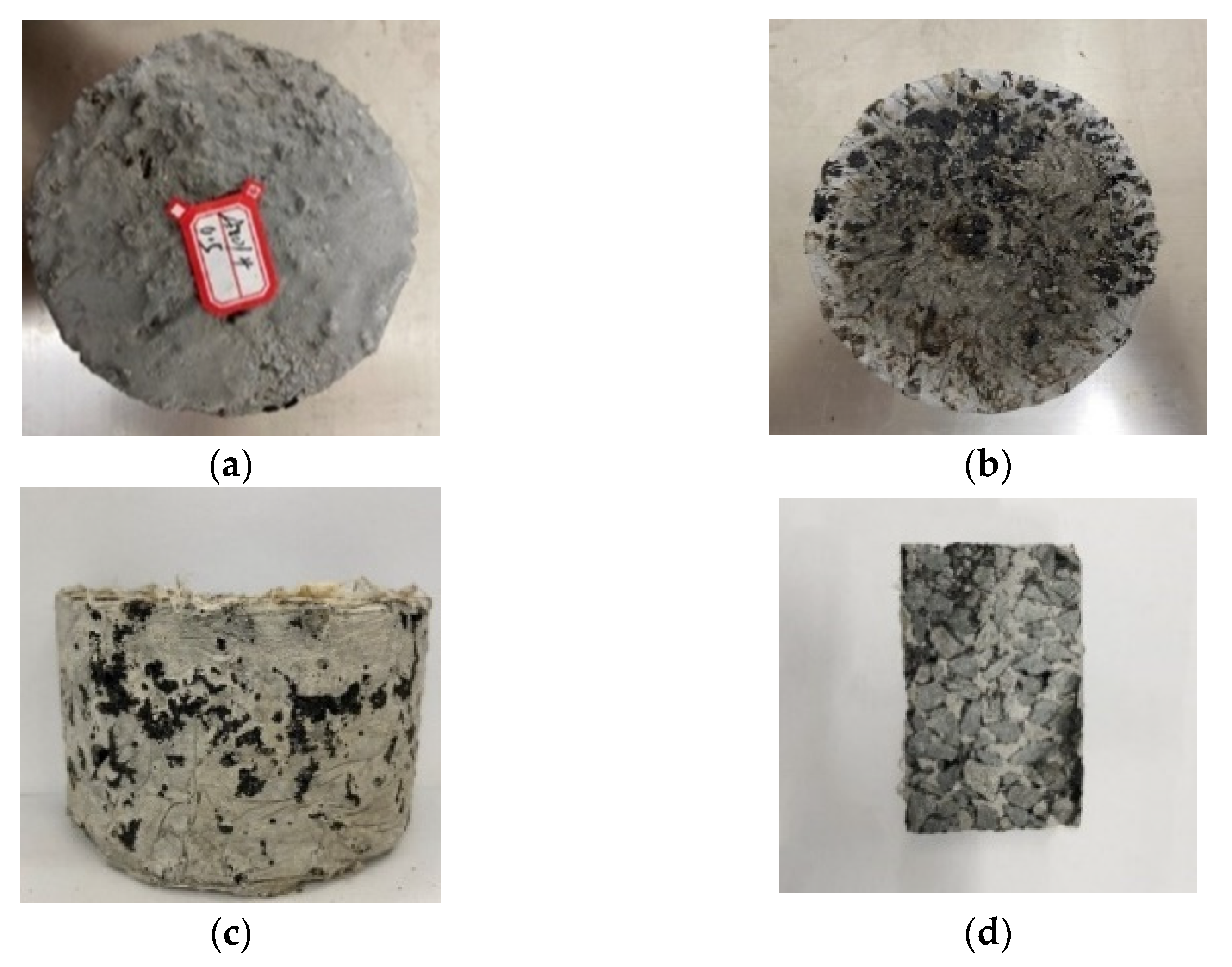
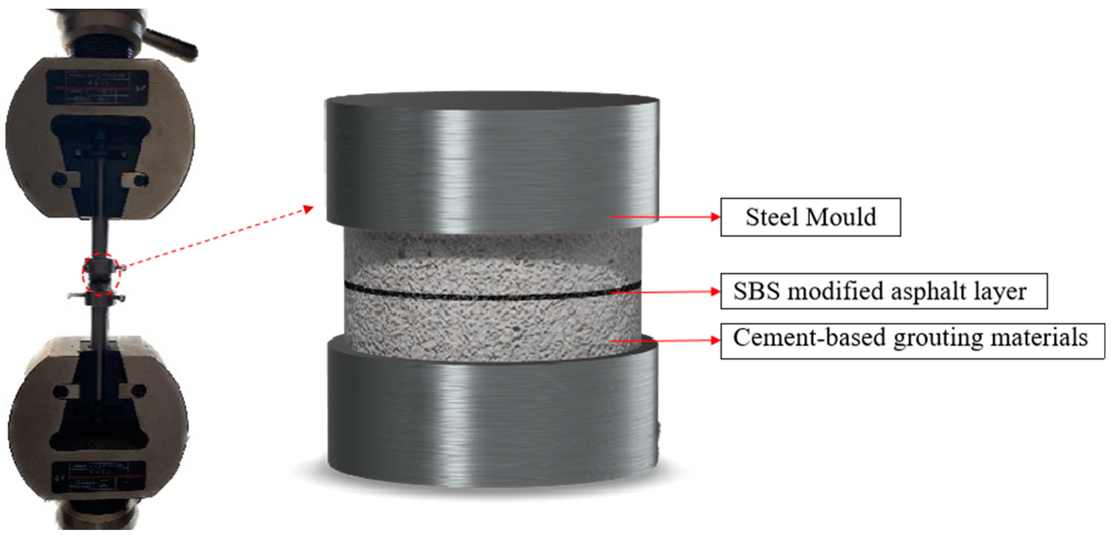
- Sample preparation: The cementitious grouting material was poured into cylindrical specimens with a diameter of 25 mm and a thickness of 15 mm. After 3 d of maintenance, a small amount of SBS asphalt was applied on the surface of the specimens. Two specimens prepared from the same cementitious grouting material were squeezed. The thickness of asphalt film was controlled at 10 (±1) μm.
- (2)
- Sample assembly: the samples prepared in (1) were fixed with two direct stretching jigs after being maintained to a specified age.
- (3)
- Test operation: The moving beam was adjusted to the appropriate position. Then, the direct tensile jig was fixed to the universal testing machine, and tensile damage was performed to the interface with a tensile speed of 10 mm/min. At least three sets of parallel tests were conducted for each interface.
3. Results and Discussion
3.1. Optimal Preparation Process
3.1.1. Orthogonal Experimental Design Method
3.1.2. Gray Correlation Analysis Method
3.1.3. Comprehensive Weighted Scoring Method
3.2. Optimal Modifiers
3.2.1. Principal Component Analysis
3.2.2. Applicability Test of Principal Component Analysis
3.2.3. Principal Component Analysis Process
3.3. Modification Mechanism Analysis
3.3.1. Mechanism for Improving the Strength of the Cement–Asphalt Interface
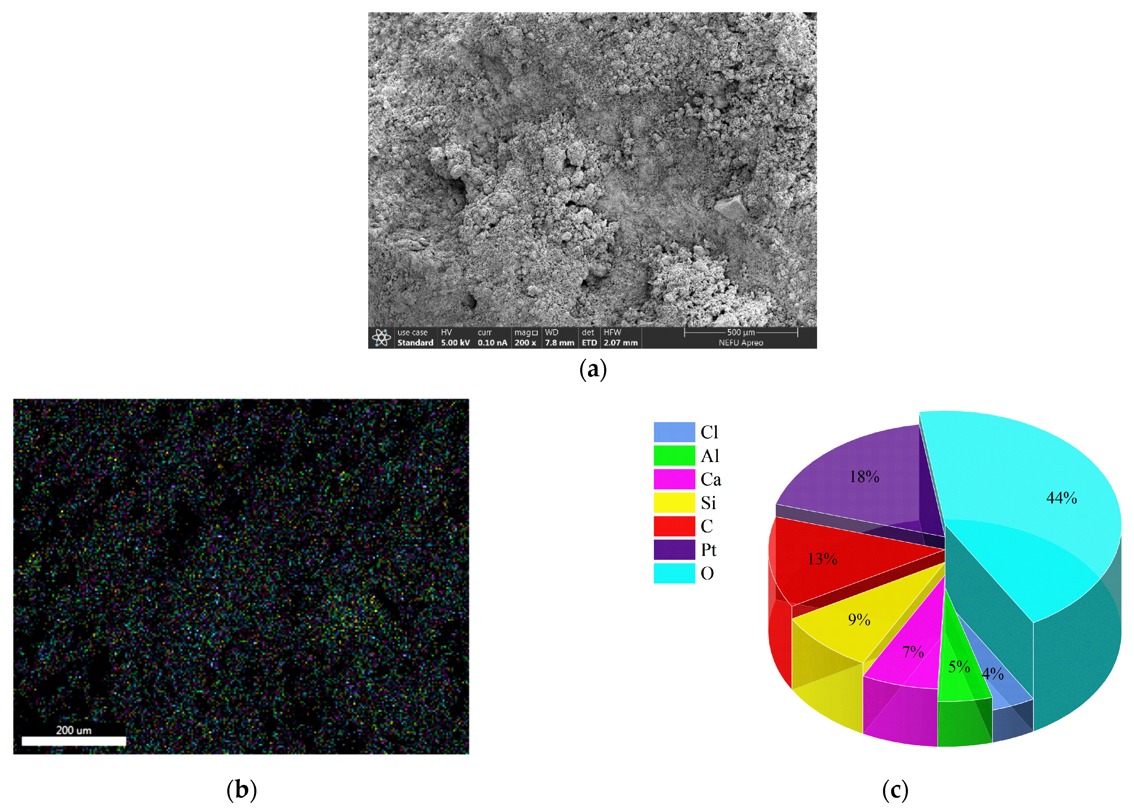
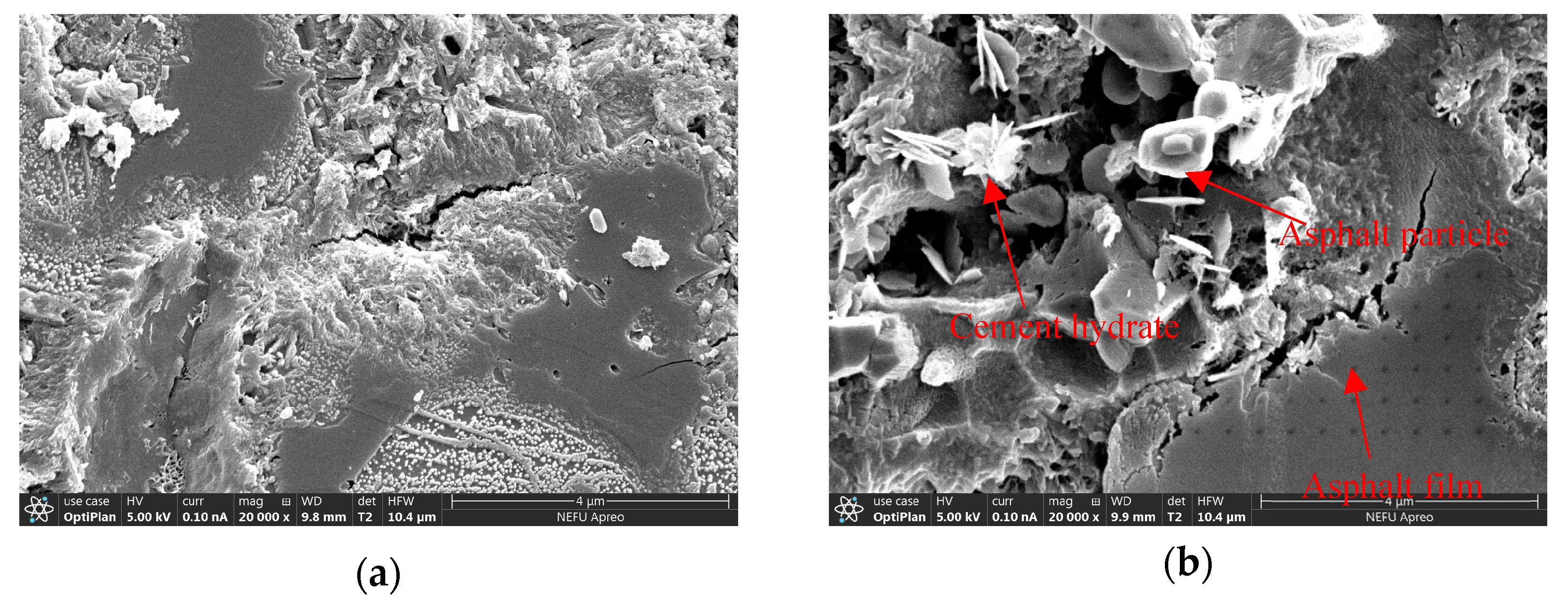
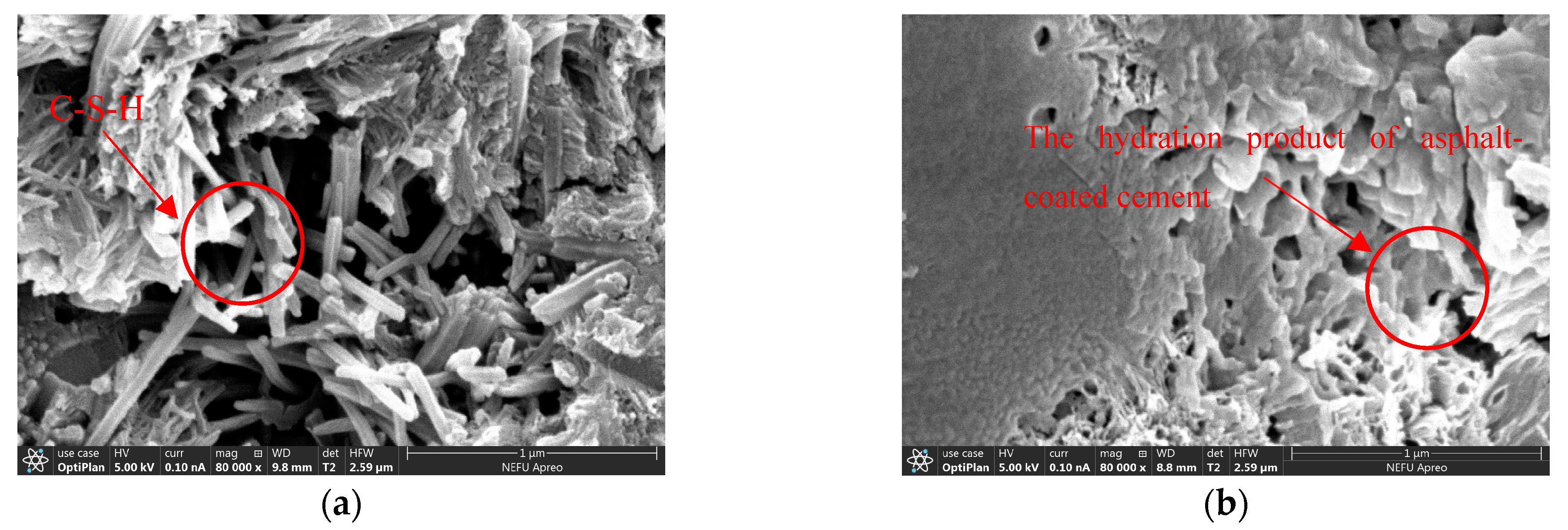
3.3.2. Microscopic Morphology and Energy Spectrum Analysis
4. Conclusions
5. Recommendation
Author Contributions
Funding
Institutional Review Board Statement
Data Availability Statement
Acknowledgments
Conflicts of Interest
References
- Wang, L.; Jun, H. Experimental Study on Improving Properties of Semi-flexible Pavement Materials with Styrene-acrylic Emulsion. J. Highw. Transp. Sci. Technol. 2021, 38, 27–32. (In Chinese) [Google Scholar] [CrossRef]
- Vavrik, W.; Carpenter, S. Calculating air voids at specified number of gyrations in superpave gyratory compactor. Transp. Res. Rec. J. Transp. Res. Board 1998, 1630, 117–125. [Google Scholar] [CrossRef]
- Polaczyk, P.; Huang, B.; Shu, X.; Gong, H. Investigation into Locking Point of Asphalt Mixtures Utilizing Superpave and Marshall Compactors. J. Mater. Civ. Eng. 2019, 31, 04019188. [Google Scholar] [CrossRef]
- Setyawan, A. Development of Semi-Flexible Heavy-Duty Pavements. Ph.D. Thesis, University of Leeds, Leeds, UK, 2006. [Google Scholar]
- Afonso, M.L.; Dinis-Almeida, M.; Pereira-de-Oliveira, L.A.; Castro-Gomes, J.; Zoorob, S.E. Development of a semi-flexible heavy duty pavement surfacing incorporating recycled and waste aggregates–Preliminary study. Constr. Build. Mater. 2016, 102, 155–161. [Google Scholar] [CrossRef]
- Ling, T.Q.; Zhao, Z.J.; Xiong, C.H.; Dong, Y.Y.; Liu, Y.Y.; Dong, Q. The Application of Semi-Flexible Pavement on Heavy Traffic Roads. Int. J. Pavement Res. Technol. 2009, 2, 211–217. [Google Scholar] [CrossRef]
- Husain, N.M.; Karim, M.R.; Mahmud, H.B.; Koting, S. Effects of Aggregate Gradation on the Physical Properties of Semiflexible Pavement. In Advances in Materials Science and Engineering; Xu, A., Ed.; Hindawi Publishing Corporation: London, UK, 2014; p. 529305. [Google Scholar] [CrossRef]
- Lu, B. French New Road Standard Structure Manual; People’s Transportation Press: Beijing, China, 1987. [Google Scholar]
- Pelland, R.J.; Gould, J.S.; Mallick, R.B. Selecting a Rut Resistant Hot Mix Asphalt for Boston-Logan International Airport. In Airfield Pavements: Challenges and New Technologies; American Society of Civil Engineers: Reston, VA, USA, 2004; pp. 390–408. [Google Scholar] [CrossRef]
- Huddleston, I.J.; Zhou, H.; Hicks, R.G. Evaluation of open-graded asphalt mixtures in oregon. HMAT Hot Mix Asphalt Technol. 1996, 1, 1–5. [Google Scholar]
- Zhang, J.; Cai, J.; Pei, J.; Li, R.; Chen, X. Formulation and performance comparison of grouting materials for semi-flexible pavement. Constr. Build. Mater. 2016, 115, 582–592. [Google Scholar] [CrossRef]
- Ding, Q.; Zhao, M.; Shen, F.; Zhang, X. Mechanical behavior and failure mechanism of recycled semi-flexible pavement material. J. Wuhan Univ. Technol. Mater. Sci. Ed. 2015, 30, 981–988. [Google Scholar] [CrossRef]
- Zhou, L. Analysis on Temperature Adaptability and Failure Pattern of Semi-Flexible Composite Pavement. Master’s Thesis, Chongqing Jiaotong University, Chongqing, China, 2016. (In Chinese). [Google Scholar]
- Yang, B.; Weng, X. The influence on the durability of semi-flexible airport pavement materials to cyclic wheel load test. Constr. Build. Mater. 2015, 98, 171–175. [Google Scholar] [CrossRef]
- Imran, M.; Usman, A. Irradiated polyethylene terephthalate and fly ash based grouts for semi-flexible pavement: Design and optimisation using response surface methodology. Int. J. Pavement Eng. 2020, 23, 2515–2530. [Google Scholar] [CrossRef]
- Hao, P.; Cheng, L.; Lin, L. Road performance of semi-flexible pavement mixes. J. Chang. Univ. (Nat. Sci. Ed.) 2003, 2, 1–6. [Google Scholar] [CrossRef]
- Husain, N.M.; Mahmud, H.B.; Karim, M.R.; Hamid, N.B.A.A. Effects of aggregate gradations on properties of grouted Macadam composite pavement. In Proceedings of the 2010 2nd International Conference on Chemical, Biological and Environmental Engineering (ICBEE), Cairo, Egypt, 2–4 November 2010. [Google Scholar]
- Chen, J.; Huang, B.; Shu, X. Air-Void Distribution Analysis of Asphalt Mixture Using Discrete Element Method. J. Mater. Civ. Eng. 2013, 25, 1375–1385. [Google Scholar] [CrossRef]
- Hu, B.; Huang, W.; Yu, J.; Xiao, Z.; Wu, K. Study on the Adhesion Performance of Asphalt-Calcium Silicate Hydrate Gel Interface in Semi-Flexible Pavement Materials Based on Molecular Dynamics. Materials 2021, 14, 4406. [Google Scholar] [CrossRef] [PubMed]
- Qu, T.; Verma, D.; Alucozai, M.; Tomar, V. Influence of interfacial interactions on deformation mechanism and interface viscosity in α-chitin–calcite interfaces. Acta Biomater. 2015, 25, 325–338. [Google Scholar] [CrossRef]
- Xu, Y.; Jiang, Y.; Xue, J.; Tong, X.; Cheng, Y. High-Performance Semi-Flexible Pavement Coating Material with the Microscopic Interface Optimization. Coatings 2020, 10, 268. [Google Scholar] [CrossRef]
- Ren, J.; Xu, Y.; Zhao, Z.; Chen, J.; Cheng, Y.; Huang, J.; Yang, C.; Wang, J. Fatigue prediction of semi-flexible composite mixture based on damage evolution. Constr. Build. Mater. 2022, 318, 126004. [Google Scholar] [CrossRef]
- Cai, X.; Huang, W.; Wu, K. Study of the Self-Healing Performance of Semi-Flexible Pavement Materials Grouted with Engineered Cementitious Composites Mortar based on a Non-Standard Test. Materials 2019, 12, 3488. [Google Scholar] [CrossRef]
- Cai, X.; Shi, C.; Chen, X.; Yang, J. Identification of damage mechanisms during splitting test on SFP at different temperatures based on acoustic emission. Constr. Build. Mater. 2021, 270, 121391. [Google Scholar] [CrossRef]
- Xing, C.; Fu, L.; Zhang, J.; Chen, X.; Yang, J. Damage analysis of semi-flexible pavement material under axial compression test based on acoustic emission technique. Constr. Build. Mater. 2020, 239, 117773. [Google Scholar] [CrossRef]
- Setyawan, A. Asessing the Compressive Strength Properties of Semi-Flexible Pavements. Procedia Eng. 2013, 54, 863–874. [Google Scholar] [CrossRef]
- Yang, Y.; Ding, Q.; Huang, C.; Huang, S.L. Research on the low-temperature Cracking Resistance of Semi-flexible Pavement with Waste Rubber Powder. In Proceedings of the Asphalt Rubber 2009 Conference, Paper Presentation. Nanjing, China, 2 November 2009. [Google Scholar]
- Wang, D.; Liang, X.; Jiang, C.; Pan, Y. Impact analysis of Carboxyl Latex on the performance of semi-flexible pavement using warm-mix technology. Constr. Build. Mater. 2018, 179, 566–575. [Google Scholar] [CrossRef]
- Liu, B.; Liang, D. Effect of mass ratio of asphalt to cement on the properties of cement modified asphalt emulsion mortar. Constr. Build. Mater. 2017, 134, 39–43. [Google Scholar] [CrossRef]
- Lu, C.; Shao, H.; Chen, N.; Jiang, J. Surface modification of polyimide fibers for high-performance composite by using oxygen plasma and silane coupling agent treatment. Text. Res. J. 2022, 92, 4899–4911. [Google Scholar] [CrossRef]
- Dong, Y. Research on High-Performance Semi-Flexible Pavement Design Parameters and Construction Processes. Master’s Thesis, Chongqing Jiaotong University, Chongqing, China, 2016. (In Chinese). [Google Scholar]
- Yan, S.; Wang, Y.; Xie, L.; Wang, X. Study on the performance of semi-flexible pavement based on different pre-grouting depths. Sino-Foreign Highw. 2019, 39, 5. (In Chinese) [Google Scholar] [CrossRef]
- Yu, J.; Eri, W.; Sun, S. Optimization of Synthesis Conditions of Indigotindisulfonate Lithium Based on Orthogonal Experimental Design Method. World J. Appl. Chem. 2020, 5, 1–5. [Google Scholar] [CrossRef]


| Technical Specifications | Test Results | Specification Requirements | Test Methods |
|---|---|---|---|
| Penetration (25 °C, 0.1 mm) | 73.8 | 60–80 | ASTM D5 |
| Softening point (°C) | 69.5 | ≥55 | ASTM D36 |
| Ductility (55 °C, cm) | 38.6 | ≥30 | ASTM D113 |
| Technical Specifications | Test Results | Test Methods | |
|---|---|---|---|
| Specific surface area | 358 | ASTM C1329 | |
| Standard consistency of cement (%) | 27.5 | AASHTO T129 | |
| Initial setting time (min) | 325 | AASHTO T131 | |
| Final setting time (min) | 412 | ||
| Flexural strength (MPa) | 3 d | 5.6 | ASTM C78/C78M |
| 28 d | 8.5 | ||
| Compressive strength (MPa) | 3 d | 22.4 | ASTM C39/C39M-12a |
| 28 d | 50.3 | ||
| Technical Specifications | Technical Requirements | Test Results |
|---|---|---|
| Appearance | Transparent liquid | Transparent liquid |
| Main content | ≥97% | 99.12 |
| Density | 0.9460–0.9560 (20 °C) | 0.951 |
| Refractive index | 1.4195–1.4205 (25 °C) | 1.42 |
| Water dispersibility | Qualified | Qualified |
| Technical Specifications | Technical Requirements | Test Results |
|---|---|---|
| Ionic charge | + 1 | |
| Residue on 1.18 mm sieve (%) | ≤0.10 | 0.06 |
| Residue content (%) | ≥50.0 | 60.0 |
| Residue solubility (%) | ≥97.5 | 99.4 |
| Residue needle penetration at 25 °C (mm) | 60.0–140.0 | 80.5 |
| Residue ductility at 15 °C (cm) | ≥40.0 | 79.6 |
| Items | Requirements | Test Results |
|---|---|---|
| Appearance | Creamy white liquid with blue light | Creamy white liquid with blue light |
| Ionic charge | - | - |
| Residue content (%) | ≥50.0 | 50 |
| pH | 6–7 | 6.4 |
| Viscosity (cps) | 1000–1200 | 1120 |
| Type | Passing (%) | |||||||
|---|---|---|---|---|---|---|---|---|
| 16.0 mm | 13.2 mm | 4.75 mm | 2.36 mm | 0.6 mm | 0.3 mm | 0.15 mm | 0.075 mm | |
| SFAC-13 | 100 | 90–100 | 10–30 | 5–22 | 4–15 | 3–12 | 3–8 | 1–6 |
| S-1 | 100 | 95 | 20 | 10.5 | 9.5 | 7.5 | 5.5 | 3.5 |
| S-2 | 100 | 95 | 20 | 13.5 | 9.5 | 7.5 | 5.5 | 3.5 |
| S-3 | 100 | 95 | 20 | 16.5 | 9.5 | 7.5 | 5.5 | 3.5 |
| Technical Specifications | Test Results | Requirements | Statute |
|---|---|---|---|
| Marshall specimen height (mm) | 63 | 63.5 ± 1.3 | ASTM D6927 |
| Marshall stability (kN) | 3.39 | ≥3 | |
| Flow value (0.1 mm) | 32.5 | 20–40 | ASTM D1559 |
| Air voids (%) | 25.8 | 20–30 | AASHTO T166 |
| Connected air voids (%) | 23.0 | ≥16.0 | |
| Leakage losses (%) | 0.5 | ≤0.8 | AASHTO T305 |
| Flying dispersion loss (%) | 13.8 | ≤15 | AASHTO T96 |
| Number | Dosage (%) | Water-to-Ash Ratio | Flow Rate (s) | Compressive Strength (MPa) | Flexural Strength (MPa) |
|---|---|---|---|---|---|
| O-SFPM | 0 | 0.50 | 10.9 | 50.3 | 8.5 |
| S-SFPM | 0.3 | 0.50 | 11.5 | 47.2 | 8.9 |
| 0.5 | 0.50 | 11.8 | 45.2 | 9.1 | |
| 0.7 | 0.50 | 12.1 | 43.5 | 8.2 | |
| C-SFPM | 5 | 0.48 | 9.8 | 48.7 | 7.9 |
| 10 | 0.46 | 11.2 | 46.3 | 7.4 | |
| 15 | 0.44 | 13.4 | 42.5 | 6.7 | |
| B-SFPM | 5 | 0.48 | 11.7 | 34.2 | 9.2 |
| 10 | 0.45 | 12.8 | 39.6 | 9.8 | |
| 15 | 0.43 | 13.5 | 37.1 | 8.9 |
| Level | Factors | |||
|---|---|---|---|---|
| Dosage (%) | Concrete Curing Time (d) | Vibration Frequency (Hz) | Vibration Time (min) | |
| 1 | 0.3 | 3 | 50 | 5 |
| 2 | 0.5 | 7 | 60 | 10 |
| 3 | 0.7 | 28 | 70 | 15 |
| Test Number | Dosage (%) | Concrete Curing Time (d) | Vibration Frequency (Hz) | Vibration Time (min) |
|---|---|---|---|---|
| 1 | 0.3 | 3 | 50 | 5 |
| 2 | 0.3 | 7 | 60 | 10 |
| 3 | 0.3 | 28 | 70 | 15 |
| 4 | 0.5 | 3 | 60 | 15 |
| 5 | 0.5 | 7 | 70 | 5 |
| 6 | 0.5 | 28 | 50 | 10 |
| 7 | 0.7 | 3 | 70 | 10 |
| 8 | 0.7 | 7 | 50 | 15 |
| 9 | 0.7 | 28 | 60 | 5 |
| Test Number | MS (kN) | DS (Times-mm−1) | ε (με) | TSR (%) |
|---|---|---|---|---|
| 1 | 14.96 | 9864.37 | 1269.55 | 79.36 |
| 2 | 19.93 | 12,607.58 | 1784.68 | 87.65 |
| 3 | 21.89 | 13,758.22 | 1824.61 | 86.96 |
| 4 | 20.11 | 14,087.23 | 1957.06 | 87.29 |
| 5 | 19.24 | 13,355.30 | 1978.39 | 89.30 |
| 6 | 22.55 | 14,328.78 | 2296.27 | 92.06 |
| 7 | 19.35 | 13,569.06 | 1826.47 | 85.14 |
| 8 | 21.30 | 13,726.63 | 2099.83 | 89.19 |
| 9 | 20.52 | 14,568.75 | 2007.40 | 92.40 |
| MS (kN) | DS (Times-mm−1) | ε (με) | TSR (%) | |
|---|---|---|---|---|
| X0 | 22.55 | 14,568.75 | 2296.27 | 92.40 |
| X1 | 14.96 | 9864.37 | 1269.55 | 79.36 |
| X2 | 19.93 | 12,607.58 | 1784.68 | 87.65 |
| X3 | 21.89 | 13,758.22 | 1824.61 | 86.96 |
| X4 | 20.11 | 14,087.23 | 1957.06 | 87.29 |
| X5 | 19.24 | 13,355.30 | 1978.39 | 89.30 |
| X6 | 22.55 | 14,328.78 | 2296.27 | 92.06 |
| X7 | 19.35 | 13,569.06 | 1826.47 | 85.14 |
| X8 | 21.30 | 13,726.63 | 2099.83 | 89.19 |
| X9 | 20.52 | 14,568.75 | 2007.40 | 92.40 |
| X0 | 1 | 1 | 1 | 1 |
|---|---|---|---|---|
| X1 | 0 | 0 | 0 | 0 |
| X2 | 0.65 | 0.58 | 0.50 | 0.64 |
| X3 | 0.91 | 0.83 | 0.54 | 0.58 |
| X4 | 0.68 | 0.90 | 0.67 | 0.61 |
| X5 | 0.56 | 0.74 | 0.69 | 0.76 |
| X6 | 1.00 | 0.95 | 1.00 | 0.97 |
| X7 | 0.58 | 0.79 | 0.54 | 0.44 |
| X8 | 0.84 | 0.82 | 0.81 | 0.75 |
| X9 | 0.73 | 1.00 | 0.72 | 1.00 |
| X1 | 1 | 1 | 1 | 1 |
| X2 | 0.35 | 0.42 | 0.5 | 0.36 |
| X3 | 0.09 | 0.17 | 0.46 | 0.42 |
| X4 | 0.32 | 0.1 | 0.33 | 0.39 |
| X5 | 0.44 | 0.26 | 0.31 | 0.24 |
| X6 | 0 | 0.05 | 0 | 0.03 |
| X7 | 0.42 | 0.21 | 0.46 | 0.56 |
| X8 | 0.16 | 0.18 | 0.19 | 0.25 |
| X9 | 0.27 | 0 | 0.28 | 0 |
| X1 | 0.33 | 0.33 | 0.33 | 0.33 |
| X2 | 0.59 | 0.54 | 0.50 | 0.58 |
| X3 | 0.85 | 0.75 | 0.52 | 0.54 |
| X4 | 0.61 | 0.83 | 0.60 | 0.56 |
| X5 | 0.53 | 0.66 | 0.62 | 0.68 |
| X6 | 1.00 | 0.91 | 1.00 | 0.94 |
| X7 | 0.54 | 0.70 | 0.52 | 0.47 |
| X8 | 0.76 | 0.74 | 0.72 | 0.67 |
| X9 | 0.65 | 1.00 | 0.64 | 1.00 |
| 0.6512 | 0.7181 | 0.6067 | 0.6419 | 2.6180 |
| Test Number | Dosage (%) | Concrete Curing Time (d) | Vibration Frequency (Hz) | Vibration Time (min) | Overall Rating |
|---|---|---|---|---|---|
| 1 | 0.3 | 3 | 50 | 5 | 3023.13 |
| 2 | 0.3 | 7 | 60 | 10 | 3898.22 |
| 3 | 0.3 | 28 | 70 | 15 | 4223.41 |
| 4 | 0.5 | 3 | 60 | 15 | 4143.98 |
| 5 | 0.5 | 7 | 70 | 5 | 4148.44 |
| 6 | 0.5 | 28 | 50 | 10 | 4490.61 |
| 7 | 0.7 | 3 | 70 | 10 | 4170.88 |
| 8 | 0.7 | 7 | 50 | 15 | 4278.91 |
| 9 | 0.7 | 28 | 60 | 5 | 4289.08 |
| Inspection Indicator | Results | Inspection Requirements | |
|---|---|---|---|
| KMO Sampling suitability quantity | 0.675 | ≥0.600 | |
| Bartlett’s sphericity test | Approximate cardinality | 230.563 | - |
| Degree of freedom | 45 | - | |
| Significance | 0.000 | ≤0.005 | |
| MS | DS | ε | TSR | |||||
|---|---|---|---|---|---|---|---|---|
| A1 | 20.03 | −1.07165 | 12,485.24 | −0.52581 | 1535.44 | −1.17119 | 85.12 | −0.93848 |
| A2 | 22.55 | 0.56505 | 14,328.78 | −0.39908 | 2296.27 | 0.74265 | 92.06 | 1.25263 |
| A3 | 23.36 | 1.09114 | 19,996.28 | 1.49602 | 2165.20 | 0.91604 | 89.18 | 0.34335 |
| A4 | 20.78 | −0.58454 | 11,826.02 | −0.57113 | 1807.24 | −0.48750 | 86.01 | −0.65749 |
| ×1 | ×2 | ×3 | ×4 | |
|---|---|---|---|---|
| ×1 | 1.000 | 0.864 | 0.924 | 0.824 |
| ×2 | 0.864 | 1.000 | 0.608 | 0.478 |
| ×3 | 0.924 | 0.608 | 1.000 | 0.955 |
| ×4 | 0.824 | 0.478 | 0.955 | 1.000 |
| Total Variance Explained | ||||||
|---|---|---|---|---|---|---|
| Ingredients | Initial Eigenvalue | Extraction of the Sum of Squares of Loads | ||||
| Total | Percentage of Variance | Cumulative (%) | Total | Percentage of Variance | Cumulative (%) | |
| 1 | 3.347 | 83.671 | 83.671 | 3.347 | 83.671 | 83.671 |
| 2 | 0.614 | 15.340 | 99.011 | 0.614 | 15.340 | 99.011 |
| 3 | 0.040 | 0.989 | 100.000 | |||
| 4 | 6.705 × 10⁻¹⁷ | 1.676 × 10⁻¹⁵ | 100.000 | |||
| Types | Principal Component Score | Principal Component Score | Overall Score Z | Ranking |
|---|---|---|---|---|
| O-SFRM | −1.9279 | 0.2446 | −1.5756 | 4 |
| S-SFPM | 1.4084 | −0.9503 | 1.0326 | 2 |
| C-SFPM | 1.7097 | 0.9127 | 1.5705 | 1 |
| B-SFPM | −1.1902 | −0.2070 | −1.0276 | 3 |
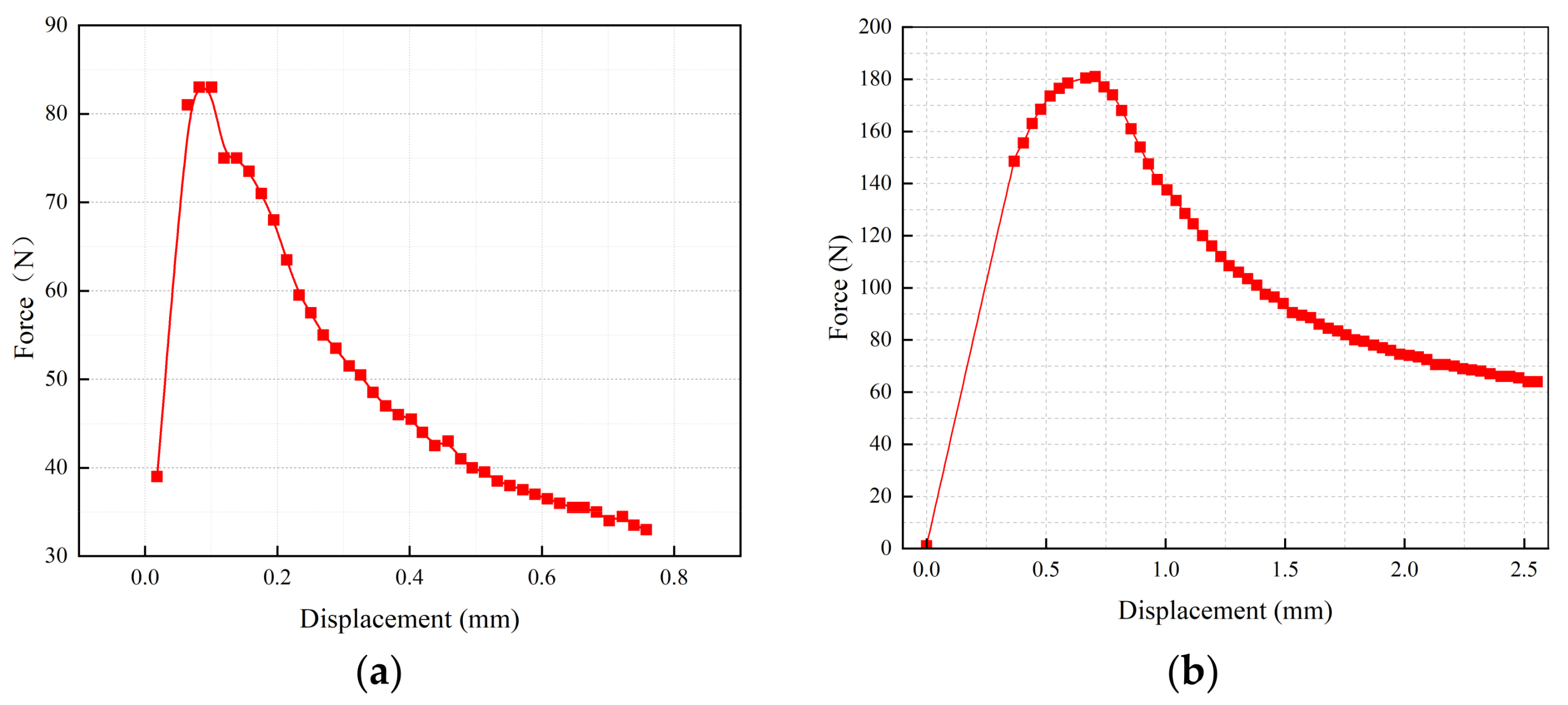
| Interface Type | Maximum Test Force (N) | Interfacial Modulus (MPa) |
|---|---|---|
| General cement-based grouting material–asphalt interface | 83.0 | 120.76 |
| Cementitious grouting material with 5% cationic emulsified asphalt—asphalt interface | 181.0 | 413.25 |
Disclaimer/Publisher’s Note: The statements, opinions and data contained in all publications are solely those of the individual author(s) and contributor(s) and not of MDPI and/or the editor(s). MDPI and/or the editor(s) disclaim responsibility for any injury to people or property resulting from any ideas, methods, instructions or products referred to in the content. |
© 2023 by the authors. Licensee MDPI, Basel, Switzerland. This article is an open access article distributed under the terms and conditions of the Creative Commons Attribution (CC BY) license (https://creativecommons.org/licenses/by/4.0/).
Share and Cite
Cheng, P.; Ma, G.; Li, Y. Preparation and Performance Improvement Mechanism Investigation of High-Performance Cementitious Grout Material for Semi-Flexible Pavement. Polymers 2023, 15, 2631. https://doi.org/10.3390/polym15122631
Cheng P, Ma G, Li Y. Preparation and Performance Improvement Mechanism Investigation of High-Performance Cementitious Grout Material for Semi-Flexible Pavement. Polymers. 2023; 15(12):2631. https://doi.org/10.3390/polym15122631
Chicago/Turabian StyleCheng, Peifeng, Guangtao Ma, and Yiming Li. 2023. "Preparation and Performance Improvement Mechanism Investigation of High-Performance Cementitious Grout Material for Semi-Flexible Pavement" Polymers 15, no. 12: 2631. https://doi.org/10.3390/polym15122631