Author Contributions
Conceptualization, L.S. and A.E.; methodology, S.Ø.R., L.S. and A.E.; software, N.P.V. and S.Ø.R.; validation, S.Ø.R., L.S. and A.E.; formal analysis, S.Ø.R. and A.E.; investigation, S.Ø.R. and A.E.; resources, L.S. and A.E.; data curation, S.Ø.R. and A.E.; writing—original draft preparation, S.Ø.R. and A.E.; writing—review and editing, S.Ø.R. and A.E.; visualization, N.P.V. and S.Ø.R.; supervision, N.P.V., L.S. and A.E.; project administration, L.S. and A.E.; funding acquisition, L.S. and A.E. All authors have read and agreed to the published version of the manuscript.
Figure 1.
A simple blade profile made from a NACA0009 profile to test the design concepts on a general structure. The lines on the blade indicate the geometrical features; they do not represent the mesh.
Figure 1.
A simple blade profile made from a NACA0009 profile to test the design concepts on a general structure. The lines on the blade indicate the geometrical features; they do not represent the mesh.
Figure 2.
The NACA blade model is viewed from the leading-edge root perspective. A NACA0009 foil-shaped cross-section at 40% blade length is highlighted in red. These different cross-sections were tracked along the blade during blade loading to observe and quantify the deformation characteristics. The red text, RP-1, indicates the reference point that with the small green text, MPC, and the yellow lines makes up the BC.
Figure 3.
Model illustrations based on the investigated design concepts: (a) a hollow aluminium blade and (b) a hollow composite blade with anisotropic surface laminates. (c) is a blade made from a solid brass leading edge as an internal structure with a hollow blade tail and (d) illustrates a solid aluminium blade with no root fixture on the blade trailing edge freeing the blade’s tail movement.
Figure 4.
The NACA blade has a square frame and a symmetric foil profile throughout the length. The propeller blade has a more complex shape; for example, a skew, changing the angle of the rotation centre through the blade-tip line. The propeller rotation direction is indicated by the solid arrow, the change in blade angle is indicated by the dotted arrow.
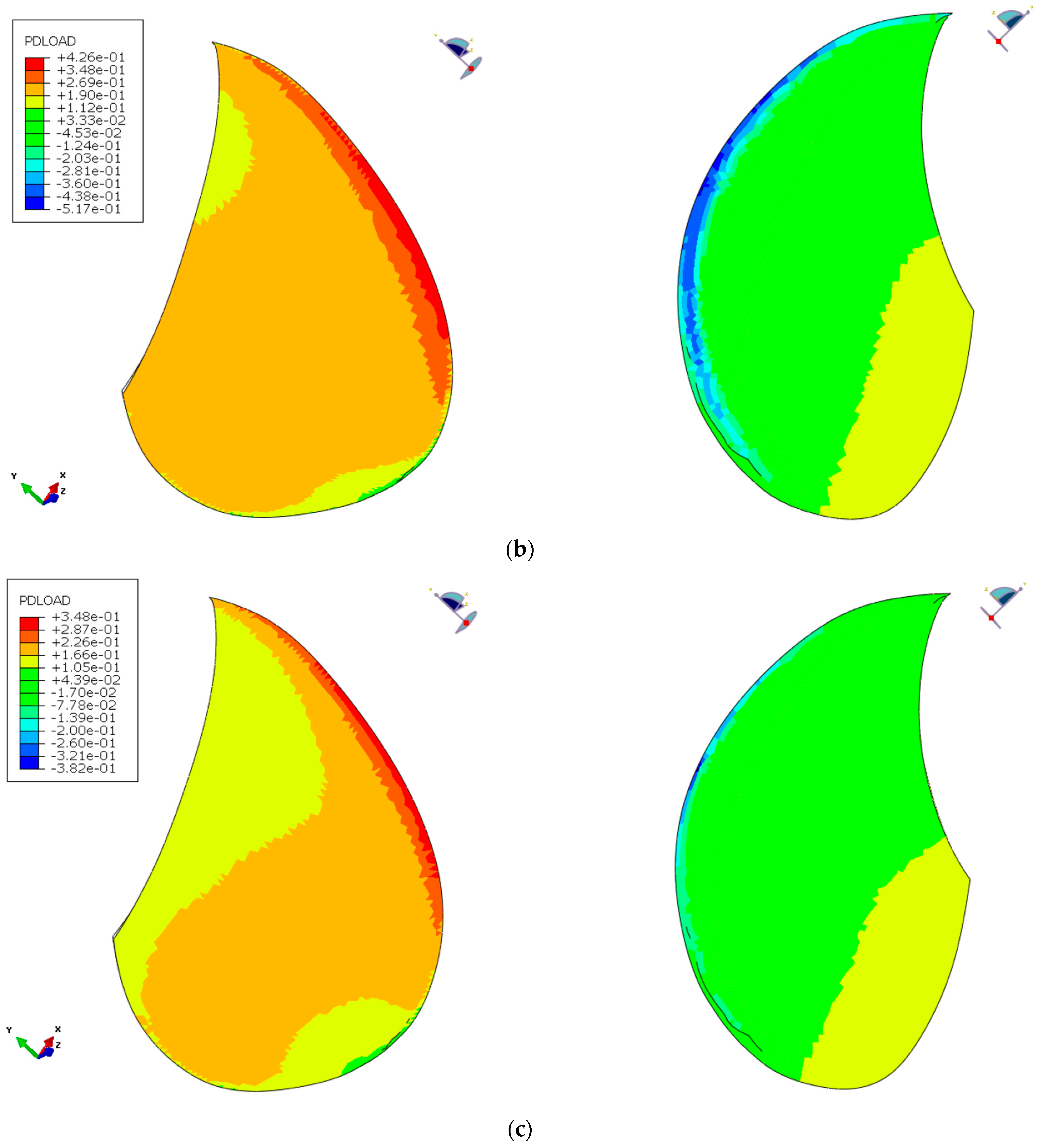
Figure 5.
(a) shows the periodic variation that should be designed for. (b,c) Illustrate the pressure distributions in the maximum load case (b) and the minimum load case (c) under periodic loading. The pressure is highest in the red and orange areas and lowest (due to suction) in the blue and light green areas, as shown in the legends.
Figure 6.
The circular lines were used for data collection to view the blade deformation characteristics. Figure from [
27].
Figure 6.
The circular lines were used for data collection to view the blade deformation characteristics. Figure from [
27].
Figure 7.
Blade displacement plots of the hollow and solid NACA blade models. The blades are viewed from the tip side, and the BC is on the far side. The graphs do not show that they are hollow but instead focus on how the models deform. The solid model (d), as expected, deforms to only a fraction of the other models. The shell model (a) is the most compliant of the hollow blade models (a–c).
Figure 8.
The foil cross-sections of the deformed and undeformed NACA beam baseline models. The cross-sections at 50%, 70% and 90% of the blade length are shown. The deflection (δ), twist (α), camber (f), chord length (C) and thickness (T) were tracked for each cross-section. The blue dotted lines are the undeformed chord lines while the orange lines are the chord line of the deformed foil.
Figure 9.
Hollow-shell models’ deformation characteristics compared to the baseline case.
Figure 9.
Hollow-shell models’ deformation characteristics compared to the baseline case.
Figure 10.
First and second models used only plies that covered the entire surface, indicated by illustration (
a). (
b) shows the third model with a local patch, a flange, on both sides of the location indicated in blue. The areas in the figure refer to
Table 2.
Figure 10.
First and second models used only plies that covered the entire surface, indicated by illustration (
a). (
b) shows the third model with a local patch, a flange, on both sides of the location indicated in blue. The areas in the figure refer to
Table 2.
Figure 11.
Comparison of the deformation characteristics of hollow anisotropic composite NACA blade models and the baseline case.
Figure 11.
Comparison of the deformation characteristics of hollow anisotropic composite NACA blade models and the baseline case.
Figure 12.
The geometry of the internal structures investigated in the NACA blade. The internal structures were made of titanium, and the hollow blade was made of aluminium. (a) was called LE-mast, (b) was LE-cornerstone and (c) was LE-framework.
Figure 12.
The geometry of the internal structures investigated in the NACA blade. The internal structures were made of titanium, and the hollow blade was made of aluminium. (a) was called LE-mast, (b) was LE-cornerstone and (c) was LE-framework.
Figure 13.
Comparison of the reinforcing-structure blade models and baseline model of a solid NACA blade.
Figure 13.
Comparison of the reinforcing-structure blade models and baseline model of a solid NACA blade.
Figure 14.
Graphic representation of how the BC was released from the tail of the NACA blade to achieve bend–twist deformation. The small green text indicates the MPC reference point.
Figure 14.
Graphic representation of how the BC was released from the tail of the NACA blade to achieve bend–twist deformation. The small green text indicates the MPC reference point.
Figure 15.
Comparison of the models that free up the tail to obtain bend–twist deformation. A solid isotropic model is plotted as the baseline.
Figure 15.
Comparison of the models that free up the tail to obtain bend–twist deformation. A solid isotropic model is plotted as the baseline.
Figure 16.
Composition of the “combined design concepts” for the proposed NACA blade design. The solid reinforcing structure was made of steel and epoxy and was used in combination with two internal FRP ribs. In addition, a hollow anisotropic FRP surface shell and FRP top and bottom end-piece caps are used. Finally, 66% of the tail was freed up. Some product development that explores assembly and fastening methods will be needed for this blade design to have a physical prototype.
Figure 17.
Global deformation contour of the combined NACA blade design in (a) and the deformation characteristics of the design at radii of 50%, 70% and 90% in (b). (c) compares the deformation characteristics between the combined NACA blade and the baseline case. The blue dotted lines are the undeformed chord lines while the orange lines are the chord line of the deformed foil.
Figure 18.
Comparison of the deformation characteristics of the solid isotropic model and the hollow isotropic models loaded with the maximum periodic load.
Figure 18.
Comparison of the deformation characteristics of the solid isotropic model and the hollow isotropic models loaded with the maximum periodic load.
Figure 19.
(a) shows the material composition in the combined propeller-blade design with the BC indicated in yellow. (b,c) shows the FEA estimation of the strain field in the blade designs’ composite surfaces and the blade’s internal substructures under maximum loading.
Figure 19.
(a) shows the material composition in the combined propeller-blade design with the BC indicated in yellow. (b,c) shows the FEA estimation of the strain field in the blade designs’ composite surfaces and the blade’s internal substructures under maximum loading.
Figure 20.
The global displacement contour of the typical propeller-blade design is shown in (a), and the deformation characteristics of the design at radii of 50%, 70% and 90% for both load cases are shown in (b). In (c), a comparison plot of the deformation characteristics of the final and baseline reference designs is shown.
Table 1.
Material properties used to model the FRP materials.
Table 1.
Material properties used to model the FRP materials.
| FRP Ply Material | E1 [MPa] | E2 [MPa] | E3 [MPa] | ν12 | ν13 | ν23 | G12 [MPa] | G13 [MPa] | G23 [MPa] | Thickness [mm] |
|---|
| CFRP Woven [0,90] | 58,000 | 58,000 | 7500 | 0.05 | 0.3 | 0.3 | 3500 | 3300 | 3300 | 0.46 |
| CFRP UD | 117,000 | 7500 | 7500 | 0.34 | 0.34 | 0.5 | 3500 | 3500 | 3300 | 0.3 |
| GFRP Woven [0,90] | 26,000 | 26,000 | 8000 | 0.1 | 0.25 | 0.25 | 3800 | 2800 | 2800 | 0.4 |
Table 2.
Layup of the anisotropic NACA models. The layup angles in dark red text are CFRP [0,90] plies, and the plies in black text are CFRP UD plies. The * indicates extra flange plies.
Table 2.
Layup of the anisotropic NACA models. The layup angles in dark red text are CFRP [0,90] plies, and the plies in black text are CFRP UD plies. The * indicates extra flange plies.
| Model | Area | No. Plies | Layup | Maximum Strain |
|---|
| Quasi-isotropic | 1 | 22 | [0,45,0…45,0,45] | 3.41% |
| Anisotropic | 2 | 26 | [0,70,30,20,30,20,70,30,20,30,20,30,0,30,0,30,20,30,20, 30,20,30,20,30,70,0] | 4.90% |
| Extra flange patch | 3 | 26 + 9* | [0,70,30,20,0*,30*,30,20,20*,70,30,30*,20,70,30,20,30,0, 70*,30,0,30,20,30,20,30*,30,20*,20,30,20,30*,0*,30,70,0] | 4.76% |
Table 3.
Laminate stack description for the composite components in
Figure 15. Only CFRP was used in this design. The layup angles in dark red text are CFRP [0,90] plies, and the plies in black text are CFRP UD plies. The * indicates extra flange plies.
Table 3.
Laminate stack description for the composite components in
Figure 15. Only CFRP was used in this design. The layup angles in dark red text are CFRP [0,90] plies, and the plies in black text are CFRP UD plies. The * indicates extra flange plies.
| Component | No. Plies | Layup |
|---|
| Anisotropic FRP laminate | 25 | [0,20,30,20,30,20,30,20,30,0,30,70,30,70,30,0,30,20,30,20,30,20,30,20,0] |
| Extra flange patch plies | 25 + 12* | [0,20,70*,30*,30,20*,20,30,20,30,30*,20,30,0,30*,0*,30,70,30,70, 30,0*,30*,0,30,20,30*,30,20,30,20,20*,30, 30*,70*,20, 0] |
| Internal rib | 22 | [0,45,0,45,0,45,30,20,60,70,0,0,70,60,20,30,45,0,45,0,45,0] |
| End-piece rib | 15 | [0,45, 0,45, 0,45, 0,45, 0,45, 0,45, 0,45, 0,45] |
Table 4.
Relative deformation characteristics for several design cases compared with the standard solid metal blade. Relative values are used because both the NACA blade geometry and the load case are arbitrary. As the values are relative to the reference case, they are unitless.
Table 4.
Relative deformation characteristics for several design cases compared with the standard solid metal blade. Relative values are used because both the NACA blade geometry and the load case are arbitrary. As the values are relative to the reference case, they are unitless.
| NACA Models | | Deflection | Twist | Twist per Deflection | Camber Change (Foil Shape) |
|---|
| | Radius | 0.5 | 0.7 | 0.9 | 0.5 | 0.7 | 0.9 | 0.5 | 0.7 | 0.9 | |
| Solid isotropic | Relative reference case | 1 | 1 | 1 | 1 | 1 | 1 | 1 | 1 | 1 | Very small |
| Hollow isotropic | Continuum shell | 4.3 | 3.5 | 2.9 | 5.3 | 4.3 | 2.6 | 1.16 | 1.15 | 0.88 | Small |
| Hollow solid | 4.4 | 3.5 | 2.9 | 4.3 | 3.8 | 2.6 | 0.96 | 1 | 0.88 | Very small |
| Shell | 4.7 | 3.8 | 3.2 | 6.6 | 5.8 | 4.2 | 1.3 | 1.4 | 1.29 | Very small |
| Anisotropic laminates | Quasi-Isotropic | 8.2 | 6.6 | 5.6 | 11.6 | 10 | 7.4 | 1.3 | 1.4 | 1.29 | Medium |
| Anisotropic | 8.8 | 7.3 | 6.3 | 20.3 | 18.8 | 16 | 2.16 | 2.3 | 2.5 | Medium |
| Anisotropic + local flange | 7.2 | 6.2 | 5.4 | 17 | 16 | 14 | 2.21 | 2.4 | 2.5 | Small |
| Reinforcing structures | LE-mast | 3.8 | 3 | 2.4 | 5.6 | 4.8 | 3.2 | 1.4 | 1.45 | 1.3 | Medium |
| Cornerstone | 2.3 | 1.6 | 1.09 | 8 | 7.3 | 5.6 | 3.2 | 4.3 | 4.9 | Medium |
| Framework | 2.4 | 1.7 | 1.16 | 7.6 | 7.3 | 5.4 | 3 | 3.9 | 4.5 | Medium |
| Solid isotropic with free tail | 50% | 1.3 | 1.2 | 1.2 | 2.3 | 2 | 1.8 | 1.6 | 1.5 | 1.35 | Very small |
| 66% | 2.3 | 2 | 1.9 | 5 | 4 | 3.4 | 2.1 | 1.9 | 1.7 | Very small |
| 75% | 3.1 | 2.7 | 2.5 | 7 | 5.5 | 4.6 | 2.17 | 1.9 | 1.8 | Very small |
| Combined design | All design concepts combined | 14.8 | 10.8 | 8.7 | 51.3 | 39.2 | 31.2 | 3.2 | 3.4 | 3.5 | Medium |
Table 5.
Laminate stack description for the composite components in
Figure 19. The layup angles in dark red text are CFRP [0,90] plies, the blue text is GFRP woven [0,90] plies, and the plies in black text are CFRP UD plies. The * indicates extra flange plies.
Table 5.
Laminate stack description for the composite components in
Figure 19. The layup angles in dark red text are CFRP [0,90] plies, the blue text is GFRP woven [0,90] plies, and the plies in black text are CFRP UD plies. The * indicates extra flange plies.
| Area | No. Plies | Layup |
|---|
| Suction side | 11 | [45,30,20,30,45,30,45,30,20,30,45] |
| Extra flange area | 15 + 4* | [45,20,10,20,10*,20*,45,20,45,20*,10*,20,10,20,45] |
| Pressure side | 15 | [−20, −30, −60, −30, −20, −30, −45, −30, −45, −30, −20, −30, −60, −30, −20] |
| FRP Bottom side | 15 | [0,45,20, −20,45,0,45,0,45,0,45, −20,20,45,0] |
Table 6.
Relative deformation characteristics for the proposed design compared to the standard hollow-solid metal blade. Because the values are relative to the reference case, they are unitless and represent the bend–twist efficiency.
Table 6.
Relative deformation characteristics for the proposed design compared to the standard hollow-solid metal blade. Because the values are relative to the reference case, they are unitless and represent the bend–twist efficiency.
| Propeller Blade Models | | Deflection | Twist | Twist per
Deflection | Camber Change |
|---|
| | radius | 0.5 | 0.7 | 0.9 | 0.5 | 0.7 | 0.9 | 0.5 | 0.7 | 0.9 | |
| Hollow-solid isotropic blade, reference case | Maximum periodic load | 1 | 1 | 1 | 1 | 1 | 1 | 1 | 1 | 1 | Small |
| Minimum periodic load | 0.55 | 0.55 | 0.54 | 0.5 | 0.55 | 0.6 | 0.88 | 1 | 1.08 | Small |
| Typical propeller blade | Maximum periodic load | 1.96 | 0.91 | 0.88 | 42.5 | 4.92 | 4.3 | 17.9 | 5.3 | 4.85 | Large |
| Minimum periodic load | 1.09 | 0.51 | 0.49 | 23 | 2.7 | 2.4 | 16.9 | 5.3 | 4.8 | Large |
Table 7.
Comparison between achieved pitch change and change in apparent angle at radii of 0.5, 0.7 and 0.9.
Table 7.
Comparison between achieved pitch change and change in apparent angle at radii of 0.5, 0.7 and 0.9.
| | R = 0.5 | R = 0.7 | R = 0.9 |
|---|
| Change in pitch | 0.41° | 0.85° | 1.52° |
| Change in inflow angle | 2.3° | 1.3° | 0.8° |
| % countered variation | 17% | 65% | 190% |
Table 8.
Deformation characteristics of the proposed propeller design under chosen load cases and the Kumar and Wurm propeller blade under cruising load.
Table 8.
Deformation characteristics of the proposed propeller design under chosen load cases and the Kumar and Wurm propeller blade under cruising load.
| Propeller-Blade Models | Deflection [mm] | Twist [°] | Twist per Deflection [°/mm] |
|---|
| radius | 0.5 | 0.7 | 0.9 | 0.5 | 0.7 | 0.9 | 0.5 | 0.7 | 0.9 |
| Kumar and Wurm design | 15 | 31 | 47 | 0.5 | 1.3 | 2.3 | 0.03 | 0.04 | 0.05 |
| Proposed design under minimum load | 2.6 | 5.5 | 10 | 0.5 | 1.0 | 1.8 | 0.19 | 0.18 | 0.18 |
| Proposed design under maximum load | 4.7 | 10 | 18.6 | 0.9 | 1.8 | 3.3 | 0.19 | 0.18 | 0.18 |


