Article

Diffusion-Enhanced Förster Resonance Energy Transfer in Flexible Peptides: From the Haas-Steinberg Partial Differential Equation to a Closed Analytical Expression

School of Science, Constructor University, 28759 Bremen, Germany
*
Authors to whom correspondence should be addressed.
Polymers 2023, 15(3), 705; https://doi.org/10.3390/polym15030705
Submission received: 19 December 2022 / Revised: 20 January 2023 / Accepted: 23 January 2023 / Published: 30 January 2023

Abstract

:
In the huge field of polymer structure and dynamics, including intrinsically disordered peptides, protein folding, and enzyme activity, many questions remain that cannot be answered by methodology based on artificial intelligence, X-ray, or NMR spectroscopy but maybe by fluorescence spectroscopy. The theory of Förster resonance energy transfer (FRET) describes how an optically excited fluorophore transfers its excitation energy through space to an acceptor moiety—with a rate that depends on the distance between donor and acceptor. When the donor and acceptor moiety are conjugated to different sites of a flexible peptide chain or any other linear polymer, the pair could in principle report on chain structure and dynamics, on the site-to-site distance distribution, and on the diffusion coefficient of mutual site-to-site motion of the peptide chain. However, the dependence of FRET on distance distribution and diffusion is not defined by a closed analytical expression but by a partial differential equation (PDE), by the Haas-Steinberg equation (HSE), which can only be solved by time-consuming numerical methods. As a second complication, time-resolved FRET measurements have thus far been deemed necessary. As a third complication, the evaluation requires a computationally demanding but indispensable global analysis of an extended experimental data set. These requirements have made the method accessible to only a few experts. Here, we show how the Haas-Steinberg equation leads to a closed analytical expression (CAE), the Haas-Steinberg-Jacob equation (HSJE), which relates a diffusion-diagnosing parameter, the effective donor–acceptor distance, to the augmented diffusion coefficient, J, composed of the diffusion coefficient, D, and the photophysical parameters that characterize the used FRET method. The effective donor–acceptor distance is easily retrieved either through time-resolved or steady-state fluorescence measurements. Any global fit can now be performed in seconds and minimizes the sum-of-square difference between the experimental values of the effective distance and the values obtained from the HSJE. In summary, the HSJE can give a decisive advantage in applying the speed and sensitivity of FRET spectroscopy to standing questions of polymer structure and dynamics.

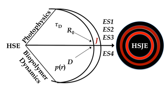
Graphical Abstract

1. Introduction

There is no question about the significance of fluorescence in multiple molecular investigations; its speed and sensitivity even enable investigations on the level of the single molecule [1]. There is also no question about the significance of Förster resonance energy transfer in structural and dynamic molecular studies as the number of citations to Förster’s original paper approaches 10,000 [2]. We believe that diffusion-enhanced fluorescence resonance energy transfer, or DFRET, on the molecule ensemble can also develop into an influential method but is, as of now, difficult to handle and non-transparent in terms of data acquisition and analytics [3,4,5,6,7,8,9,10,11,12,13,14]. This article aims to make DFRET accessible to any scientist working in one of the many fields of polymer structure and dynamics. Here, we would like to point out that the Supporting Information file we have created contains assisting information in regard to different audiences: the layman, the expert, and, especially, the scientist who wants to put our method to work.
When a protein or peptide, or any molecule, has been modified at two sites with two fluorophoric moieties, one moiety can act as FRET donor and the other as FRET acceptor. When the intermittent chain between these sites is flexible, the optically excited donor and the acceptor can approach each other by diffusional motion. In accordance with Förster’s law (Equation (1)), the probability of energy transfer from donor to acceptor increases. Förster’s law connects the distance-dependent transfer rate constant, kT(r), with the rate constant of deactivation in the donor-only peptide, kD, with the Förster distance, R0, a constant that characterizes the donor-acceptor pair, and with the donor–acceptor distance, RDA.
k T = k D ( R 0 R DA ) 6
Figure 1 gives a survey of the processes relevant in DFRET.
After excitation, the excited donor (D) can become deactivated in one of three ways: by emitting fluorescence with the rate constant krad (“kradiative”); by being quenched, for instance by iodine ions, with the rate constant knrad (“knon-radiative”); or by transferring its excitation energy to the acceptor (A) with the rate constant kFRET. In experimental measurements, we always use the donor-acceptor peptide (the DA-peptide) together with the “donor-only” peptide (the D-peptide). If no acceptor is present but only the donor, the measured rate of deactivation is kD = krad + knrad (Figure 1; (I)). In the donor-acceptor peptide, in presence of an acceptor, the measured rate is kDA = krad + knrad + kFRET (Figure 1, (II)). Subtracting (I) from (II) yields the effective FRET rate, kFRET, kFRET = kDAkD (Equation (2)). In any normal situation, kFRET increases with increasing diffusional motion between donor and acceptor. During the lifetime of the donor fluorescence, donor and acceptor can approach each other, and the probability of the FRET event increases in accordance with Förster’s law (Equation (1)), where kT is the distance-dependent Förster transfer rate constant at a specific donor–acceptor distance, RDA. Consequently, kFRET increases with diffusion, and the effective distance derived from kFRET (Figure 1, (III), (IV), Equations (3) and (4)) decreases. In summary, the effective distance (Equation (4)) is a suitable diagnostic parameter to measure the diffusion enhancement of FRET. The effective distance serves as the interface between experiment and theory, that is, between the experimental results and the numerical solutions of the Haas-Steinberg equation (HSE). To restate, the effective distance is obtained experimentally from steady-state or time-resolved measurements on the peptide equipped with donor and acceptor, the “DA-peptide” (see Figure 1), and the peptide equipped only with the donor, the “D-peptide”. Measurements on the DA-peptide yield the fluorescence intensity, IDA, in steady-state experiments or the fluorescence decay rate, kDA, in time-resolved experiments, while measurements on the D-peptide yield ID or kD. Exemplary chemical structures (Figure S1) and kinetics (Figure S2a,b) are given in the Supporting Information, Chapter 3.
k FRET = k DA k D
k FRET = k D ( R 0 R eff ) 6
R eff = k D ( R 0 k FRET ) 1 / 6

Introduction to the Haas-Steinberg Equation

The story of diffusion-enhanced FRET or DFRET started 40 years ago [3]. Since then, the number of published articles based on DFRET has remained small, not for lack of interest but for the method’s complexity [4,5,6,8,10,11,12,13,14]. In 1978, Steinberg derived what we began to call the Haas-Steinberg equation (HSE) [3]. Haas and co-workers developed unique techniques and used the HSE to tackle fundamental biological questions in protein folding, enzyme activity, and, more recently, in regard to intrinsically disordered peptides [3,5,10,11,15].
The HSE allows the calculation of theoretical effective distances. These theoretical or predicted values of HSE-based effective distances can then be fitted to the experimentally observed values in a multivariate analysis; in a global fit, that yields structure, i.e., the distance distribution, p(r), as well as dynamics, i.e., the diffusion coefficient, D.
In this work, we show how the HSE leads to a closed analytical equation, the HSJE (Haas-Steinberg-Jacob equation) by going through four equivalence statements (ES1-4). The HSJE eases and accelerates any global analysis, and, in addition, provides insight into the role of each parameter participating in DFRET.

2. Materials and Methods

The HSE was solved numerically by using the finite element method implemented in the PDE toolbox of MATLAB 2020 (MathWorks). The results from MATLAB calculations were analyzed within MATLAB 2020 and Microsoft Excel (Mac 2011). Figures were produced by using ProFit (QuantumSoft). For the global fits based on the HSJE and presented in the Supporting Information, Chapter 8, Figures S6 and S7, we used Microsoft Excel and its Solver add-in.

2.1. The HSE

The HSE can be written in various ways; we have specifically chosen the version shown in Equation (5).
N ( r , t ) t = 1 τ D N ( r , t ) 1 τ D R 0 6 r 6 N ( r , t ) + r ( N 0 ( r ) D ( N / N 0 ) r )
In Equation (5), we focus on the donor fluorescence lifetime, τD, instead of the donor deactivation rate constant, kD, used in Figure 1 (Equation (I): kD = krad + knrad). It is much easier to recall the value of a lifetime, for instance, 100 ns, than that of a rate constant, for instance, 0.01 ns−1. The donor lifetime in the donor-only peptide, τD, is simply the inverse of the rate constant, kD, in this peptide (Equation (6)).
τ D = k D 1
Our shorthand notation for the HSE will simply be “(0) = (1) + (2) + (3)”, which enables us to address the left-hand-side term of the equation with term-(0) and the right-hand-side terms of the equation with terms-(1), -(2), and -(3). The function, N(r,t), on the left-hand side is a measure of the number of chains with excited donor after donor excitation. At a specific donor–acceptor distance, r, this number decreases with time, t. Thus, we have two independent variables, r and t, and, therefore, a partial differential equation, a PDE. N(r,t) is further normalized in a way that N0 = N(r, t = 0) in term-(3) is the initial probability density distance distribution. Upon irradiation, donors become activated with a probability assumed to be random, to be independent of the presence of an acceptor at various distances. In consequence, N0 is identical to the equilibrium distance distribution, p(r), of all chains present in the measurement sample. This distance distribution, p(r), as well as the site-to-site diffusion coefficient, D, in term-(3), is what we are interested in. They inform us on the structure and the dynamics of the (bio)polymer under investigation.
In summary, the HSE is a linear partial differential equation of second order: The second derivative becomes better visible on expansion of term-(3). Further, the HSE has constant coefficients that include the parameters, D, τD, and R0. The HSE relates the rate of donor deactivation, term-(0); to the rate of donor deactivation in the absence of FRET, term-(1); plus the additional rate due to FRET, term-(2); plus the additional rate due to diffusion enhanced FRET, term-(3). A numerically obtained solution of the HSE yields the value of the effective distance between donor and acceptor. We elaborate on this calculation in Supporting Information, Chapter 4, Figure S3a–i.

2.2. Steinberg’s Derivation

Steinberg’s derivation of the HSE led him first to the following form (Equation (7)) [3].
N ( r , t ) t = k D N ( r , t ) k D R 0 6 r 6 N ( r , t ) + r ( N 0 ( r ) D ( N / N 0 ) r )
Here, the diffusion coefficient, D, in term-(3) does not depend on time, t, but it could still depend on the donor–acceptor distance, r: D = f(r). It is, however, even today, challenging to gather sufficient experimental results to investigate this possible dependence. Steinberg was content with an average diffusion coefficient that can be regarded as a constant. Then, D can be written in front of term-(3) (Equation (8)).
N ( r , t ) t = k D N ( r , t ) k D ( R 0 r ) 6 N ( r , t ) + D r ( N 0 ( r ) ( N / N 0 ) r )
When we apply Equation (6), we again obtain the HSE in the form of Equation (5). In summary, we know how to obtain Reff from experiments as well as from numerically solving the HSE. We can therefore use the HSE to globally fit the experimental data. This was quite arduous in the past, where the HSE served a bit as a black box [5,6,10,11,12,13,14]. In the Results Section, we develop the Haas-Steinberg–Jacob equation (HSJE), a closed analytical expression (CAE). Any global fit based not on the HSE (PDE) but on the HSJE (CAE) is faster by about two orders of magnitude.

3. Results

3.1. Ideas and Concepts

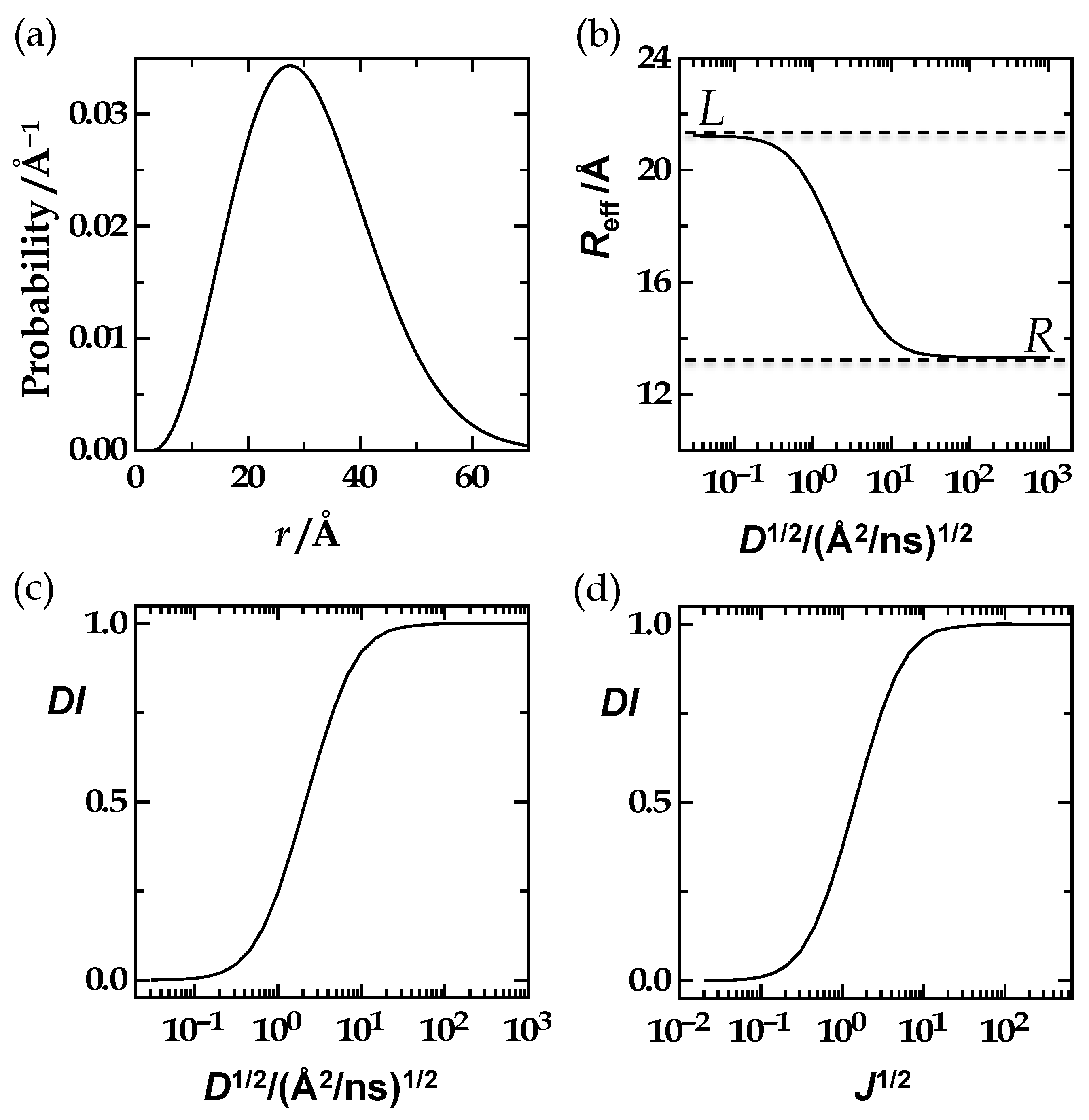
We first outline the basic ideas and concepts. Based on a freely selected distance distribution (Figure 2a) and selected values for the donor lifetime and Förster distance, τD and R0, we solved the HSE for a large range of values of the diffusion coefficient reaching from 10−3 to 106 Å2/ns. The obtained effective-distance values formed a full diffusion profile, ranging from the “static limit” in the near absence of diffusion to the “dynamic limit” at high diffusion. In figures and graphs, we always plotted the effective distance against the square root of the diffusion coefficient or, later, against the square root of the “augmented diffusion coefficient” to keep the x-axis numbers or labels manageably small and readable (Figure 2b).
We have analytical equations for both extremes of the diffusion influence (Equations (9) and (10)): The “left” value, L, of the effective distance marks the static limit or the case of no diffusion (Equation (9)), as we first derived in the Supporting Information of reference [12]. The “right” value, R, of the effective distance marks the dynamic limit or the case of infinite diffusion (Equation (10)) [12,16] The derivations of the L- and R-equations can be found in this article’s Supporting Information, Chapters 4 and 4a,b. Explanations of the two underlying basic concepts, “the Energy Transfer Efficiency” and “the Average”, can be found in in the Supporting Information, Chapters 3 and 3a,b. At first glance, these equations appear to be quite complex, but, because of their analytical character, L and R are calculated within Matlab or Excel in a fraction of a second. We note that L is a function of the Förster radius and the distance distribution, while R is a function of only the distance distribution. Further, we note that any integration of p(r) takes place from the left-integration limit, rL, to the right-integration limit, rR. A physical but oversimplified perspective is to view rL as the closest possible distance between donor and acceptor.
L = R eff , D 0 = R 0 ( ( 1 r L r R p ( r ) ( r 6 r 6 + R 0 6 ) d r ) 1 1 ) 1 / 6
R = R eff , D = r 6 1 / 6 = ( r L r R ( 1 / r 6 ) p ( r ) d r ) 1 / 6
As we have these analytical equations for the static and dynamic limit of the effective distance, the L and R values are supposed to be extremely close to the effective-distance values at the start and end of the numerically obtained diffusion profile (Figure 2b). This demands virtual identity of the analytically and numerically obtained values that always served as the first important control indicating that the numerical simulations were properly executed. We now use the L- and R-values to normalize the diffusion profiles: Equation (11) defines the diffusion influence DI. It goes from 0 or 0%, when Reff approaches L, to 1 or 100%, when Reff approaches R (Figure 2c). Thus, we distinguish in Figure 2 between the diffusion profiles, the Reff(D) or Reff(D1/2) profiles (Figure 2b), and the diffusion-influence profiles, the DI(D) or DI(D1/2) profiles (Figure 2c), or the DI(J), DI(J1/2), or DI(X) profiles (Figure 2d) after we discovered that the decisive independent variable, the decisive x-variable, is not D but J or its square root, X (Equation (12)).
D I = R eff L R L
In our quest for the HSJE, for an analytic equation that captures all possible diffusion profiles, we systematically varied the initial distance distribution as well as all coefficients of the HSE. Doing that, we found that, as mentioned, the appropriate independent variable is not the diffusion coefficient, D, but what we now call the augmented diffusion coefficient, J, composed of three coefficients: the diffusion coefficient, the donor lifetime, and the Förster radius (Equation (12)). Remarkably, J is dimensionless. To repeat, we address plots of DI versus J or its square root, X = J1/2, as diffusion-influence profiles, as DI, DI(J), or DI(X) profiles.
J = D τ D R 0 2 ;   X = J = D τ D R 0
We found that all DI-profiles are sigmoids that can be fitted to Equation (13), where X0 = J1/2. The value X0 is the X value where DI = 50%; the M value describes the steepness of the sigmoid.
D I ( X ) = ( X / X 0 ) M 1 + ( X / X 0 ) M
The sigmoidal profiles obtained from the HSE solutions appear to be perfectly point symmetrical around the point (X0, 50%) provided that a logarithmic scale is chosen for the x-axes or, equivalently, that DI is plotted against lnX. The numerically obtained profiles could then be perfectly fitted according to Equation (13). Thus, we are convinced that any DI profile follows a symmetrical sigmoid in accordance with Equation (13). This requirement of sigmoidal symmetry served as the second important control that indicates correctly performed numerical simulations. Equations (12) and (13), in combination, yield Equation (14), a first raw form of the HSJE.
In the course of our investigation, we discovered and formulated four equivalence statements that led us from D as the independent variable in the diffusion profiles, to J or its square root, X, as independent variables in the diffusion-influence profiles. We learned that the parameters X0 and M in Equation (13) are functions of just a single variable, of the ratio of the Förster radius and the left-integration limit, of R0/rL. Thus, in the last step, we completed the HSJE by numerical work to determine how X0 and M depend on R0/rL.
R eff = ( X / X 0 ) M 1 + ( X / X 0 ) M ( R L ) + L

3.2. The Equivalence Statements

In the following, we always compare effective-distance and diffusion-influence values and profiles obtained from the HSE used with two different sets of inputs that we distinguish by (1) and (2) as superscript. That is, we compare HSE(1) and HSE(2), where HSE(1) uses set(1) that consists of the distance distribution, p(1)(r), and the values, D(1), τD(1), R0(1), and rL(1), while HSE(2) uses set(2) that consists of the distance distribution, p(2)(r), and the values, D(2), τD(2), R0(2), and rL(2). Accordingly, the augmented diffusion coefficient J(1) equals D(1)τD(1)/(R0(1))2 and J(2) equals D(2)τD(2)/(R0(2))2. We also have to distinguish between the two diffusion-influence profiles obtained from HSE(1) and HSE(2), between DI(1) and DI(2) as functions of J or X, as they usually stem from different distance distributions, p(1)(r) and p(2)(r), that usually come with different L- and R-values, L(1) and R(1) and L(2) and R(2) (see Equations (9)–(11)).

3.2.1. The First Equivalence Statement: Variation of the Distance Distribution

To expose what happens if we only vary the distance distribution, we have chosen the three distributions shown in Figure 3a. The diffusion profiles that correspond to these distributions and to the chosen photophysical parameters are given in Figure 3b. These profiles are expectedly very different because any specific distance distribution comes with specific L- and R-values (Equations (9) and (10)). However, when we calculate the DI-values by using the L- and R-values characteristic for each distribution (Equation (11)), and normalize the profiles that way, we obtain perfect overlap of the resulting diffusion-influence profiles (Figure 3c). This normalization, the introduction of the diffusion-influence or DI-value defined by Equation 11 opened our path towards the HSJE.
We now express the first equivalence statement (ES1) as text and, then, in formula.

Equivalence Statement 1 (ES1, Text)

“The diffusion-influence profiles of any two well-behaved probability distributions, p(1)(r) and p(2)(r), coincide if they were obtained with the same values of the donor lifetime, τD, the Förster radius, R0, and the left-integration limit, rL.”
ES1 (formal):
For   any   p ( 1 ) ( r )   and   p ( 2 ) ( r ) :   If   D ( 1 ) = D ( 2 ) ,   τ D ( 1 ) = τ D ( 2 ) ,   R 0 ( 1 ) = R 0 ( 2 ) ,   and   r L ( 1 ) = r L ( 2 ) then   D I ( 1 ) ( J ( 1 ) ) = D I ( 2 ) ( J ( 2 ) )
Here and in the three following statements, we always use the augmented diffusion coefficient, J, defined by Equation (12), as the independent variable in diffusion-influence or DI profiles. In this first statement, J(1) and J(2) are obviously identical, and using J as the independent variable makes no difference versus using D instead, but it fosters the formal parallelism of the four equivalence statements. Two questions arise:
1.
Why do we demand that rL(1) = rL(2)? Why can ES1 not be applied if the left-integration limit differs in both sets?
In case of a smaller left-integration value, the contribution of diffusion to FRET at infinite diffusion is higher. This can be concluded from term-(2) of the HSE (Equation (5)) that encompasses Förster’s law (Equation (1)): At smaller rL values, FRET becomes faster. As a consequence, higher values of the augmented diffusion coefficient are necessary to reach the dynamic limit in the diffusion-influence profiles. Therefore, the distribution with smaller rL will lead to a diffusion-influence profile that only later reaches DI values close to 100%. This is further detailed and illustrated in the Supporting Information, Chapter 7b, Figure S4a–c.
2.
Is ES1 valid for any distance distribution equation or model? Or is it only valid for “well-behaved” models?
Prominent model equations that have been chosen in the past to describe end-to-end distance distributions in flexible peptides have been the one-parameter ideal-chain or random-coil model (Equation (16), parameter b) or the two-parameter 3D-Gaussian or skewed-Gaussian model (Equation (17), parameters a and b). The normalization constant, N, is determined through the normalization condition: The integral over p(r) from left to right integration limit has to be unity (see the Supporting Information, Chapter 7c, Equation (S26)).
p ( r ) = N r 2 ( 3 2 π b 2 ) exp ( 3 r 2 2 b 2 ) ;   b = r 2 1 / 2
p ( r ) = N r 2 exp ( a ( b r 2 ) )
Using Equations (16) or (17), we discovered that sometimes the DI-overlap of the profiles of two such distributions became less perfect in case of large discontinuities of the distributions at the point r = rL, that is, in the case of large jumps of probability-density values from zero to finite values at this point (Supporting Information, Chapter 7c, Figure S5a). In the transition region of the sigmoidal DI-profiles of two such distributions, the DI-value disagreement can become as large as 10%, undermining our efforts to develop a closed analytic equation with precisely determined constants, the HSJE. Further, such discontinuities can hardly be justified by any physical reasoning. This problem was resolved, and complete overlap was restored for all cases when we modified the distribution equations to display continuity of probability-density values at and around r = rL (Equations (18) and (19)), (Supporting Information, Chapter 7c, Figure S5b). Thus, we proceeded by using only “well-behaved” distribution equations that, by their very nature, guarantee that p(r = rL) = 0 and guarantee p(r)-value continuity (Equations (18) and (19)).
p ( r ) = N r 0 2 ( 3 2 π b 2 ) exp ( 3 r 0 2 2 b 2 ) ;   r 0 = r r L
p ( r ) = N r 0 2 exp ( a ( b r 0 2 ) ) ;   r 0 = r r L

3.2.2. The Second Equivalence Statement: Variation of the Donor Lifetime

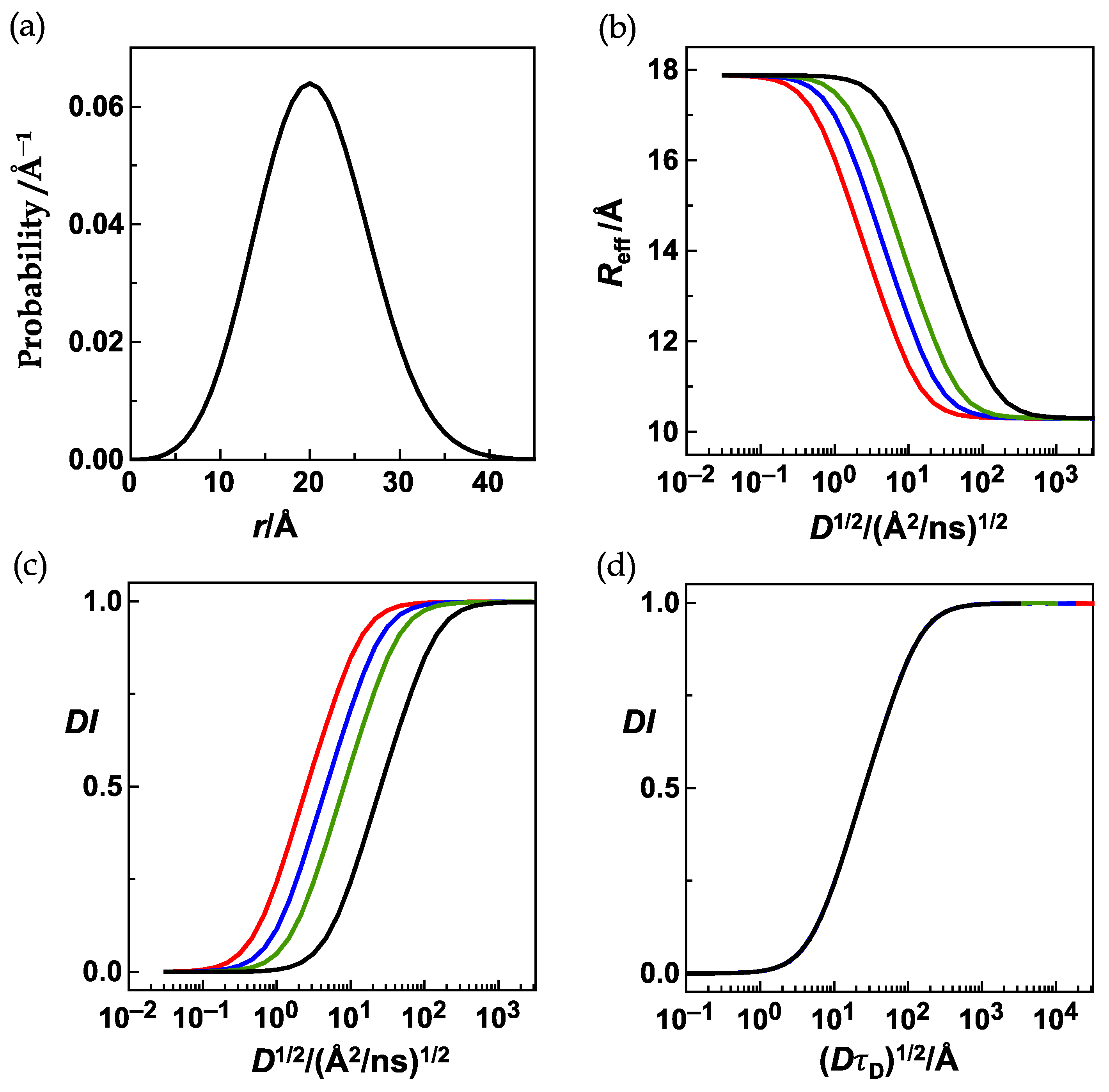
Next, we vary the donor lifetime. Figure 4a shows an exemplary distance distribution, and Figure 4b the four diffusion profiles that were obtained for this distribution and for the four donor lifetime values, 100 ns (red curve, left), 30 ns (blue curve), 10 ns (green curve), and 1 ns (black curve, right). All other parameters of the HSE were kept constant. Using the same color code, Figure 4c shows the corresponding diffusion-influence profiles. When we now plot, for each profile, the diffusion-influence value against the product of the diffusion coefficient and the corresponding donor lifetime, 100, 30, 10, or 1 ns, or against the square root of this product, we observe that the four profiles become identical (Figure 4d). Going from the diffusion coefficient, D, to the product DτD as the independent variable in diffusion-influence plots is the first of two steps towards the augmented diffusion coefficient, J.
This observed profile identity means that the values of the effective distance obtained from the HSE with input sets, set(1) and set(2), that only differ by the diffusion coefficient, D(1) in contrast to D(2), and by the donor lifetime, τD(1) in contrast to τD(2), are identical as long as the product DτD does not change, that is, as long as it is valid that D(1)τD(1) = D(2)τD(2). We now formulate the second equivalence statement and prove it to be a mathematical consequence of the HSE.

Equivalence Statement 2 (ES2, Text)

“Given any probability distribution: If the diffusion coefficient is varied from D(1) to D(2) and the donor lifetime from τD(1) to τD(2), but the product of diffusion coefficient and donor lifetime remains constant, then the diffusion-influence values obtained from the diffusion-influence functions, DI(1)(J(1)) and DI(2)(J(2)), are identical. The corresponding diffusion-influence profiles coincide”.
ES2 (formal):
For   any   p ( 1 ) ( r ) = p ( 2 ) ( r ) :   If   D ( 1 ) τ D ( 1 ) = D ( 2 ) τ D ( 2 ) ,   R 0 ( 1 ) = R 0 ( 2 ) ,   and   r L ( 1 ) = r L ( 2 ) then   D I ( 1 ) ( J ( 1 ) ) = D I ( 2 ) ( J ( 2 ) )
ES2 can be derived in several ways from the HSE (Equation (5)), as detailed in the Supporting Information, Chapter 7d.
Here we opted for a change-of-variable approach applied to the HSE (Equation (5)). We use the fact that any rescaling of time can impossibly affect the value of the effective distance (see Supporting Information, Chapter 7d). We rescale the time with the donor lifetime (Equation (21)) and insert the resulting substitutions into the HSE to arrive at Equation (22) that simplifies to Equation (23).
z = t τ D     z = t τ D     t = τ D z
1 τ D N ( r , z ) t = 1 τ D N ( r , z ) 1 τ D R 0 6 r 6 N ( r , z ) + D r ( N 0 ( r ) ( N / N 0 ) r )
N ( r , z ) z = N ( r , z ) R 0 6 r 6 N ( r , z ) + D τ D r ( N 0 ( r ) ( N / N 0 ) r )
We observe that the product of diffusion coefficient and donor lifetime, DτD, appears in the rescaled HSE (Equation (23)) at the same place as D does in the initial HSE (Equation (5)). Secondly, neither D nor τD appear at any other place of the rescaled HSE (Equation (23)). It is obvious from Equation (23) that any change of the diffusion coefficient and donor lifetime will not change the resulting effective distance, Reff, if their product, DτD, does not change. This is what ES2 expresses.

3.2.3. The Third Equivalence Statement: Variation of the Förster Radius and Left-Integration Limit

In the next step, we only change the Förster radius from R0(1) to R0(2) and the left-integration value from rL(1) to rL(2). We observe total overlap of the resulting diffusion-influence profiles, DI(1)(J(1)) and DI(2)(J(2)), if the third equivalence statement is obeyed:

Equivalence Statement 3 (ES3, Text)

“Given any probability distribution: If the Förster radius and the left-integration limit are varied but not their ratio, then the diffusion-influence values obtained from the diffusion-influence functions, DI(1)(J(1)) and DI(2)(J(2)), are identical. The corresponding diffusion-influence profiles coincide”.
ES3 (formal):
For   any   p ( 1 ) ( r ) = p ( 2 ) ( r ) :   If   D ( 1 ) τ D ( 1 ) ( R 0 ( 1 ) ) 2 = D ( 2 ) τ D ( 2 ) ( R 0 ( 2 ) ) 2   and   R 0 ( 1 ) r L ( 1 ) = R 0 ( 2 ) r L ( 2 ) then   D I ( 1 ) ( J ( 1 ) ) = D I ( 2 ) ( J ( 2 ) )
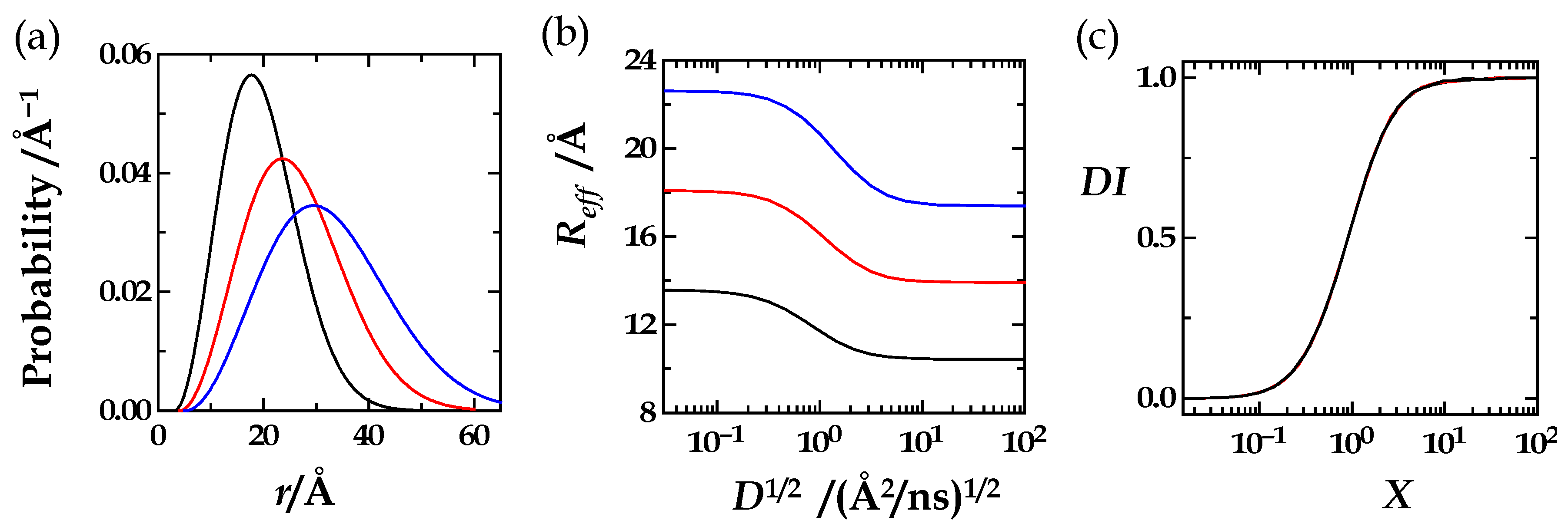
That ES3 holds true with excellent precision is illustrated in Figure 5. Here, we also tested ES1 again: We compared three different distance distributions and their DI-profiles obtained with three different pairs of R0-and rL-values where R0/rL was always held constant at 3. The three corresponding DI-profiles coincide (Figure 5c, X = J1/2).
To explain ES3, we continue to use the change-of-variable approach. After rescaling time with the donor lifetime, we now rescale space with the Förster radius. The new space coordinate is defined by Equation (25).
s = r R 0     s = r R 0     r = R 0 s
How term-(2) of the HSE (Equation (5)) changes after time rescaling and subsequent space rescaling is shown in Equation (26).
1 τ D ( R 0 r ) 6 N ( r , t ) = ( R 0 r ) 6 N ( r , z ) = 1 ( r R 0 ) 6 N ( r , z ) = 1 s 6 N ( s , z )
Thus, the HSE, now written not with the old (r,t)-coordinates but with the new (s,z)-coordinates, is expressed by Equation (27) or, when we insert the definition of the augmented diffusion coefficient, J, (Equation (12)), by Equation (28).
N ( s , z ) z = N ( s , z ) 1 s 6 N ( s , z ) + D τ D R 0 2 s ( N 0 ( s ) ( N / N 0 ) s )
N ( s , z ) z = N ( s , z ) 1 s 6 N ( s , z ) + J s ( N 0 ( s ) ( N / N 0 ) s )
When we rescale space, we also rescale the distance distribution, and that also means that we rescale the integration limits of the distance distribution. As discussed, changing the left-integration limit has a strong effect on the diffusion-influence profile. We need to pay less attention to the right-integration limit, rR, as simulations showed that rR has only to be chosen to be sufficiently large to enclose the distance distribution up to probability-density values close to zero. Additionally, the changing shape of the distribution caused by rescaling, its expansion or contraction in the x-direction, is of no consequence, as has been demonstrated (ES1, Figure 3 and Figure 6). Nevertheless, we keep in mind, in the ongoing analysis, the validity of ES3 rests on the validity of ES1. After rescaling, in accordance with Equation (26), the new left-integration limit follows Equation (29).
s L = r L R 0
Thus, when we change R0(1) to R0(2) and rL(1) to rL(2) and apply space rescaling to the corresponding HSE equations, HSE(1) and HSE(2), we obtain J(1) and J(2) as well as sL(1) and sL(2). Only if sL(1) and sL(2) are identical can we expect that the diffusion-influence values DI(1)(J(1)) and DI(2)(J(2)) and corresponding profiles coincide. According to Equation (29), this will be the case if rL(1)/R0(1) = rL(2)/R0(2). This is equivalent to the condition used in ES3: R0(1)/rL(1) = R0(2)/rL(2).

3.2.4. The Fourth Equivalence Statement

Taken together, the three established statements combine into a fourth one.

Equivalence Statement 4 (ES4, Text)

“For any pair of distance distributions, p(1)(r) and p(2)(r): If the diffusion coefficient or the donor lifetime or the Förster radius are varied but not the augmented diffusion coefficient J composed of these parameters, and if the ratio of the Förster radius and left-integration limit is not varied, then the diffusion-influence values obtained from the diffusion-influence functions, DI(1)(J(1)) and DI(2)(J(2)), are identical. The corresponding diffusion-influence profiles coincide.”
ES4 (formal):
For   any   p ( 1 ) ( r )   and   p ( 2 ) ( r ) :   If   D ( 1 ) τ D ( 1 ) ( R 0 ( 1 ) ) 2 = D ( 2 ) τ D ( 2 ) ( R 0 ( 2 ) ) 2   and   R 0 ( 1 ) r L ( 1 ) = R 0 ( 2 ) r L ( 2 ) then   D I ( 1 ) ( J ( 1 ) ) = D I ( 2 ) ( J ( 2 ) )
This means that a fixed R0/rL ratio corresponds to a single sigmoidal curve, a single diffusion-influence profile. We slide along that sigmoid when we vary J, that is (see Equation (11)), when we vary the diffusion coefficient, or the donor lifetime, or the Förster radius and the left-integration limit, but latter two only in combinations that keep R0/rL constant. Such a sigmoid follows Equation (13) with constant coefficients, X0 and M.
Thus, if the R0/rL ratio is fixed, X0 and M are constants that can be determined by fitting the numerically obtained sigmoid to Equation (13). As soon as we vary R0/rL, we obtain a different sigmoid characterized by different X0- and M-values. Thus, X0- and M are functions of R0/rL. We need to determine these functions to establish Equation (13) as an equation that covers all possible diffusion-influence profiles. Being content to firstly cover only a small two-dimensional range of R0 and rL, we learned that these functions are then simple polynomials of second degree. In the following, the focus shifts from mainly mathematical reasoning to the need to obtain reliable results from numerical HSE-solutions.

3.3. The Grid

We determined these polynomial functions firstly for a limited two-dimensional range of 9–15 Å for R0 and of 1.5–5 Å for rL: These are the crucial R0- and rL-ranges for short-distance FRET methods applied to flexible peptides or polymers [13,17,18] (see Supporting Information, Chapter 3, Figures S1 and S2). The R0,rL-grid, or R0,rL-set, was R0/Å × rL/Å = {9.0, 10.0, 11.0, 12.0, 13.0, 14.0, 15.0} × {1.5, 2.0, 2.5, 3.0, 3.5, 4,0, 4.5, 5.0} resulting in a total of 56 R0,rL-combination. For each combination, we determined the corresponding DI-profile by numerically solving the HSE for at least 28 values of the diffusion coefficient. We then determined the X0- and M-value of each of these 56 profiles by fitting them to Equation (13). Indeed, the X0- and M-values coincided for all those R0,rL-combinations with a constant ratio R0/rL. A selection of results, those for R0/rL equal to 3, 4, 5, or 6, are shown in Table 1. These results clearly corroborate ES3 and, by that, also ES1, on which ES3 rests.
Which distance distributions were used in this analysis? To obtain highly reliable X0- and M-values from fits of the numerically obtained sigmoids required perfectly symmetrical sigmoids in the first place. Recall, that we argued in the first chapter of Results, “Ideas and Concepts”, that any diffusion-influence profile should be a perfectly symmetrical sigmoid, a condition that when met points to a properly executed numerical simulation. A consequence of the normalization Equation (11) is that sigmoids numerically obtained from the HSE follow Equation (13) less accurately when the difference between the extreme values of the effective distance, L and R, when the amplitude of the sigmoid, ∆Reff = LR, becomes smaller. Very narrow distance distributions only allow for accordingly small ∆Reff-values. It is then almost impossible to numerically obtain well-shaped sigmoids. Luckily, we were free to choose the distance distributions in any way we wanted (ES1) to evaluate the grid. We have chosen the simplest model possible, the ideal-chain or random coil model (Equation (18)). Here, the broadness of the distribution is determined by the parameter, b. Thus, to always guarantee broad distributions and to always guarantee a large difference, ∆Reff = LR, when R0 is varied within the grid, the parameter b was chosen to follow the equation b = 2⋅R0. An exemplary distribution (R0 = 10 Å, rL = 3 Å) of this series is given by the black curve in Figure 6a.
We performed the same analysis with a series of less broad distributions following b = R0 and b = 1.5⋅R0. An exemplary distribution (R0 = 10 Å, rL = 3 Å) of the latter is given by the blue curve in Figure 6a. Figure 6b compares the diffusion-influence profiles for R0 = 10 Å, rL = 3 Å, b = 2⋅R0 (black curve) and for R0 = 10 Å, rL = 3 Å, b = 1.5⋅R0 (blue curve). Both profiles overlap so well that visual distinction is impossible. This is valid for comparisons at any of the employed R0-values as is shown in Figure 6c. The M-values were virtually identical, and the X0-values (lower black and blue data points) were always so close that the corresponding DI-profiles were visually indistinguishable (see Figure 6b).
This comparative analysis confirmed that distributions with b = 2⋅R0 are sufficiently broad to guarantee accurate numerical results. In addition, at this point, we have gained strong confidence in the validity of ES1 and ES3 and in all of the equivalence statements.
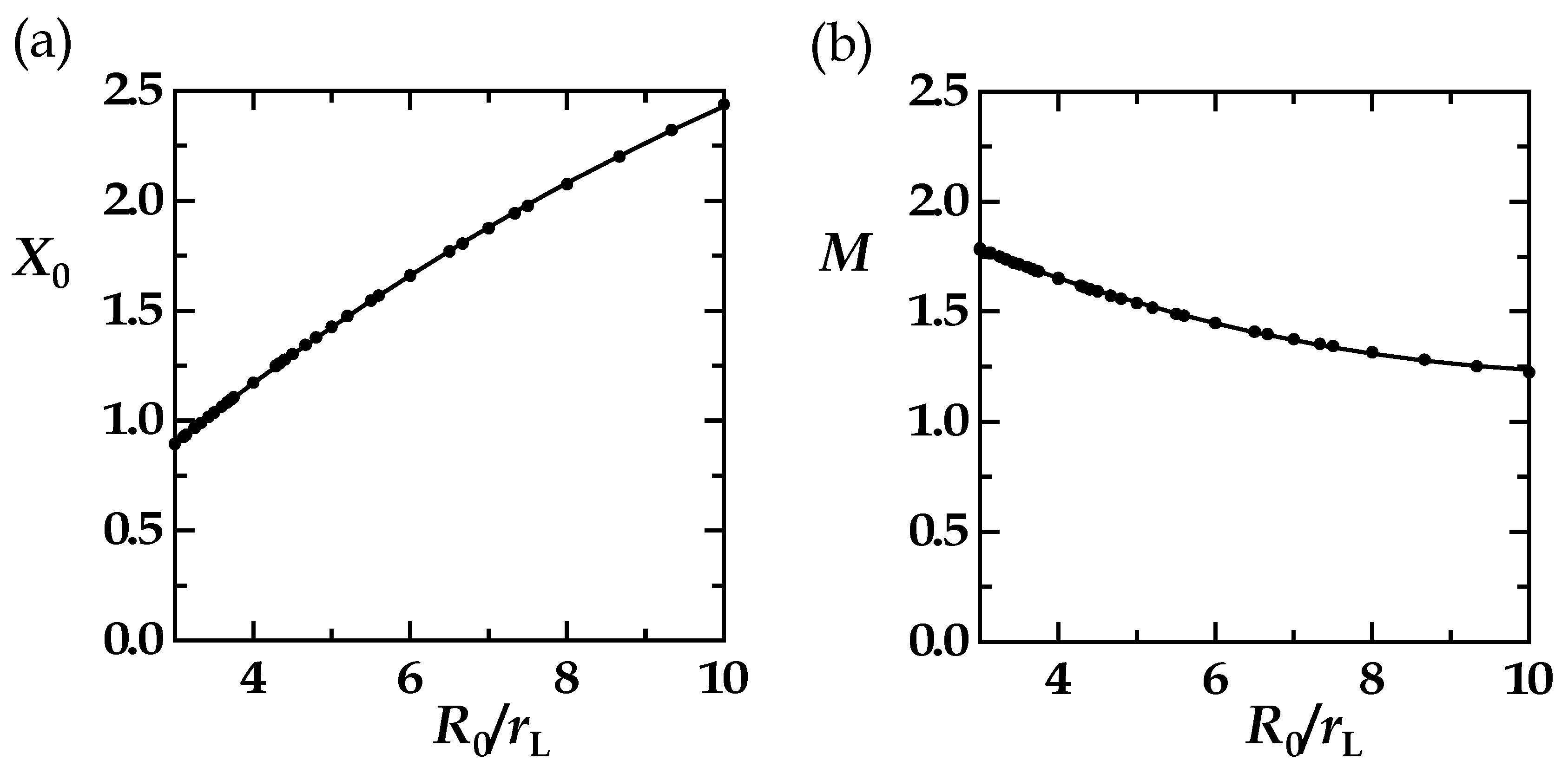
The figure illustrates how X0 and M vary with R0 for the two series when rL is kept at 3 Å. For M, the values obtained for the two series overlap (upper black and blue circles); for X0, the values (lower black and blue circles) obtained for the two series are so close that the corresponding diffusion profiles (see panel b) are visually indistinguishable.

3.4. The HSJE

We can now analyze the results obtained for X0 and M for the distribution series with b = 2R0, the series that guarantees highest numerical accuracy by leading to the largest ∆Reff = LR differences or DI(X) amplitudes. We obtained smooth curves that could be fitted to second-degree polynomial functions. Data points and fitting curves coincided (Figure 7). The functions and coefficients are given in Table 2.
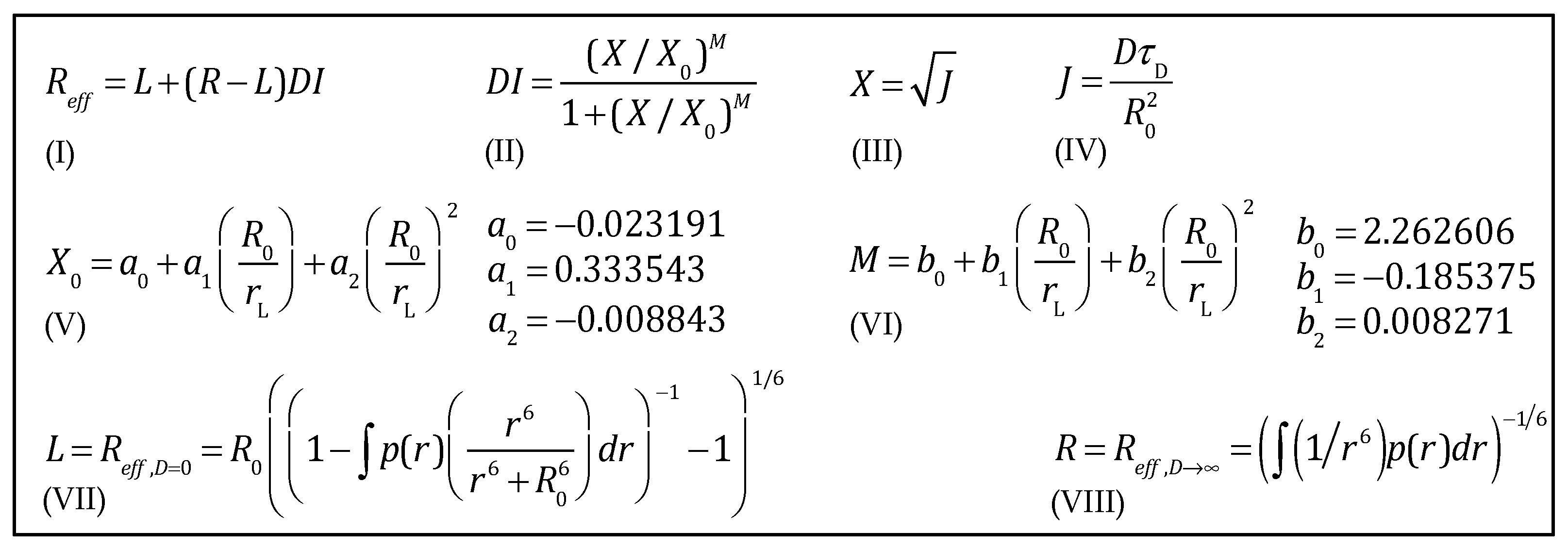
We are ready to state the HSJE for the given range of R0 = 9–15 Å and rL = 1.5–5 Å (see the legend of Figure 7) in Figure 8. For clarity, we have decomposed the HSJE into its simple constituents, equations (I) to (VIII). The HSJE written as a single equation is shown in Supporting Information, Chapter 7e.
We now have a closed analytical expression, a CAE, for a defined parameter range. As with any other equation, it can now be applied to global analyses. The preliminary insights gained from such applications are very interesting but not the main topic of this article. We therefore referred these first applications of the HSJE to the Supporting Information, Chapter 8, Figures S6a–d and S7a–d.

4. Discussion

We have followed the full path from a partial differential equation, the HSE, to a closed analytical expression, the HSJE. Its benefits are of a theoretical but also of a mere practical nature: The HSJE is usually solved in seconds, not in minutes or hours, by two orders of magnitude faster than the HSE. This advantage amplifies when the HSJE is used as the basis of a global analysis that generally requires numerous fitting cycles to reach the best values for the diffusion coefficient, D; the distance distribution, p(r); and the left-integration limit, rL. Experimental values of the effective distance can be obtained from time-resolved fluorescence measurements but equally well from more widely available steady-state fluorescence spectroscopy. The HSJE is certainly not trivial but is still simple enough that multivariate or global analysis can be performed in commonly available programs such as Microsoft Excel.
DFRET is just one method in a whole range of optical methods for studying the structure and dynamics of polymers [10,11,12,13,14,17,19,20,21,22,23,24,25,26,27,28,29,30,31,32,33,34,35,36,37,38,39,40,41,42,43,44,45,46,47,48,49,50,51,52,53,54,55,56,57,58,59,60,61,62]. When we go into detail, we realize that any progress in DFRET can synergistically promote progress in this entire field [13]. The structure and dynamics of polymers are so important that numerous methods based on two optical molecular labels have been developed [2,3,5,6,10,11,13,15,17,22,23,24,25,27,28,29,30,31,32,33,34,35,36,37,38,47,48,49,57,58,59,63,64,65,66,67,68]. These labels are either synthetically conjugated to the chain or naturally present, as, for instance, Trp or Tyr in a peptide or protein. One of the deepest motivations for developing such methods has always been the “protein folding problem”. The “static” folding problem now appears to have been solved by artificial intelligence methods applied to a huge amount of data [69] but countless questions about folding involving dynamics and mechanisms remain open. Examples include misfolding in amyloidosis diseases as well as the sometimes bizarre behavior of intrinsically disordered peptides and proteins [70].
These methods include not only FRET, but also CQ methods (collisional-quenching methods)1 [25,71]. For example, the sdFRET method is based on the excitation of a donor, e.g., the donor FTrp, in combination with Dbo as acceptor. The peculiarity of this FTrp/Dbo pair is that instead of FTrp, one can simply excite Dbo, whose fluorescence is then quenched by collision with FTrp [49]. This particular CQ method is called CIFQ (collision-induced fluorescence quenching). How quickly this quenching proceeds also informs the dynamics and flexibility of the chain. In the past, we have been able to reconcile seemingly contradictory results from different sdFRET, CIFQ, and CQ methods [13]. Therefore, we reiterate our assertion that any progress in DFRET or any of the other methods can synergistically promote progress in the entire field of polymer structure and dynamics. We believe that we have made such progress with the development of the HSJE.
The augmented diffusion coefficient. In addition to the practical benefits of the HSJE, we believe that its structure gives a more lucid insight into parameters whose variation can feed essential information into the needed global analysis. This is first of all the newly defined augmented diffusion coefficient, J. What does J actually mean? If we want to determine the diffusion impact and the diffusion coefficient, D, we need the widest possible range of the diffusion influence, DI, preferably from 0 to 100%. It is clear that any experimental series might cover a range within these limits but can never reach these limits themselves. We established that DI increases with J and that J increases linearly with D and τD, the donor lifetime, and decreases with the square root of the Förster radius, R0 (Equation (18)). All of these variations have been employed in earlier attempts at a global analysis but without knowing which range of the diffusion influence was actually covered [3,7,9,10,14]. In this work, we obtained certainty that our previous variation [14] of the diffusion coefficient by solvent viscosity and variation of the donor lifetime by adding the viscogen ethylene glycol and by going from the donor FTrp to the donor NAla covered a DI range of 8 to 80% (comp. Supporting Information, Chapter 8c). In previous works [12,14], we also investigated and discussed the role of the donor quantum yield, and we continue this discussion in Supporting Information, Chapter 9, because the donor quantum yield can be made part of the HSJE as shown in Equations (S31)–(S33).
Preview. In summary, the diffusion contribution to FRET should not be neglected whenever we are not close to the static limit. Therefore, the question remains up to which R0-values and under which circumstances are we not close to this limit. Up to which R0-values should diffusion be included into the analysis, and up to which values should the HSJE be extended?

5. Conclusions

Fluorescence methods and methods based on fluorescence resonance energy transfer have asserted their place in questions of molecular/bio-molecular structure and dynamics simply because their speed and sensitivity are unsurpassed. We believe that also diffusion-enhanced Förster resonance energy transfer or DFRET has the potential to become influential, although the number of publications based on it has been small to date. DFRET ensemble analysis has been based on a partial differential equation, on the HSE. Using the HSE in a global analysis means that profound challenges must first be overcome. Furthermore, even with seemingly successful fits, doubts often remain about the realistic significance of the results obtained. By replacing the PDE with a closed analytical expression, by replacing the HSE with the HSJE, these difficulties can be ended.

Supplementary Materials

The following supporting information can be downloaded at: https://www.mdpi.com/article/10.3390/polym15030705/s1, The document “Supporting information: Diffusion-Enhanced Förster Resonance Energy Transfer in Flexible Peptides: From the Haas-Steinberg Partial Differential Equation to a Closed Analytical Expression”, which provides a detailed glossary, a review of relevant previously published information, an overview of basic concepts, aids to understanding the new findings, an initial application of the HSJE in a global analysis, and an introduction to ongoing discussion points.

Author Contributions

Concepts and Analysis, M.H.J.; Funding acquisition, M.H.J. and W.M.N.; Numerical Simulations, M.H.J.; Software coding, R.N.D. and M.H.J.; Writing—original draft, M.H.J.; Discussions: A.I.L., W.M.N. and M.H.J.; Writing—review and editing, M.H.J. and W.M.N. All authors have read and agreed to the published version of the manuscript.

Funding

This research was funded by the German Research Foundation (DFG), grant number NA 686/9.

Institutional Review Board Statement

Not applicable.

Informed Consent Statement

Not applicable.

Data Availability Statement

Not applicable.

Acknowledgments

We thank the Deutsche Forschungsgemeinschaft (DFG, NA 686/9) for financial support. Special thanks to Jean Duhamel (University of Waterloo, Canada) for very valuable suggestions, to Sergiy Vasylkevych (University of Hamburg), and to Karenina Sender (University of Bremen) for critical review of the mathematics.

Conflicts of Interest

The authors declare no conflict of interest.

References

  1. Ingargiola, A.; Weiss, S.; Lerner, E. Monte Carlo Diffusion-Enhanced Photon Inference: Distance Distributions and Conformational Dynamics in Single-Molecule FRET. J. Phys. Chem. B 2018, 122, 11598–11615. [Google Scholar] [CrossRef] [PubMed] [Green Version]
  2. Förster, T. Zwischenmolekulare Energiewanderung und Fluoreszenz. Ann. Phys. 1948, 2, 55–75. [Google Scholar] [CrossRef]
  3. Haas, E.; Katchalski-Katzir, E.; Steinberg, I.Z. Brownian Motion of the Ends of Oligopeptides Chains in Solution as Estimated by Energy Transfer between the Chain Ends. Biopolymers 1978, 17, 11–31. [Google Scholar] [CrossRef]
  4. Stryer, L.; Thomas, D.D.; Meares, C.F. Diffusion-Enhanced Fluorescence Energy Transfer. Annu. Rev. Biophys. Bioeng. 1982, 11, 203–222. [Google Scholar] [CrossRef] [PubMed]
  5. Beechem, J.M.; Haas, E. Simultaneous Determination of Intramolecular Distance Distributions and Conformational Dynamics by Global Analysis of Energy Transfer Measurements. Biophys. J. 1989, 55, 1225–1236. [Google Scholar] [CrossRef] [Green Version]
  6. Lakowicz, J.R.; Kusba, J.; Gryczynski, I.; Wiczk, W.; Szmacinski, H.; Johnson, M.L. End-to-End Diffusion and Distance Distributions of Flexible Donor-Acceptor Systems Observed by Intramolecular Energy-Transfer and Frequency-Domain Fluorometry—Enhanced Resolution by Global Analysis of Externally Quenched and Nonquenched Samples. J. Phys. Chem. B 1991, 95, 9654–9660. [Google Scholar] [CrossRef]
  7. Maliwal, B.P.; Kusba, J.; Wiczk, W.; Johnson, M.L.; Lakowicz, J.R. End-to-End Diffusion Coefficients and Distance Distributions from Fluorescence Energy Transfer Measurements: Enhanced Resolution by Using Multiple Acceptors with Different Förster Distances. Biophys. Chem. 1993, 46, 273–281. [Google Scholar] [CrossRef]
  8. Steinberg, I.Z. Brownian Motion of the End-to-End Distance in Oligopeptide Molecules: Numerical Solution of the Diffusion Equations as Coupled First Order Linear Differential Equations. J. Theor. Biol. 1994, 166, 173–187. [Google Scholar] [CrossRef] [PubMed]
  9. Gryczynski, I.; Lakowicz, J.R.; Kusba, J. End-to-End Diffusion Coefficients and Distance Distributions from Fluorescence Energy Transfer Measurements: Enhanced Resolution by Using Multiple Donors with Different Lifetimes. J. Fluoresc 1995, 5, 195–203. [Google Scholar] [CrossRef]
  10. Möglich, A.; Joder, K.; Kiefhaber, T. End-to-End Distance Distributions and Intrachain Diffusion Constants in Unfolded Polypeptide Chains Indicate Intramolecular Hydrogen Bond Formation. Proc. Natl. Acad. Sci. USA 2006, 103, 12394–12399. [Google Scholar] [CrossRef] [Green Version]
  11. Grupi, A.; Haas, E. Segmental Conformational Disorder and Dynamics in the Intrinsically Disordered Protein Alpha-Synuclein and Its Chain Length Dependence. J. Mol. Biol. 2011, 405, 1267–1283. [Google Scholar] [CrossRef]
  12. Jacob, M.H.; Dsouza, R.N.; Ghosh, I.; Norouzy, A.; Schwarzlose, T.; Nau, W.M. Diffusion-Enhanced Forster Resonance Energy Transfer and the Effects of External Quenchers and the Donor Quantum Yield. J. Phys. Chem. B 2013, 117, 185–198. [Google Scholar] [CrossRef] [PubMed]
  13. Jacob, M.H.; D’Souza, R.N.; Schwarzlose, T.; Wang, X.; Huang, F.; Haas, E.; Nau, W.M. Method-Unifying View of Loop-Formation Kinetics in Peptide and Protein Folding. J. Phys. Chem. B 2018, 122, 4445–4456. [Google Scholar] [CrossRef] [PubMed]
  14. Jacob, M.H.; Ghosh, I.; D’Souza, R.N.; Nau, W.M. Two Orders of Magnitude Variation of Diffusion-Enhanced Förster Resonance Energy Transfer in Polypeptide Chains. Polymers 2018, 10, 1079. [Google Scholar] [CrossRef] [Green Version]
  15. Lerner, E.; Orevi, T.; Ben Ishay, E.; Amir, D.; Haas, E. Kinetics of Fast Changing Intramolecular Distance Distributions Obtained by Combined Analysis of Fret Efficiency Kinetics and Time-Resolved Fret Equilibrium Measurements. Biophys. J. 2014, 106, 667–676. [Google Scholar] [CrossRef] [PubMed] [Green Version]
  16. May, V.; Kühn, O. Charge and Energy Transfer Dynamics in Molecular Systems; Wiley-VCH: Berlin, Germany, 2000. [Google Scholar]
  17. Sahoo, H.; Roccatano, D.; Zacharias, M.; Nau, W.M. Distance Distributions of Short Polypeptides Recovered by Fluorescence Resonance Energy Transfer in the 10 Å Domain. J. Am. Chem. Soc. 2006, 128, 8118–8119. [Google Scholar] [CrossRef]
  18. Jacob, M.H.; Nau, W.M. Short-Distance FRET Applied to the Polypeptide Chain. In Folding, Misfolding and Nonfolding of Peptides and Small Proteins; Schweitzer-Stenner, R., Ed.; John Wiley & Sons: Hoboken, NJ, USA, 2011. [Google Scholar]
  19. Casier, R.; Duhamel, J. Pyrene Excimer Fluorescence as a Direct and Easy Experimental Means to Characterize the Length Scale and Internal Dynamics of Polypeptide Foldons. Macromolecules 2018, 51, 3450–3457. [Google Scholar] [CrossRef]
  20. Orevi, T.; Lerner, E.; Rahamim, G.; Amir, D.; Haas, E. Ensemble and Single-Molecule Detected Time-Resolved Fret Methods in Studies of Protein Conformations and Dynamics. Methods. Mol. Biol. 2014, 1076, 113–169. [Google Scholar]
  21. Stryer, L. Fluorescence Energy Transfer as a Spectroscopic Ruler. Ann. Rev. Biochem. 1978, 47, 819–846. [Google Scholar] [CrossRef]
  22. Duhamel, J.; Yekta, A.; Winnik, M.A.; Jao, T.C.; Mishra, M.K.; Rubin, I.D. A Blob Model to Study Polymer Chain Dynamics in Solution. J. Phys. Chem. 1993, 97, 13708–13712. [Google Scholar] [CrossRef]
  23. Weiss, S. Measuring Conformational Dynamics of Biomolecules by Single Molecule Fluorescence Spectroscopy. Nat. Struct. Biol. 2000, 7, 724–729. [Google Scholar] [CrossRef] [PubMed]
  24. Broos, J.; Pas, H.H.; Robillard, G.T. The Smallest Resonance Energy Transfer Acceptor for Tryptophan. J. Am. Chem. Soc. 2002, 124, 6812–6813. [Google Scholar] [CrossRef] [Green Version]
  25. Hudgins, R.R.; Huang, F.; Gramlich, G.; Nau, W.M. A Fluorescence-Based Method for Direct Measurement of Submicrosecond Intramolecular Contact Formation in Biopolymers: An Exploratory Study with Polypeptides. J. Am. Chem. Soc. 2002, 124, 556–564. [Google Scholar] [CrossRef]
  26. Duhamel, J.; Kanagalingam, S.; O’Brien, T.J.; Ingratta, M.W. Side-Chain Dynamics of an Alpha-Helical Polypeptide Monitored by Fluorescence. J. Am. Chem. Soc. 2003, 125, 12810–12822. [Google Scholar] [CrossRef] [PubMed]
  27. Nau, W.M.; Huang, F.; Wang, X.J.; Bakirci, H.; Gramlich, G.; Marquez, C. Exploiting Long-Lived Molecular Fluorescence. Chimia 2003, 57, 161–167. [Google Scholar] [CrossRef]
  28. Schuler, B.; Lipman, E.A.; Steinbach, P.J.; Kumke, M.; Eaton, W.A. Polyproline and the “Spectroscopic Ruler” Revisited with Single- Molecule Fluorescence. Proc. Natl. Acad. Sci. USA 2005, 102, 2754–2759. [Google Scholar] [CrossRef] [PubMed] [Green Version]
  29. Duhamel, J. Polymer Chain Dynamics in Solution Probed with a Fluorescence Blob Model. Acc. Chem. Res. 2006, 39, 953–960. [Google Scholar] [CrossRef] [PubMed]
  30. Sahoo, H.; Nau, W.M. Phosphorylation-Induced Conformational Changes in Short Peptides Probed by Fluorescence Resonance Energy Transfer in the 10-Å Domain. ChemBioChem 2007, 8, 567–573. [Google Scholar] [CrossRef]
  31. Sahoo, H.; Roccatano, D.; Hennig, A.; Nau, W.M. A 10-a Spectroscopic Ruler Applied to Short Polyprolines. J. Am. Chem. Soc. 2007, 129, 9762–9772. [Google Scholar] [CrossRef]
  32. Schuler, B. Application of Single Molecule Forster Resonance Energy Transfer to Protein Folding. Methods Mol. Biol. 2007, 350, 115–138. [Google Scholar]
  33. Glasscock, J.M.; Zhu, Y.J.; Chowdhury, P.; Tang, J.; Gai, F. Using an Amino Acid Fluorescence Resonance Energy Transfer Pair to Probe Protein Unfolding: Application to the Villin Headpiece Subdomain and the Lysm Domain. Biochemistry 2008, 47, 11070–11076. [Google Scholar] [CrossRef] [PubMed] [Green Version]
  34. Haas, E. Protein Folding Handbook; Buchner, K., Ed.; John Wiley & Sons: Hoboken, NJ, USA, 2008. [Google Scholar]
  35. Ingratta, M.; Duhamel, J. Effect of Side-Chain Length on the Side-Chain Dynamics of Alpha-Helical Poly(L-Glutamic Acid) as Probed by a Fluorescence Blob Model. J. Phys. Chem. B 2008, 112, 9209–9218. [Google Scholar] [CrossRef] [PubMed]
  36. Ingratta, M.; Hollinger, J.; Duhamel, J. A Case for Using Randomly Labeled Polymers to Study Long-Range Polymer Chain Dynamics by Fluorescence. J. Am. Chem. Soc. 2008, 130, 9420–9428. [Google Scholar] [CrossRef] [PubMed]
  37. Khan, Y.R.; Dykstra, T.E.; Scholes, G.D. Exploring the Förster Limit in a Small FRET Pair. Chem. Phys. Lett. 2008, 461, 305–309. [Google Scholar] [CrossRef]
  38. Orevi, T.; Ishay, E.B.; Pirchi, M.; Jacob, M.H.; Amir, D.; Haas, E. Early Closure of a Long Loop in the Refolding of Adenylate Kinase: A Possible Key Role of Non-Local Interactions in the Initial Folding Steps. J. Mol. Biol. 2009, 385, 1230–1242. [Google Scholar] [CrossRef]
  39. Chen, S.; Duhamel, J.; Winnik, M.A. Probing End-to-End Cyclization Beyond Willemski and Fixman. J. Phys. Chem. B 2011, 115, 3289–3302. [Google Scholar] [CrossRef]
  40. Grupi, A.; Haas, E. Time-Resolved Fret Detection of Subtle Temperature-Induced Conformational Biases in Ensembles of Alpha-Synuclein Molecules. J. Mol. Biol. 2011, 411, 234–247. [Google Scholar] [CrossRef]
  41. Ben Ishay, E.; Rahamim, G.; Orevi, T.; Hazan, G.; Amir, D.; Haas, E. Fast Subdomain Folding Prior to the Global Refolding Transition of E. coli Adenylate Kinase: A Double Kinetics Study. J. Mol. Biol. 2012, 423, 613–623. [Google Scholar] [CrossRef]
  42. Fowler, M.A.; Duhamel, J.; Bahun, G.J.; Adronov, A.; Zaragoza-Galan, G.; Rivera, E. Studying Pyrene-Labeled Macromolecules with the Model-Free Analysis. J. Phys. Chem. B 2012, 116, 14689–14699. [Google Scholar] [CrossRef]
  43. Chen, S.; Duhamel, J. Probing the Hydrophobic Interactions of a Series of Pyrene End-Labeled Poly(Ethylene Oxide)S in Aqueous Solution Using Time-Resolved Fluorescence. Langmuir 2013, 29, 2821–2834. [Google Scholar] [CrossRef]
  44. Lerner, E.; Hilzenrat, G.; Amir, D.; Tauber, E.; Garini, Y.; Haas, E. Preparation of Homogeneous Samples of Double-Labelled Protein Suitable for Single-Molecule Fret Measurements. Anal. Bioanal. Chem. 2013, 405, 5983–5991. [Google Scholar] [CrossRef] [PubMed]
  45. Orevi, T.; Rahamim, G.; Hazan, G.; Amir, D.; Haas, E. The Loop Hypothesis: Contribution of Early Formed Specific Non-Local Interactions to the Determination of Protein Folding Pathways. Biophys. Rev. 2013, 5, 85–98. [Google Scholar] [CrossRef] [PubMed] [Green Version]
  46. Duhamel, J. Global Analysis of Fluorescence Decays to Probe the Internal Dynamics of Fluorescently Labeled Macromolecules. Langmuir 2014, 30, 2307–2324. [Google Scholar] [CrossRef] [PubMed]
  47. Orevi, T.; Ben Ishay, E.; Gershanov, S.L.; Dalak, M.B.; Amir, D.; Haas, E. Fast Closure of N-Terminal Long Loops but Slow Formation of Beta Strands Precedes the Folding Transition State of Escherichia coli Adenylate Kinase. Biochemistry 2014, 53, 3169–3178. [Google Scholar] [CrossRef]
  48. Zaragoza-Galán, G.; Fowler, M.; Rein, R.; Solladié, N.; Duhamel, J.; Rivera, E. Fluorescence Resonance Energy Transfer in Partially and Fully Labeled Pyrene Dendronized Porphyrins Studied with Model Free Analysis. J. Phys. Chem. C 2014, 118, 8280–8294. [Google Scholar] [CrossRef]
  49. Norouzy, A.; Assaf, K.I.; Zhang, S.; Jacob, M.H.; Nau, W.M. Coulomb Repulsion in Short Polypeptides. J. Phys. Chem. B 2015, 119, 33–43. [Google Scholar] [CrossRef]
  50. Rahamim, G.; Chemerovski-Glikman, M.; Rahimipour, S.; Amir, D.; Haas, E. Resolution of Two Sub-Populations of Conformers and Their Individual Dynamics by Time Resolved Ensemble Level Fret Measurements. PLoS ONE 2015, 10, e0143732. [Google Scholar] [CrossRef] [PubMed] [Green Version]
  51. Toptygin, D. Effect of Diffusion on Resonance Energy Transfer Rate Distributions: Implications for Distance Measurements. J. Phys. Chem. B 2015, 119, 12603–12622. [Google Scholar] [CrossRef]
  52. Duhamel, J. Long Range Polymer Chain Dynamics Studied by Fluorescence Quenching. Macromolecules 2016, 49, 6149–6162. [Google Scholar]
  53. Orevi, T.; Rahamim, G.; Amir, D.; Kathuria, S.; Bilsel, O.; Matthews, C.R.; Haas, E. Sequential Closure of Loop Structures Forms the Folding Nucleus During the Refolding Transition of the Escherichia coli Adenylate Kinase Molecule. Biochemistry 2016, 55, 79–91. [Google Scholar] [CrossRef]
  54. Peulen, T.O.; Opanasyuk, O.; Seidel, C.A.M. Combining Graphical and Analytical Methods with Molecular Simulations to Analyze Time-Resolved FRET Measurements of Labeled Macromolecules Accurately. J. Phys. Chem. B 2017, 121, 8211–8241. [Google Scholar] [CrossRef] [PubMed] [Green Version]
  55. Song, J.; Gomes, G.N.; Shi, T.; Gradinaru, C.C.; Chan, H.S. Conformational Heterogeneity and Fret Data Interpretation for Dimensions of Unfolded Proteins. Biophys. J. 2017, 113, 1012–1024. [Google Scholar] [CrossRef] [PubMed] [Green Version]
  56. Wallace, B.; Atzberger, P.J. Forster Resonance Energy Transfer: Role of Diffusion of Fluorophore Orientation and Separation in Observed Shifts of Fret Efficiency. PLoS ONE 2017, 12, e0177122. [Google Scholar] [CrossRef] [PubMed] [Green Version]
  57. Eilert, T.; Kallis, E.; Nagy, J.; Röcker, C.; Michaelis, J. Complete Kinetic Theory of Fret. J. Phys. Chem. B 2018, 122, 1677–11694. [Google Scholar] [CrossRef]
  58. Qin, L.; Li, L.; Sha, Y.; Wang, Z.; Zhou, D.; Chen, W.; Xue, G. Conformational Transitions of Polymer Chains in Solutions Characterized by Fluorescence Resonance Energy Transfer. Polymers 2018, 10, 1007. [Google Scholar] [CrossRef] [Green Version]
  59. Ahmed, I.A.; Rodgers, J.M.; Eng, C.; Troxler, T.; Gai, F. Pet and Fret Utility of an Amino Acid Pair: Tryptophan and 4-Cyanotryptophan. Phys. Chem. Chem. Phys. 2019, 21, 12843–12849. [Google Scholar] [CrossRef]
  60. Duhamel, J. The Effect of Amino Acid Size on the Internal Dynamics and Conformational Freedom of Polypeptides. Macromolecules 2020, 53, 9811–9822. [Google Scholar]
  61. Duhamel, J. Characterization of the Local Volume Probed by the Side-Chain Ends of Poly(Oligo(Ethylene Glycol) 1-Pyrenemethyl Ether Methacrylate) Bottle Brushes in Solution Using Pyrene Excimer Fluorescence. Macromolecules 2021, 54, 9341–9350. [Google Scholar]
  62. Norouzy, A.; Lazar, A.I.; Karimi-Jafari, M.H.; Firouzi, R.; Nau, W.M. Electrostatically Induced Pk a Shifts in Oligopeptides: The Upshot of Neighboring Side Chains. Amino Acids 2022, 54, 277–287. [Google Scholar] [CrossRef]
  63. Stryer, L.; Haugland, R.P. Energy Transfer: A Spectroscopic Ruler. Proc. Natl. Acad. Sci. USA 1967, 58, 719–726. [Google Scholar] [CrossRef] [Green Version]
  64. Ha, T. Single-Molecule Fluorescence Resonance Energy Transfer. Methods 2001, 25, 78–86. [Google Scholar] [CrossRef] [Green Version]
  65. Haas, E. The Study of Protein Folding and Dynamics by Determination of Intramolecular Distance Distributions and Their Fluctuations Using Ensemble and Single-Molecule Fret Measurements. ChemPhysChem 2005, 6, 858–870. [Google Scholar] [CrossRef]
  66. Jacob, M.H.; Amir, D.; Ratner, V.; Gussakowsky, E.; Haas, E. Predicting Reactivities of Protein Surface Cysteines as Part of a Strategy for Selective Multiple Labeling. Biochemistry 2005, 44, 13664–13672. [Google Scholar] [CrossRef] [PubMed]
  67. Siu, H.; Duhamel, J. Comparison of the Association Level of a Pyrene-Labeled Associative Polymer Obtained from an Analysis Based on Two Different Models. J. Phys. Chem. B 2005, 109, 1770–1780. [Google Scholar] [CrossRef] [PubMed]
  68. Gopich, I.V.; Szabo, A. Single-Molecule FRET with Diffusion and Conformational Dynamics. J. Phys. Chem. B 2007, 111, 12925–12932. [Google Scholar] [CrossRef] [PubMed]
  69. Jumper, J.; Evans, R.; Pritzel, A.; Green, T.; Figurnov, M.; Ronneberger, O.; Tunyasuvunakool, K.; Bates, R.; Žídek, A.; Potapenko, A.; et al. Highly Accurate Protein Structure Prediction with Alphafold. Nature 2021, 596, 583–589. [Google Scholar] [CrossRef]
  70. Pinheiro, F.; Santos, J.; Ventura, S. Alphafold and the Amyloid Landscape. J. Mol. Biol. 2021, 433, 167059. [Google Scholar] [CrossRef]
  71. Bieri, O.; Wirz, J.; Hellrung, B.; Schutkowski, M.; Drewello, M.; Kiefhaber, T. The Speed Limit for Protein Folding Measured by Triplet-Triplet Energy Transfer. Proc. Natl. Acad. Sci. USA 1999, 96, 9597–9601. [Google Scholar] [CrossRef] [Green Version]
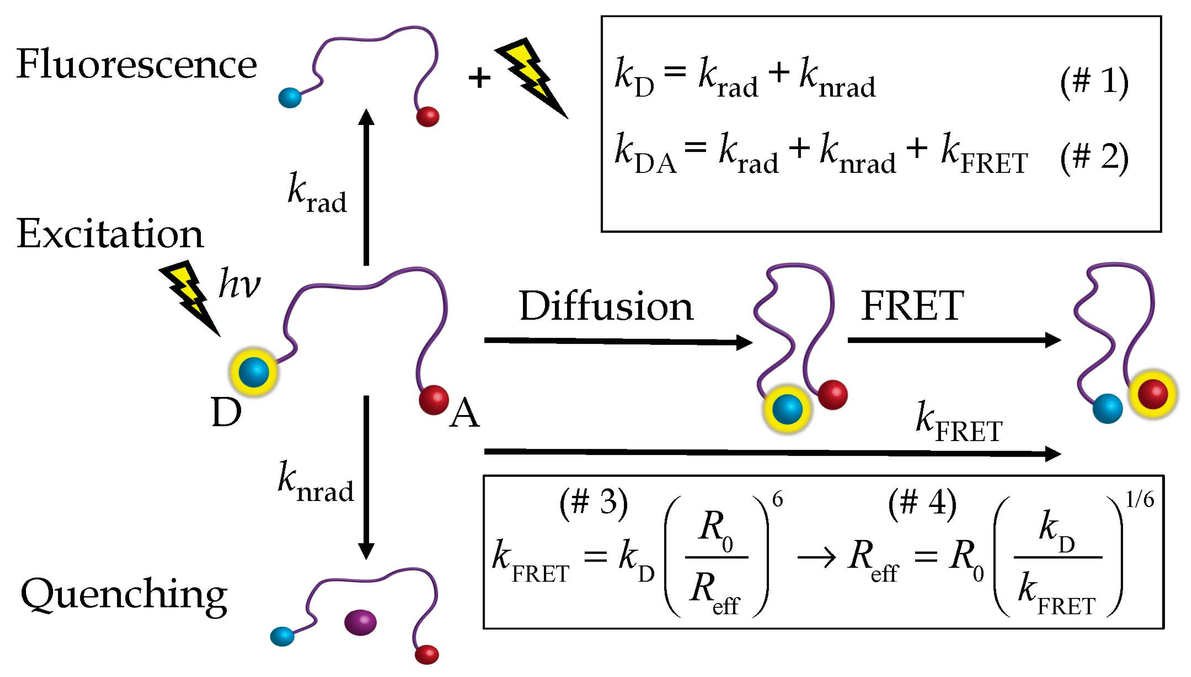
Figure 1. DFRET: Diffusion-enhanced Förster resonance energy transfer. After excitation, the excited donor, D, can either become deactivated by emitting fluorescence (krad) or by being quenched, for instance, by iodine ions (knrad) or by transferring its excitation energy to the acceptor, A (kFRET). FRET can take place at every D-A distance but is more likely to happen at shorter distances, which is why it is enhanced by D-A diffusion. The pertinent equations (I–IV) are explained in the main text.
Polymers 15 00705 g001
Figure 2. (a) An exemplary probability distance distribution of the donor–acceptor distance in a linear (bio)polymer (b) The diffusion profile or Reff (D1/2) profile: Solving the HSE under variation of the diffusion coefficient results in values of the effective distance that range from L to R (dashed lines). The effective distance plotted against D1/2 approaches Reff = L when the extent of diffusional motion approaches zero and approaches Reff = R when the extent of diffusional motion approaches infinity. (c) The diffusion-influence profile or DI(D1/2) profile is obtained when the diffusion profile shown in (b) is normalized with L and R according to DI = (ReffL)/(RL) (Equation (11)). The diffusion influence, DI, can adapt values between 0 (0%) and 1 (100%). (d) The diffusion-influence profile, the DI(J1/2) or DI(X) profile: The diffusion influence plotted against the square root of the augmented diffusion coefficient, X = J1/2 (see Equation (12)).
Polymers 15 00705 g002
Figure 3. (a) Three different 3-D Gaussian distance distributions (black, red, blue). (b) The corresponding diffusion profiles (black, red, blue) with the effective distance plotted against the square root of the diffusion coefficient. The donor lifetime, the Förster radius, and the left integration limit were kept constant (τD = 100 ns, R0 = 10 Å, rL = 2.5 Å) (c) After normalization (Equation (11)), the three profiles became identical.
Polymers 15 00705 g003
Figure 4. (a) A 3-D Gaussian distance distribution (b) Four diffusion profiles obtained with (a) four different donor lifetime constants, τD, of 100 ns (red), of 30 ns (blue), of 10 ns (green), and of 1 ns (black). The Förster radius (R0 = 15 Å) and the left integration limit (rL = 3 Å) were held constant. (c) Diffusion-influence profiles after normalization. (d) The DI-profiles coincide when the DI values are plotted against the square root of the product of diffusion coefficient and donor lifetime.
Polymers 15 00705 g004
Figure 5. (a) Three ideal-chain distance distributions (Equation (18)) with b = 18 Å, rL = 3 Å (black curve); b = 24 Å, rL = 4 Å (red curve); and b = 30 Å, rL = 5 Å (blue curve). (b) The corresponding diffusion profiles obtained with b = 18 Å, rL = 3 Å, R0 = 9 Å (black curve); with b = 24 Å, rL = 4 Å, R0 = 12 Å (red curve); and with b = 30 Å, rL = 5 Å, R0 = 15 Å (blue curve). Thus, for all three evaluated distributions (black, red, blue), the ratio R0/rL equaled 3. (c) The corresponding diffusion-influence profiles with DI plotted against X (X = J1/2). The three profiles merge into one.
Polymers 15 00705 g005
Figure 6. The HSE was solved for two different series of ideal-chain distributions (Equation (18)). R0 was varied from 9 Å to 15 Å, and rL was varied from 1.5 Å to 5 Å. The donor lifetime was held constant (τD = 100 ns). In one series of distributions, the constant b was chosen as b = 1.5⋅R0 ranging from 13.5 Å to 22.5 Å, in the other series as b = 2⋅R0 ranging from 18 Å to 30 Å. (a) Exemplary distributions for the two series with rL = 3 Å, R0 = 10 Å and either b = 1.5⋅R0 = 15 Å (blue curve) or b = 2⋅R0 = 20 Å (black curve). (b) The DI(X) profiles overlap for both distributions shown in (a). (c) All DI(X) profiles were analyzed by using Equation (13).
Polymers 15 00705 g006
Figure 7. The results for X0 and M (solid circles in panels (a,b) obtained for the range of R0 = 9–15 Å, rL = 1.5–5 Å with b = 2R0, and R0/rL > 3) were fitted to second-degree polynomial functions (solid lines in panels (a,b) given in Table 2).
Polymers 15 00705 g007
Figure 8. The Haas-Steinberg–Jacob equation (HSJE) is a closed analytical equation decomposed here into simple equations, I to VIII, for clarity. With the coefficients shown here (a0 to b3), it is valid for R0 9–15 Å and rL 1.5–5 Å.
Polymers 15 00705 g008
Table 1. Fitting results for X0 and M *.
R0/rLR0rLX0M
3930.89351.7823
31240.89291.7876
31550.89331.7861
4102.51.17221.6513
41231.17191.6532
4143.51.17241.6494
51021.42591.5387
51531.42561.5391
691.51.65911.4481
61221.65921.4483
6152.51.65871.4483
* The test distributions were chosen to follow Equation (18) with b = 2R0.
Table 2. X0 and M as second-degree polynomial functions of R0/rL.
X0 = a0 + a1 × (R0/rL) + a2 × (R0/rL)2; M = b0 + b1 × (R0/rL) + b2 × (R0/rL)2
nX0 =an-valueM =bn-value
0a0−0.023191b02.262606
1a1 × (R0/rL)0.333543b1 × (R0/rL)−0.185375
2a2 × (R0/rL)2−0.008843b2 × (R0/rL)20.008271
The coefficients a0, a1, a2, and b0, b1, b2 are valid for the conditions R0 = 9–15 Å, rL = 1.5–5 Å, R0/rL > 3.
Disclaimer/Publisher’s Note: The statements, opinions and data contained in all publications are solely those of the individual author(s) and contributor(s) and not of MDPI and/or the editor(s). MDPI and/or the editor(s) disclaim responsibility for any injury to people or property resulting from any ideas, methods, instructions or products referred to in the content.