
Analysis of the Machine-Specific Behavior of Injection Molding Machines


Abstract
:1. Introduction
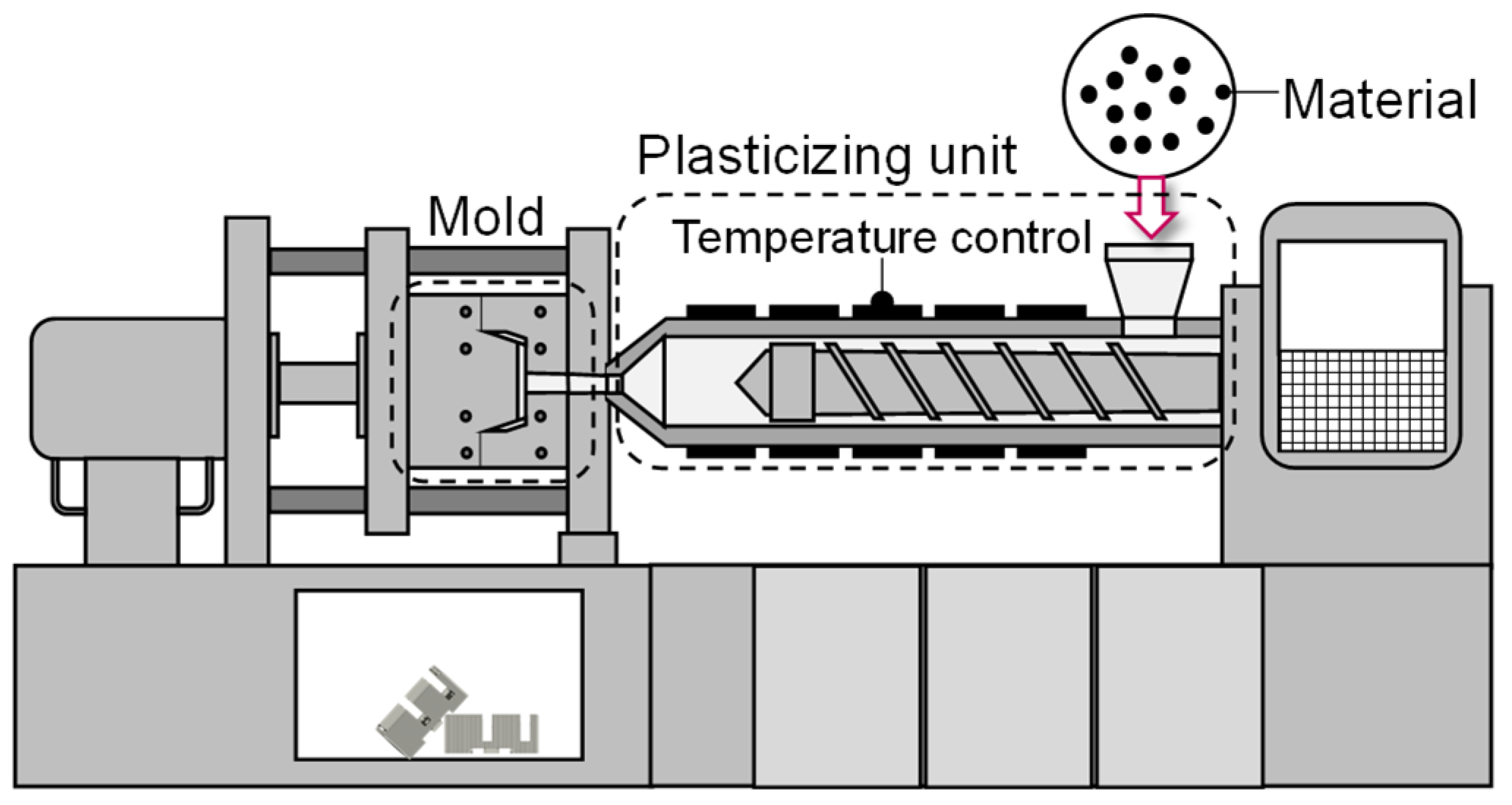
Influence of the Machine during the Injection Molding Process
- How does the machine-specific behavior of the machine influence the process when it is started from a cold state?
- How much do the processes differ when using different machines? What influence do the operating points have in each case?
- Do changes in the material characteristics affect the machine-specific behavior?
2. Materials and Methods
3. Results and Discussion
3.1. Part A: Evaluation of the Start-Up Behavior Based on the Ejected Polymer Masses
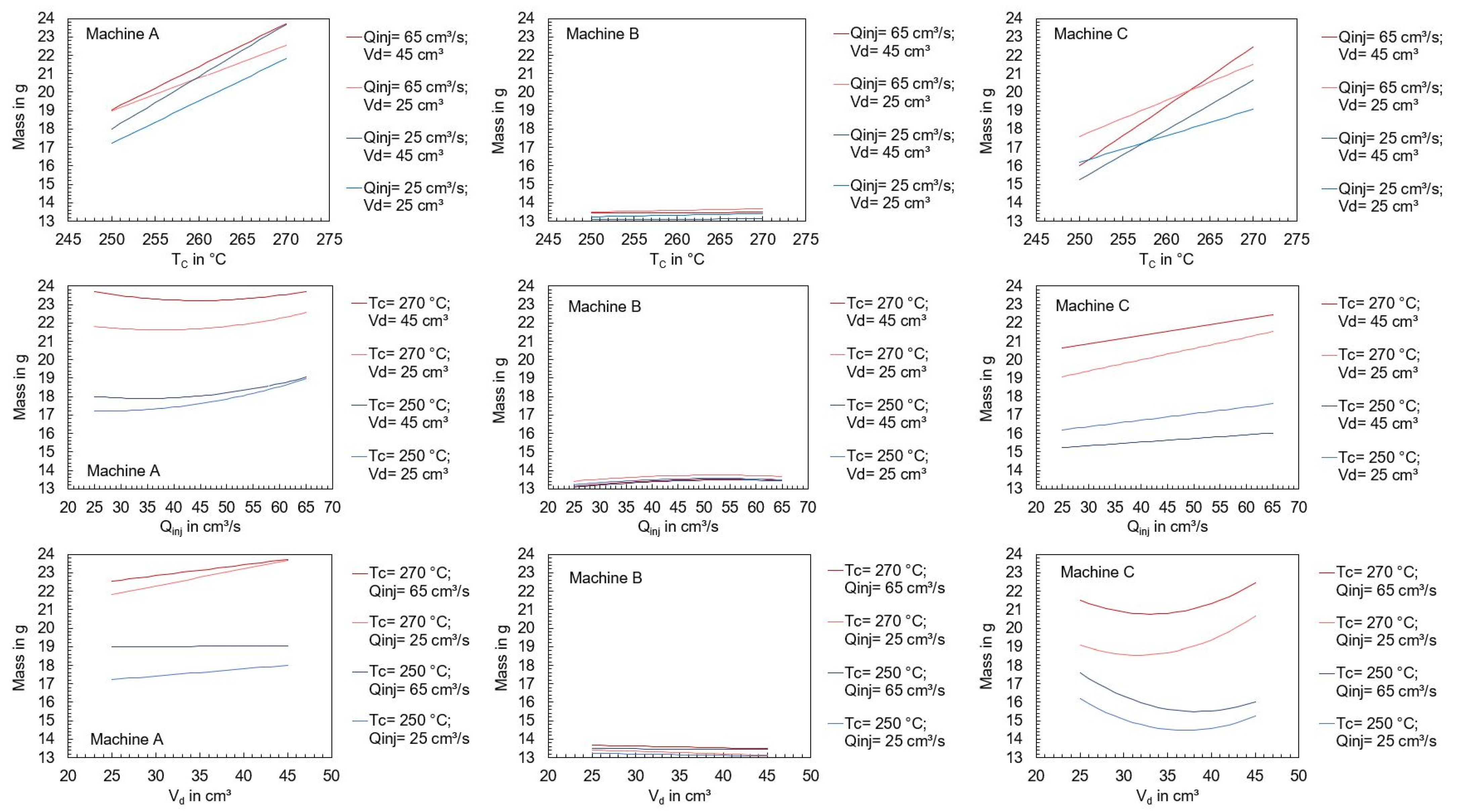
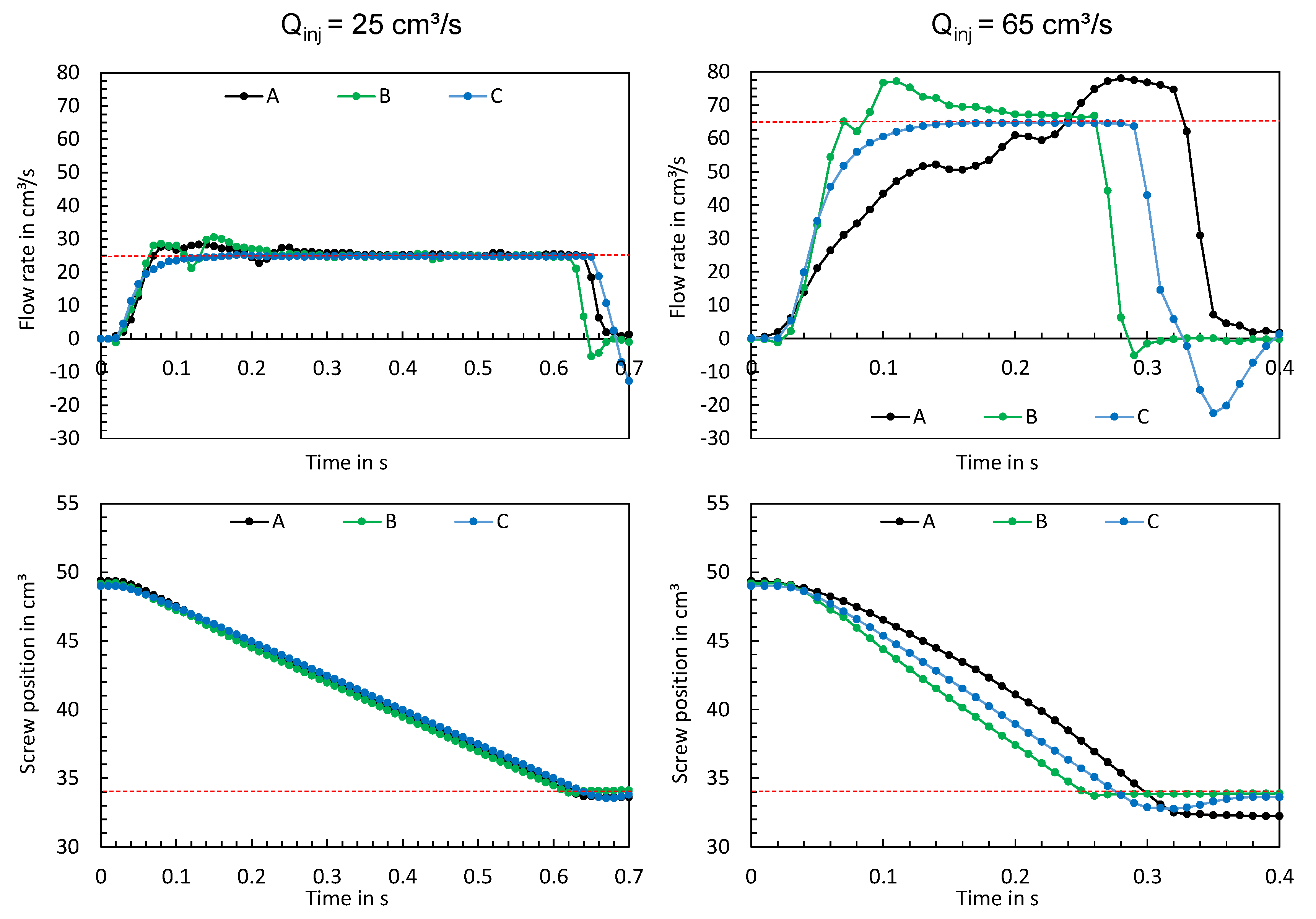
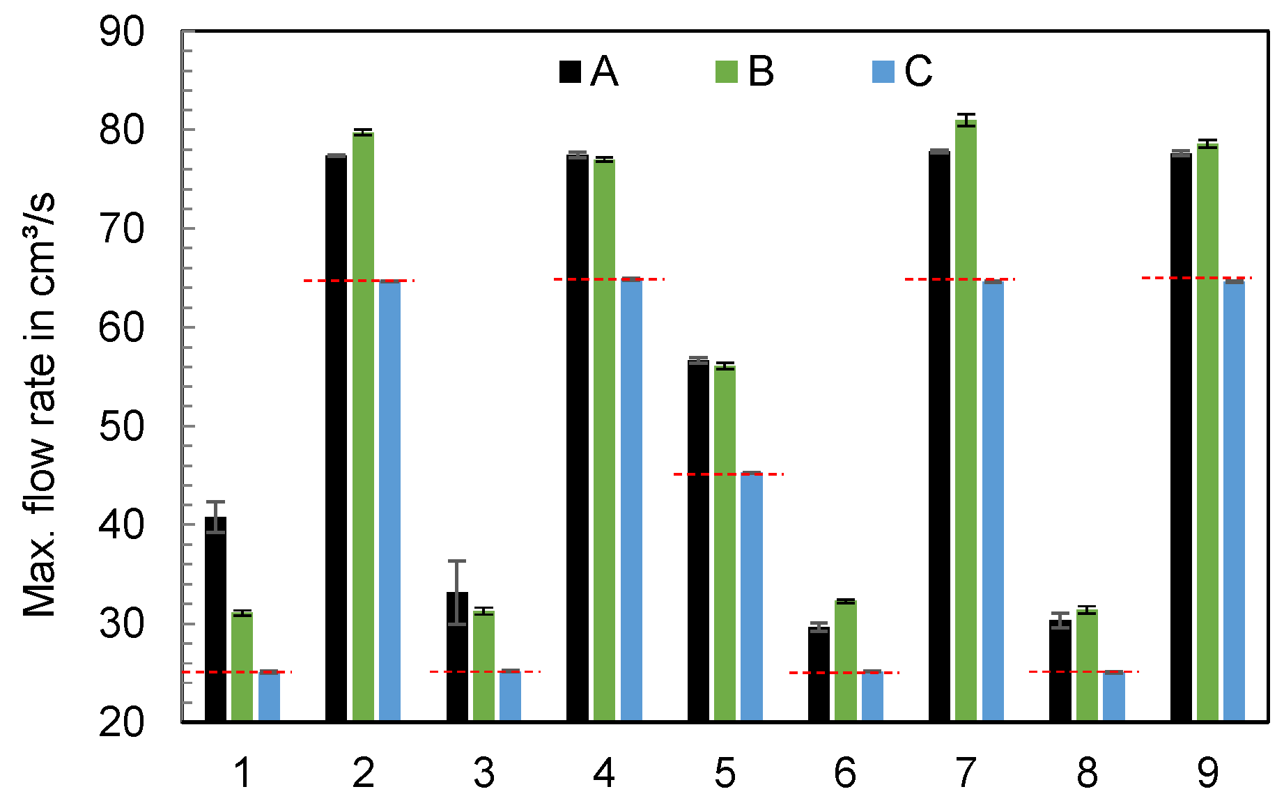
3.2. Part B: Analysis of the Machine-Specific Behavior of Three Different IMMs at Varying Operating Points
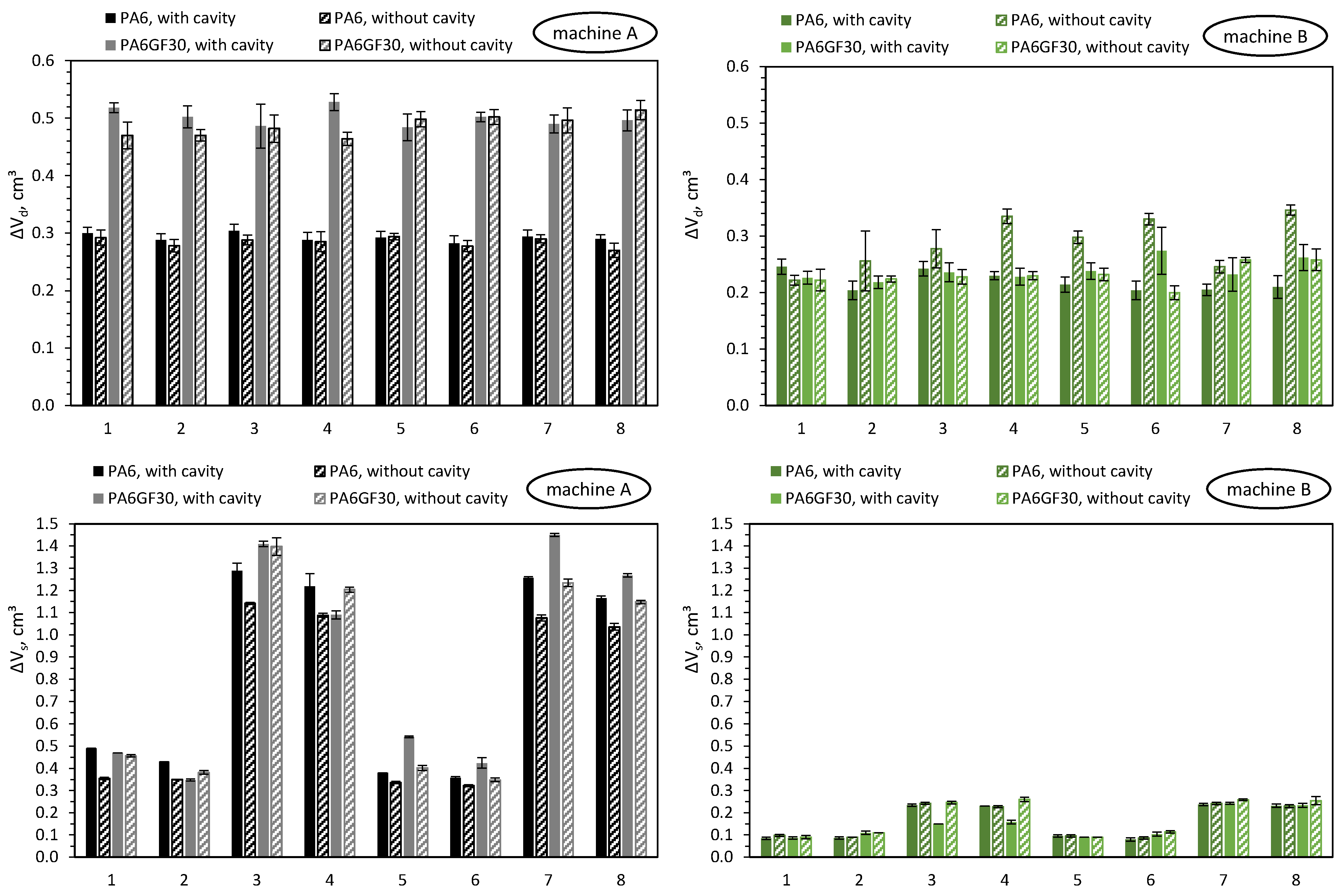
3.3. Part C: Influence of the Material on the Machine-Specific Behavior of Two Different Hydraulic Injection Molding Machines
4. Conclusions
- During the initial machine start-up phase, distinct variations in machine behavior were observed. These variations were assessed by analyzing the ejected polymer mass from shot to shot. The primary insight gained from this investigation is that the machine has a significant influence on the start-up behavior and the duration until a reproducible process characterized by mass stability is achieved. Sampling at the beginning of an experiment can thus be superposed by machine-specific thermal transient processes.
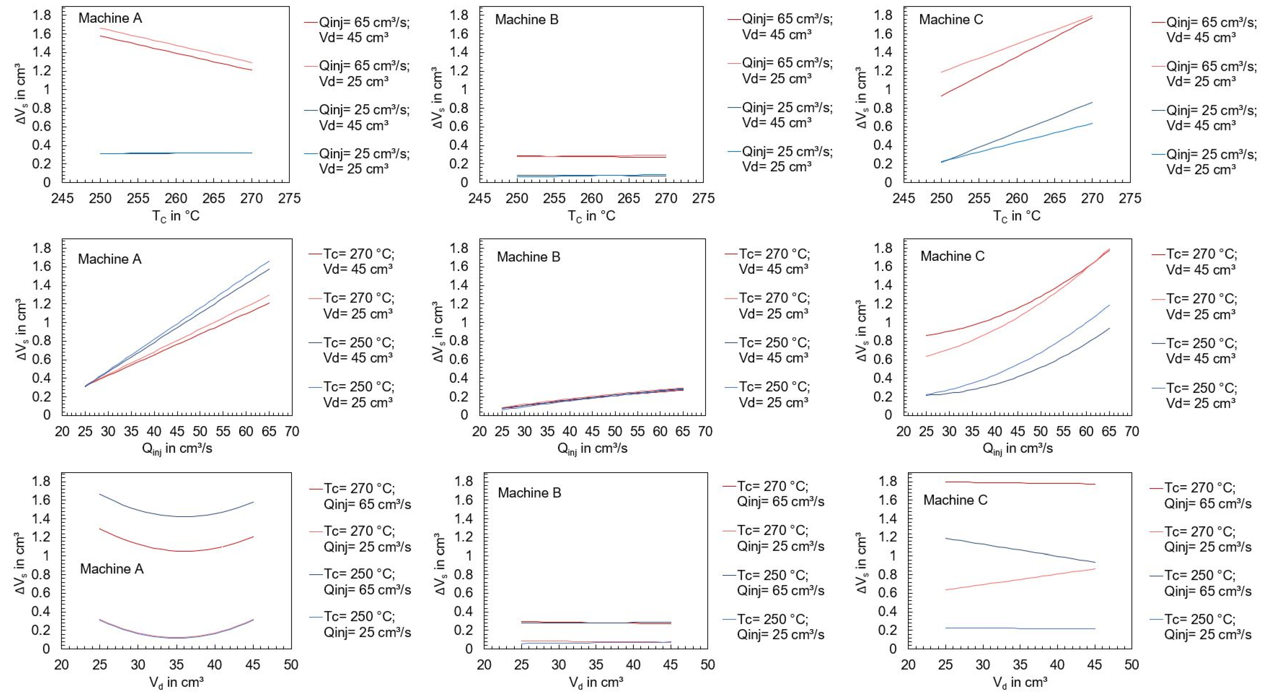
- Variations in the operating points of the machines revealed substantial disparities in the process outcomes, specifically in terms of ejected polymer mass. It has been found that individual changes in the operating point settings have different effects depending on the machine used.
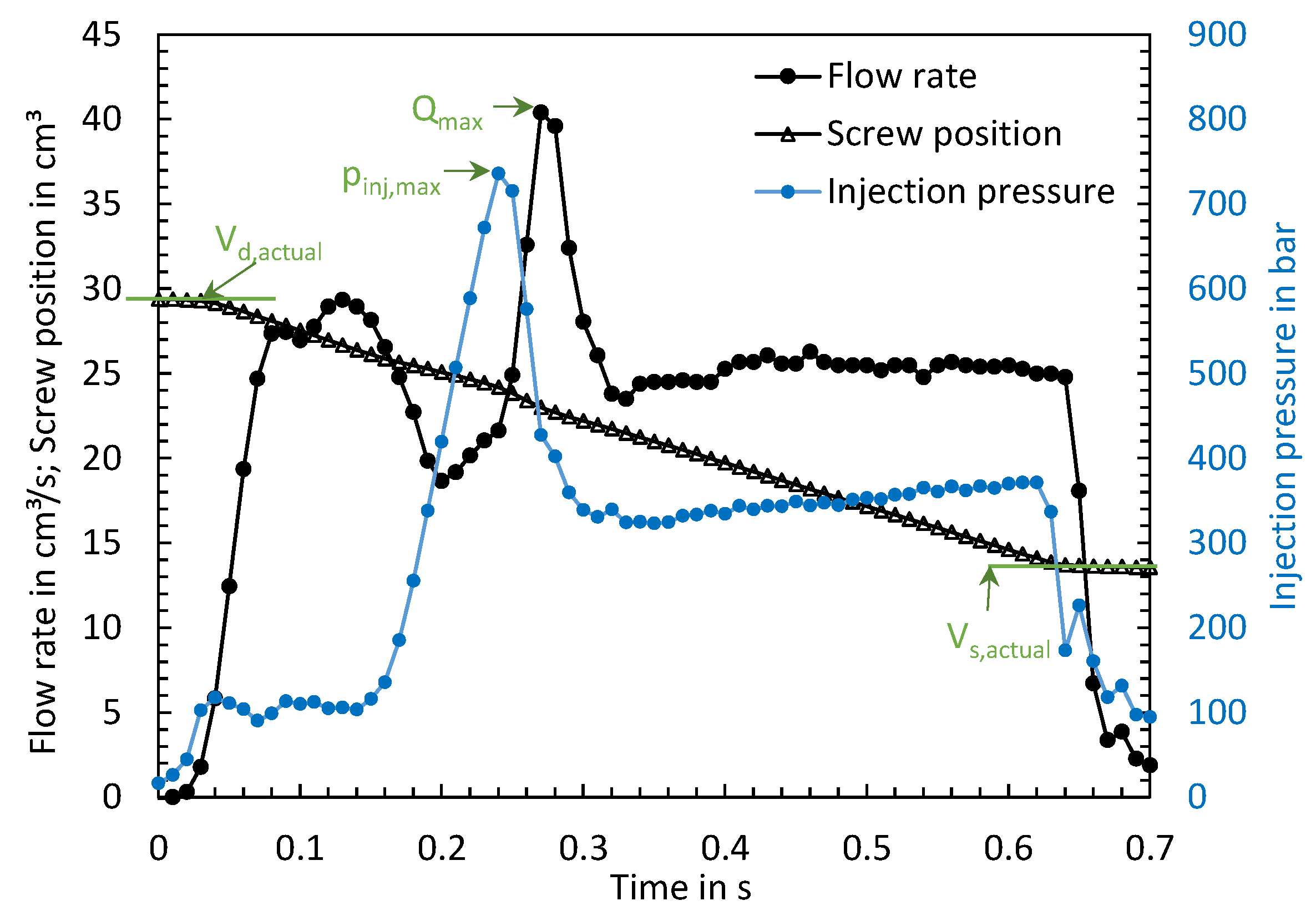
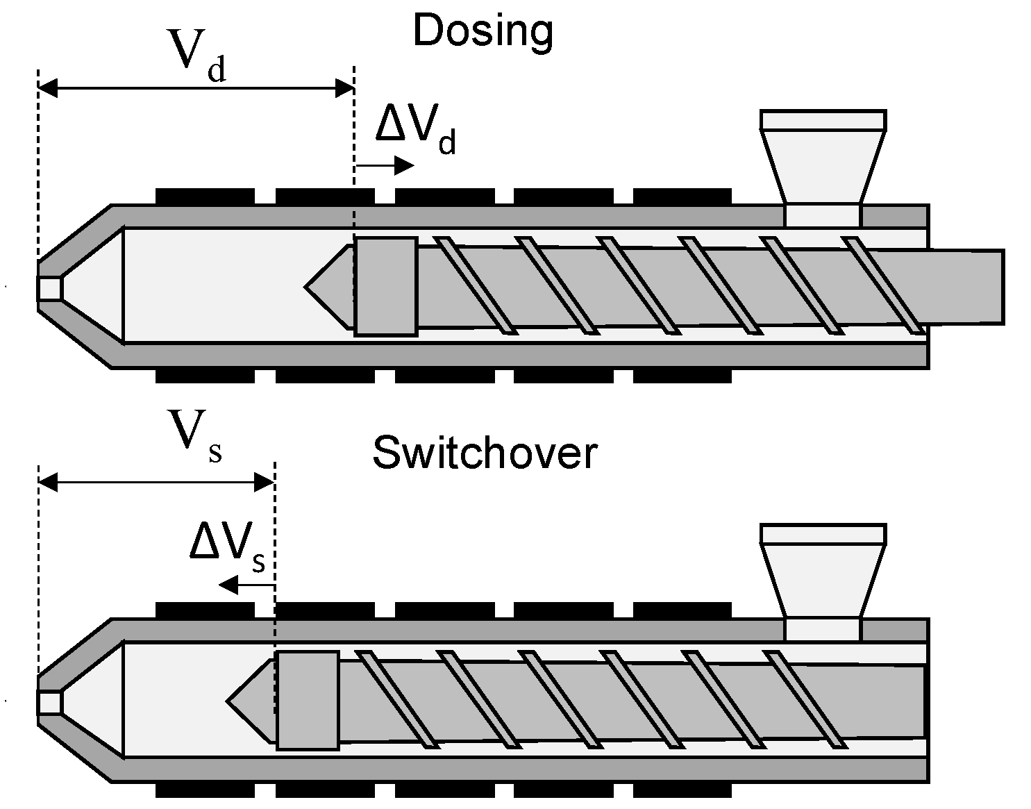
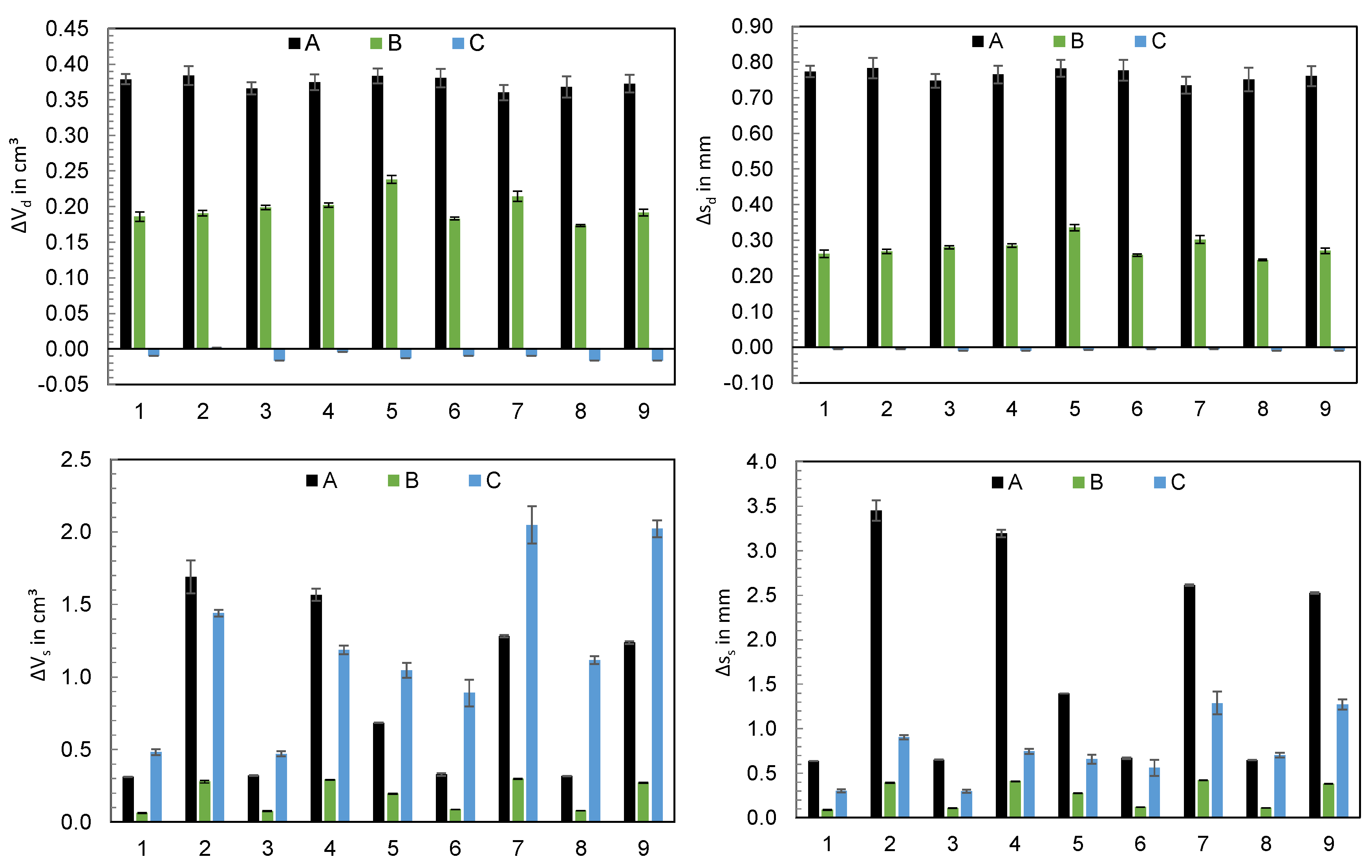
- To elucidate the underlying causes of the substantial disparities in the process outcomes, an evaluation of the measured time series flow rate, injection pressure, and screw position was conducted. By using the time series, the transient behavior of the injection flow rate, the switchover point overrun, and the linearity of the screw’s feed motion was assessed. It was shown that significant differences in the measured time series occur, which can be attributed to the machine, the components of the respective machine, and also the machine setting parameters. Accordingly, the time series of the process parameters offer detailed information for comparing the performance of different machines.
- In order to assess the impact of material characteristics on machine behavior, unreinforced as well as glass fiber-reinforced polyamide was processed on two different hydraulic injection molding machines. The time series of the process parameters have shown that, in addition to the operating point, the material properties also have an effect on the precision of the machine. The machine’s ability to compensate material fluctuations depends on the machine itself. The material-specific influence on the precision of the machine is especially of particular interest in the processing of recycled material, as variations in the material characteristics have different effects on the process. In this context, knowledge about the robustness of the machines to material variations can be very helpful in the selection of the MMMC. For this purpose, the measured time series can be utilized for evaluating the robustness of the machine.
- The above-described occurrences can be responsible for discrepancies between CFD simulation results, which do not account for the machine’s dynamic behavior, and experimental data. This is a crucial consideration, particularly when using simulation data as a substitute for experimental results.
- The thermal start-up behavior of the machines should be characterized in more detail. Here, monitoring of the hydraulic oil temperature, temperature sensors installed in the mold, or measuring sensors in the screw antechamber could potentially be used to identify relevant factors with an impact on the start-up dynamics.
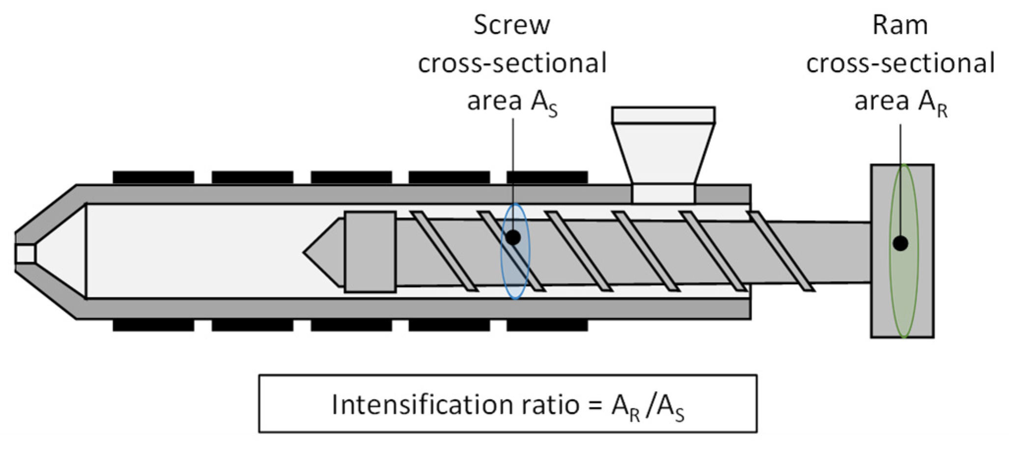
- The high-resolution time series of the process parameters provide a lot of information about the behavior of the machine. The fingerprint should include characteristics describing the machine-dependent dynamics of the process parameters. Characteristic values of the machine control (e.g., of the PID controller) could be used to obtain information on the transient behavior of the injection flow rate or characteristics describing the dynamics of the hydraulics and its components as well as the overrun characteristics of the servo motor. In addition, the IR is an important parameter which provides information about the relationship between hydraulic pressure and pressure in the screw antechamber, and should be taken into account.
- To incorporate the material-specific characteristics of the machines into the fingerprint, reference tests could be established, for example. Using an inline viscosity nozzle (as presented in [32]), the correlations between material properties and process behavior could be examined for generating specific coefficients.
Author Contributions
Funding
Institutional Review Board Statement
Data Availability Statement
Conflicts of Interest
Appendix A

| Machine | Zone 1 (Tc) | Zone 2 | Zone 3 | Zone 4 | Zone 5 | Zone 6 | Zone 7 | Zone 8 |
|---|---|---|---|---|---|---|---|---|
| A | 250 °C | 245 °C | 240 °C | 235 °C | 230 °C | |||
| B | 250 °C | 245 °C | 240 °C | 235 °C | 230 °C | |||
| C | 250 °C | 245 °C | 245 °C | 240 °C | 240 °C | 235 °C | 235 °C | 230 °C |
Regression Models
| Variable | Parameter |
|---|---|
| X1 | Qinj in cm3/s |
| X2 | Vd in cm3 |
| X3 | Tc in °C |
| Machine | Regression | R2 |
|---|---|---|
| A | mass in g = −31.57 + 0.2815 X1 − 0.622 X2 + 0.1927 X3 + 0.001228 X12 − 0.000881 X1 × X2 − 0.001265 X1 × X3 + 0.002732 X2 × X3 | 98.43% |
| B | mass in g = 8.283 + 0.04272 X1 + 0.0727 X2 + 0.01741 X3 − 0.000436 X12 + 0.000120 X1 × X2 − 0.000334 X2 × X3 | 94.65% |
| C | mass in g = 40.41 − 0.2668 X1 − 2.422 X2 − 0.0445 X3 + 0.01180 X22 − 0.000786 X1 × X2 + 0.001287 X1 × X3 + 0.006272 X2 × X3 | 98.16% |
| Machine | Regression | R2 |
|---|---|---|
| A | ΔVs in cm3 = −1.401 + 0.15407 X1 − 0.1357 X2 + 0.01212 X3 + 0.001974 X22 − 0.000103 X1 × X2 − 0.000471 X1 × X3 | 99.38% |
| B | ΔVs in cm3 = −1.1013 + 0.01362 X1 + 0.01990 X2 + 0.003719 X3 − 0.000039 X12 − 0.000013 X1 × X2 − 0.000017 X1 × X3 − 0.000075 X2 × X3 | 99.80% |
| C | ΔVs in cm3 = 0.39 − 0.0654 X1 − 0.1387 X2 − 0.00014 X3 + 0.000402 X12 − 0.000308 X1 × X2 + 0.000244 X1 × X3 + 0.000584 X2 × X3 | 98.84% |
References
- Schut, J.H. Demystifying Energy Saving Devices on Injection Molding Machines. Available online: https://plasticsengineering.wordpress.com/2013/08/31/demystifying-energy-saving-devices-on-injection-molding-machines/ (accessed on 15 October 2023).
- Huang, M.-S.; Nian, S.-C.; Lin, G.-T. Influence of V/P switchover point, injection speed, and holding pressure on quality consistency of injection-molded parts. J. Appl. Polym. Sci. 2021, 138, 51223. [Google Scholar] [CrossRef]
- Chen, J.-Y.; Liu, C.-Y.; Huang, M.-S. Enhancement of Injection Molding Consistency by Adjusting Velocity/Pressure Switching Time Based on Clamping Force. Int. Polym. Process. 2019, 34, 564–572. [Google Scholar] [CrossRef]
- Stemmler, S.; Ay, M.; Vukovic, M.; Abel, D.; Heinisch, J.; Hopmann, C. (Eds.) Cross-Phase Model-Based Predictive Cavity Pressure Control in Injection Molding. In Proceedings of the 3rd IEEE Conference on Control Technology and Applications, City University of Hong Kong, Hong Kong, China, 19–21 August 2019. [Google Scholar]
- Schröder, T. Rheologie der Kunststoffe: Theorie und Praxis, 2nd. ed; aktualisierte und erweiterte Auflage; Hanser: München, Germany, 2020; ISBN 9783446465503. [Google Scholar]
- Middleman, S. Fundamentals of Polymer Processing; McGraw-Hill, Inc.: New York, NY, USA, 1977; ISBN 978-0070418516. [Google Scholar]
- Yao, K.; Gao, F.; Allgöwer, F. Barrel temperature control during operation transition in injection molding. Control Eng. Pract. 2008, 16, 1259–1264. [Google Scholar] [CrossRef]
- Kelly, A.L.; Woodhead, M.; Coates, P.D. Comparison of Injection Molding Machine Performance. Polym. Eng. Sci. 2005, 45, 857–865. [Google Scholar] [CrossRef]
- Bichler, M. Prozessgrössen Beim Spritzgiessen: Analyse und Optimierung; Hüthig: Heidelberg, Germany, 2002; ISBN 3778528440. [Google Scholar]
- Thümen, T. Analyse der Rückstromsperre für den Spritzgießprozess: Prozessoptimierung. Ph.D Thesis, Universität Paderborn, Paderborn, Germany, 2009. [Google Scholar]
- Heinzler, F.A. Modellgestützte Qualitätsregelung durch eine Adaptive, Druckgeregelte Prozessführung beim Spritzgießen. Ph.D Thesis, Universität Duisburg-Essen, Duisburg, Germany, 2014. [Google Scholar]
- Haman, S. Prozessnahes Qualitätsmanagement beim Spritzgießen. Ph.D Thesis, TU Chemnitz, Chemnitz, Germany, 2004. [Google Scholar]
- Kruppa, S. Adaptive Prozessführung und Alternative Einspritzkonzepte beim Spritzgießen von Thermoplasten. Ph.D Thesis, Universität Duisburg-Essen, Duisburg, Germany, 2015. [Google Scholar]
- Eben, J. Identifikation und Reduzierung realer Schwankungen durch Praxistaugliche Prozessführungsmethoden beim Spritzgießen. Ph.D Thesis, Technische Universität Chemnitz, Chemnitz, Germany, 2014. [Google Scholar]
- Shen, C.; Wang, L.; Li, Q. Optimization of injection molding process parameters using combination of artificial neural network and genetic algorithm method. J. Mater. Process. Technol. 2007, 183, 412–418. [Google Scholar] [CrossRef]
- Rosato, D.V.; Rosato, D.V.; Rosato, M.G. Injection Molding Handbook; Springer: Boston, MA, USA, 2000; ISBN 978-1-4613-7077-2. [Google Scholar]
- Chen, W.-C.; Tai, P.-H.; Wang, M.-W.; Deng, W.-J.; Chen, C.-T. A neural network-based approach for dynamic quality prediction in a plastic injection molding process. Expert Syst. Appl. 2008, 35, 843–849. [Google Scholar] [CrossRef]
- Lau, H.C.W.; Ning, A.; Chin, K.S. Neural networks for the dimensional control of molded parts based on a reverse process model. J. Mater. Process. Technol. 2001, 117, 89–96. [Google Scholar] [CrossRef]
- Manjunath, P.G.; Krishna, P. Prediction and Optimization of Dimensional Shrinkage Variations in Injection Molded Parts Using Forward and Reverse Mapping of Artificial Neural Networks. AMR 2012, 463-464, 674–678. [Google Scholar] [CrossRef]
- Li, E.; Jia, L.; Yu, J. A genetic neural fuzzy system-based quality prediction model for injection process. Comput. Chem. Eng. 2002, 26, 1253–1263. [Google Scholar] [CrossRef]
- Ribeiro, B. Support Vector Machines for Quality Monitoring in a Plastic Injection Molding Process. IEEE Trans. Syst. Man Cybern. C 2005, 35, 401–410. [Google Scholar] [CrossRef]
- Zhou, X.; Zhang, Y.; Mao, T.; Zhou, H. Monitoring and dynamic control of quality stability for injection molding process. J. Mater. Process. Technol. 2017, 249, 358–366. [Google Scholar] [CrossRef]
- Bogedale, L.; Doerfel, S.; Schrodt, A.; Heim, H.-P. Online Prediction of Molded Part Quality in the Injection Molding Process Using High-Resolution Time Series. Polymers 2023, 15, 978. [Google Scholar] [CrossRef] [PubMed]
- Rehmer, A.; Klute, M.; Kroll, A.; Heim, H.-P. A Digital Twin for Part Quality Prediction and Control in Plastic Injection Molding. Modeling, Identification, and Control for Cyber-Physical Systems Towards Industry 4.0. Available online: https://www.uni-kassel.de/forschung/digital-twin-of-injection-molding/publikationen (accessed on 16 December 2023).
- Rehmer, A.; Klute, M.; Kroll, A.; Heim, H.-P. An internal dynamics approach to predicting batch-end product quality in plastic injection molding using Recurrent Neural Networks. In Proceedings of the 2022 IEEE Conference on Control Technology and Applications, Trieste, Italy, 22–25 August 2022; pp. 1427–1432. [Google Scholar]
- Gim, J.; Yang, H.; Turng, L.-S. Transfer learning of machine learning models for multi-objective process optimization of a transferred mold to ensure efficient and robust injection molding of high surface quality parts. J. Manuf. Process. 2023, 87, 11–24. [Google Scholar] [CrossRef]
- Lockner, Y.; Hopmann, C.; Zhao, W. Transfer learning with artificial neural networks between injection molding processes and different polymer materials. J. Manuf. Process. 2022, 73, 395–408. [Google Scholar] [CrossRef]
- Finkeldey, F.; Volke, J.; Zarges, J.-C.; Heim, H.-P.; Wiederkehr, P. Learning quality characteristics for plastic injection molding processes using a combination of simulated and measured data. J. Manuf. Process. 2020, 60, 134–143. [Google Scholar] [CrossRef]
- DIN EN ISO 527-2; Kunststoffe—Bestimmung der Zugeigenschaften—Teil2: Prüfbedingungen für Form und Extrusionsmassen. Beuth Verlag: Berlin, Germany, 2012.
- Volke, J.; Heim, H.-P. Evaluation of the injection molding process behavior during start-up and after parameter changes using dynamic time warping correspondences. J. Manuf. Process. 2023, 95, 183–203. [Google Scholar] [CrossRef]
- Kulkarni, S. Robust Process Development and Scientific Molding: Theory and Practice, 2nd ed.; Carl Hanser: Munich, Germany, 2017; ISBN 9781569905869. [Google Scholar]
- Zarges, J.-C.; Sälzer, P.; Feldmann, M.; Heim, H.-P. Determining Viscosity Directly in the Injection Molding Process: In-line Rheometer for Natural-Fiber-Reinforced Plastics. Kunststoffe Int. 2016, 10, 106–109. [Google Scholar]
- Chicco, D.; Warrens, M.J.; Jurman, G. The coefficient of determination R-squared is more informative than SMAPE, MAE, MAPE, MSE and RMSE in regression analysis evaluation. PeerJ Comput. Sci. 2021, 7, e623. [Google Scholar] [CrossRef] [PubMed]


| Part | IMM | Materials | Mold | Machine Setup | Focus |
|---|---|---|---|---|---|
| A | A, B, and C | Unfilled polyamide (PA) | Closed | Constant operating point | Influence of the machine on the process result during start-up |
| B | A, B, and C | Unfilled polyamide (PA) | Closed | Variation in nine operating points | Influence of the machine at varying operating points |
| C | A and B | Unfilled (PA) and glass fiber-reinforced polyamide (PAGF30) | Closed and open (injection into atmosphere) | Variation in eight operating points | Influence of the material and mold |
| A | B | C | |
|---|---|---|---|
| Clamping force, kN | 500 | 1100 | 1500 |
| Max. injection flow rate, cm3/s | 66 | 136 | 174 |
| Screw diameter dscrew, mm | 25 | 30 | 45 |
| Nozzle diameter, mm | 4 | 3 | 3 |
| Max. injection pressure, bar | 2500 | 2000 | 2470 |
| Calculated stroke volume, cm3 | 59 | 85 | 318 |
| Effective screw length (length/diameter), - | 24 | 20 | 22 |
| Drive, - | HM | EM | |
| Designation | Qinj, cm3/s | Vd, cm3 | Vs, cm3 | Tc, °C |
|---|---|---|---|---|
| 0 | 45 | 35 | 24 | 260 |
| Designation | Qinj, cm3/s | Vd, cm3 | Vs, cm3 | Tc, °C |
|---|---|---|---|---|
| 1 | 25 | 25 | 14 | 250 |
| 2 | 65 | 25 | 14 | 250 |
| 3 | 25 | 45 | 34 | 250 |
| 4 | 65 | 45 | 34 | 250 |
| 5 | 45 | 35 | 24 | 260 |
| 6 | 25 | 25 | 14 | 270 |
| 7 | 65 | 25 | 14 | 270 |
| 8 | 25 | 45 | 34 | 270 |
| 9 | 65 | 45 | 34 | 270 |
| Designation | Qinj, cm3/s | Vd, cm3 | Vs, cm3 | Tc, °C |
|---|---|---|---|---|
| 1 | 25 | 30.5 | 12.5 | 250 |
| 2 | 25 | 50.5 | 32.5 | 250 |
| 3 | 60 | 30.5 | 12.5 | 250 |
| 4 | 60 | 50.5 | 32.5 | 250 |
| 5 | 25 | 30.5 | 12.5 | 270 |
| 6 | 25 | 50.5 | 32.5 | 270 |
| 7 | 60 | 30.5 | 12.5 | 270 |
| 8 | 60 | 50.5 | 32.5 | 270 |
| Parameter | Parts A and B | Part C |
|---|---|---|
| Screw peripheral speed, m/min | 18 | 15 |
| Back pressure, bar | 60 | 75 |
| Decompression volume, cm3 | 4 | 2 |
| Mold temperature, °C | 75 | 60 |
| Cooling time (with cavity), s | 15 | 30 |
| PA | PAGF30 | |
|---|---|---|
| Trade name | Ultramid B3S | Ultramid B3EG6 |
| Glass fiber ratio, % | 0 | 30 |
| Melt volume rate, cm3/10 min | 160 | 35 |
| Density, g/cm3 | 1.13 | 1.36 |
| Tensile modulus, MPa | 3500 | 9500 |
| Breaking elongation, % | 4 | 3.5 |
Disclaimer/Publisher’s Note: The statements, opinions and data contained in all publications are solely those of the individual author(s) and contributor(s) and not of MDPI and/or the editor(s). MDPI and/or the editor(s) disclaim responsibility for any injury to people or property resulting from any ideas, methods, instructions or products referred to in the content. |
© 2023 by the authors. Licensee MDPI, Basel, Switzerland. This article is an open access article distributed under the terms and conditions of the Creative Commons Attribution (CC BY) license (https://creativecommons.org/licenses/by/4.0/).
Share and Cite
Knoll, J.; Heim, H.-P. Analysis of the Machine-Specific Behavior of Injection Molding Machines. Polymers 2024, 16, 54. https://doi.org/10.3390/polym16010054
Knoll J, Heim H-P. Analysis of the Machine-Specific Behavior of Injection Molding Machines. Polymers. 2024; 16(1):54. https://doi.org/10.3390/polym16010054
Chicago/Turabian StyleKnoll, Julia, and Hans-Peter Heim. 2024. "Analysis of the Machine-Specific Behavior of Injection Molding Machines" Polymers 16, no. 1: 54. https://doi.org/10.3390/polym16010054
APA StyleKnoll, J., & Heim, H.-P. (2024). Analysis of the Machine-Specific Behavior of Injection Molding Machines. Polymers, 16(1), 54. https://doi.org/10.3390/polym16010054