
Effect of Surface Contamination on Near-Infrared Spectra of Biodegradable Plastics

 , ,
, ,  , and
, and
Abstract

1. Introduction
2. Materials and Methods
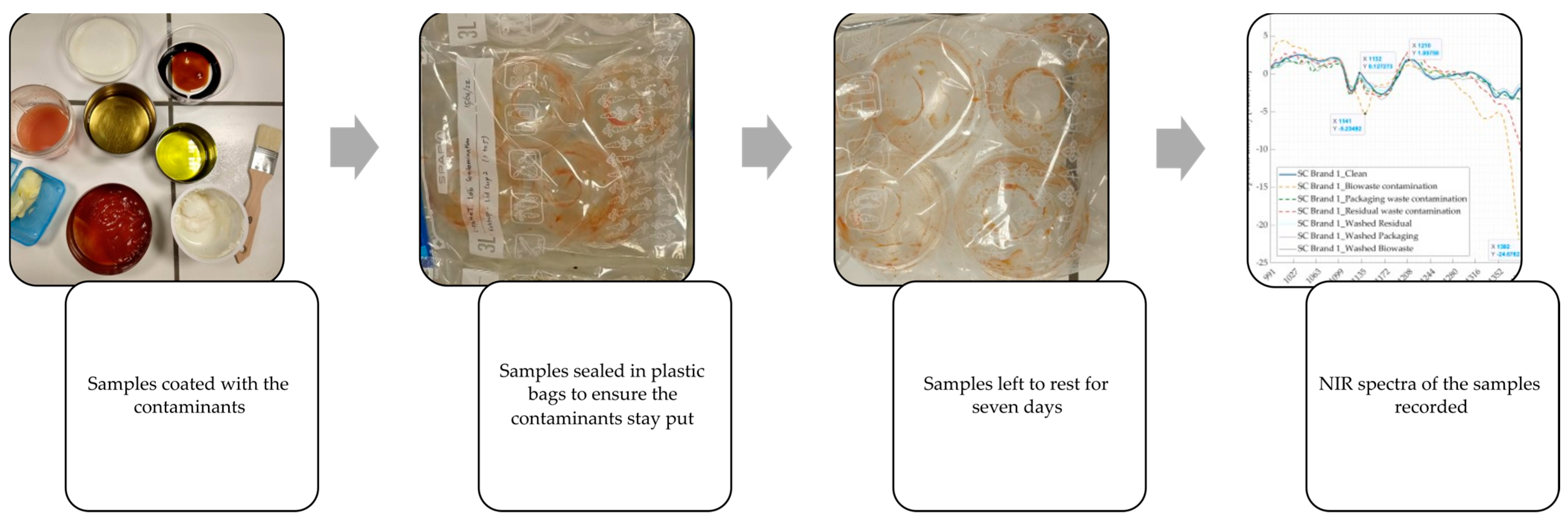
2.1. Experiment 1: Artificially Induced Contamination under Laboratory Conditions
2.1.1. Samples, Used Contaminants, and Sample Preparation
2.1.2. Equipment Used as Well as Recording and Processing of Spectra
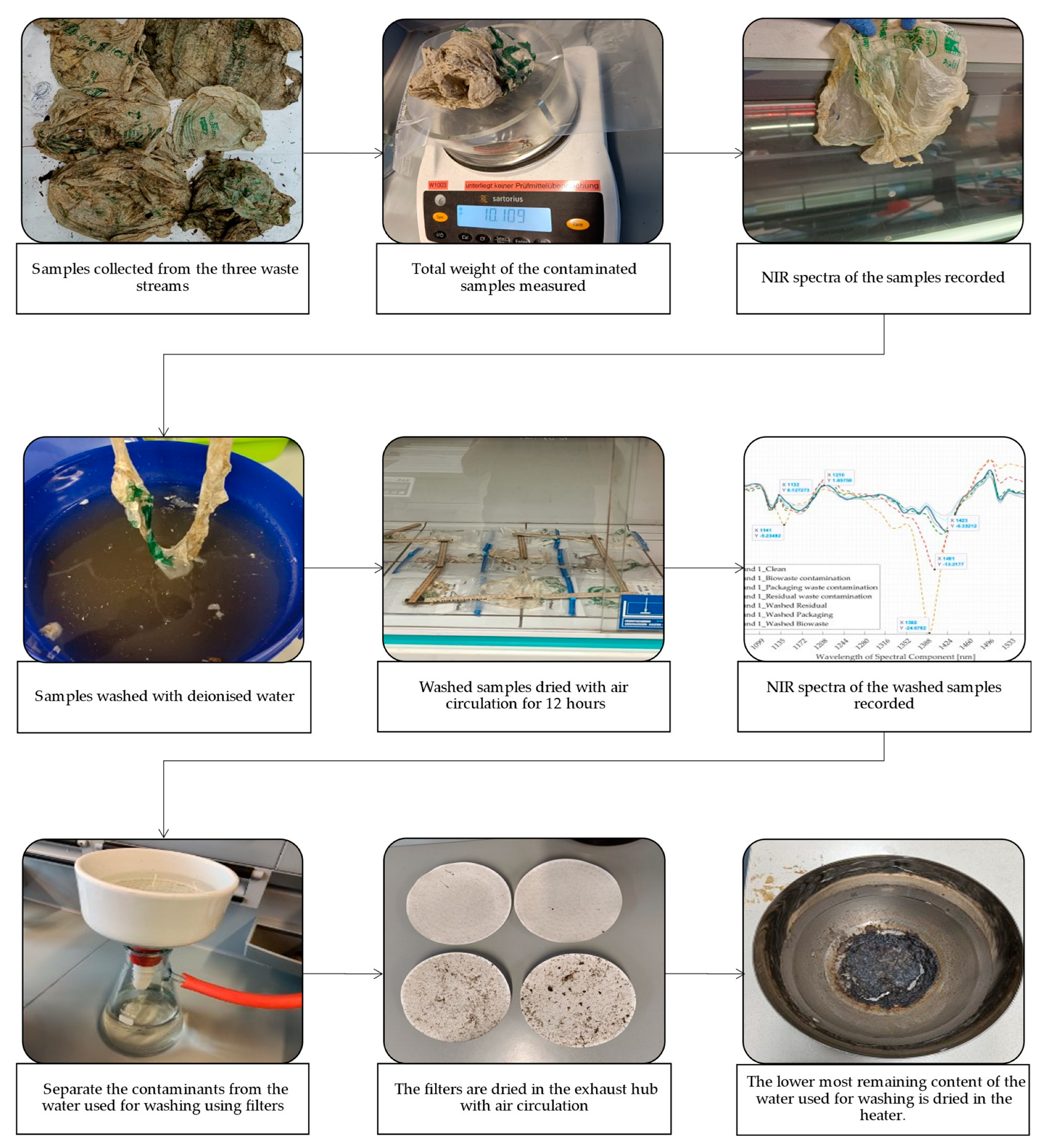
2.2. Experiment 2: Real-World Contaminated Samples from the Three Waste Streams
2.2.1. Sampling of Items and Sample Preparation
2.2.2. Equipment Used as Well as Recording and Processing of Spectra
3. Results and Discussion
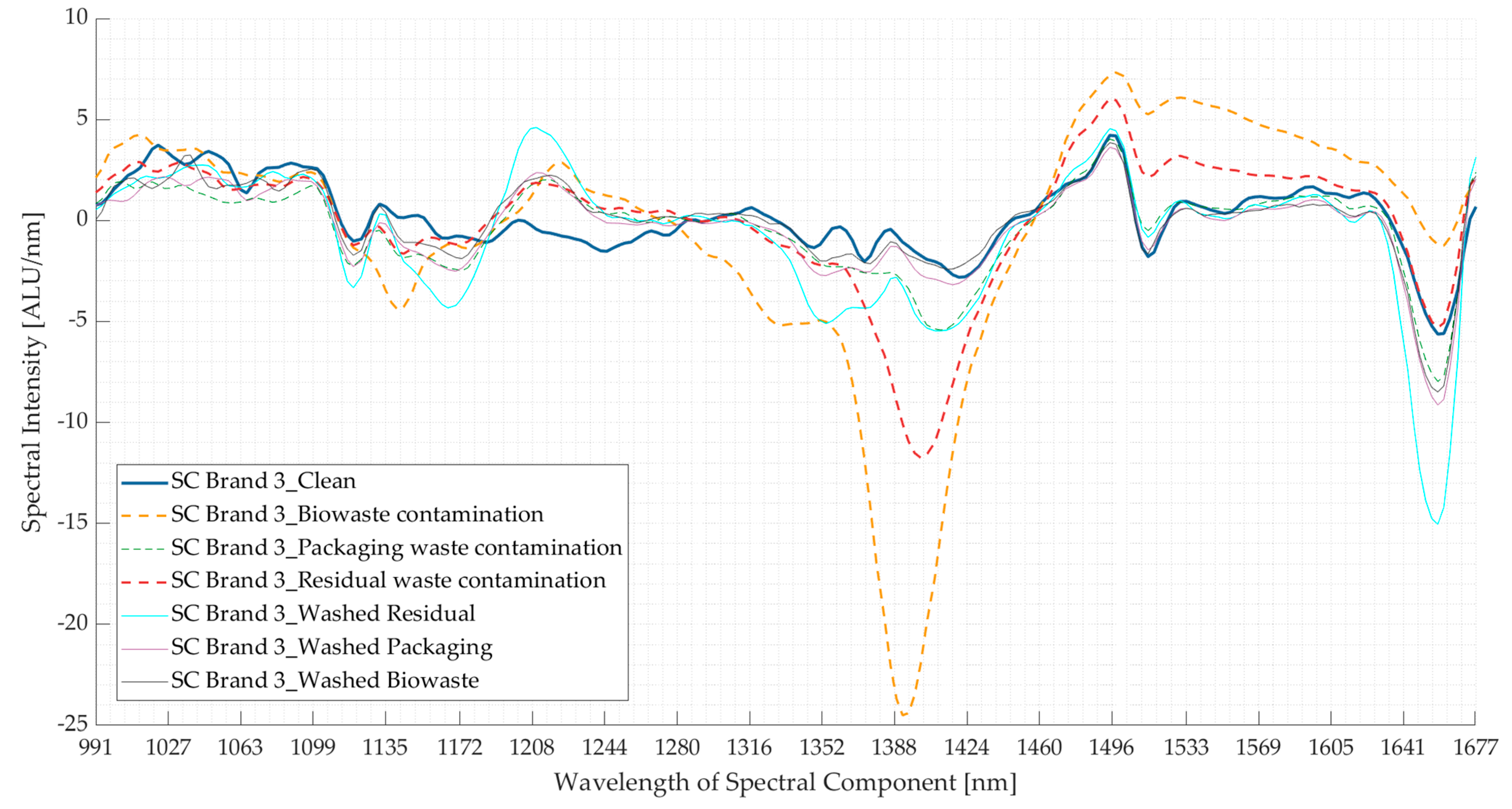
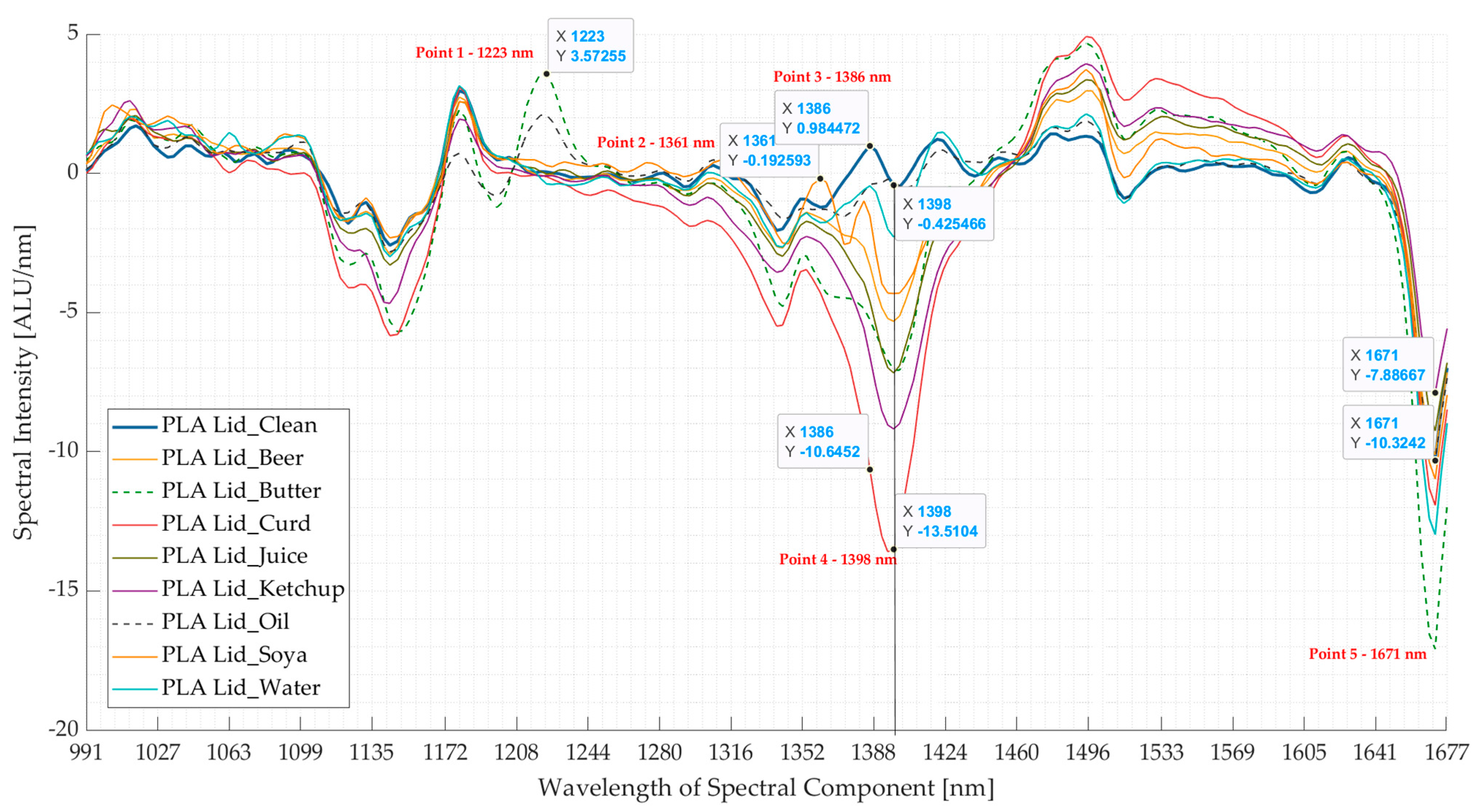
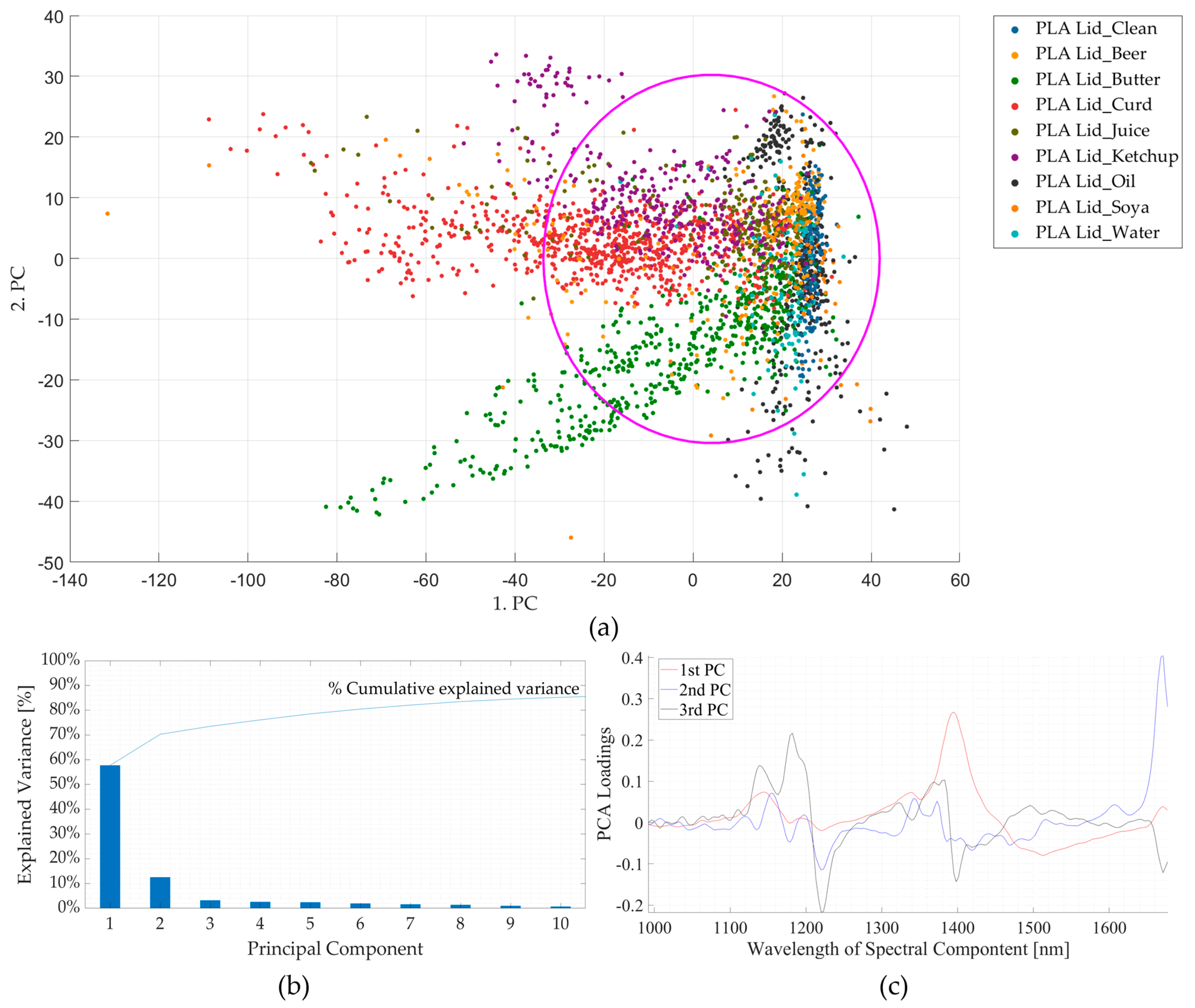
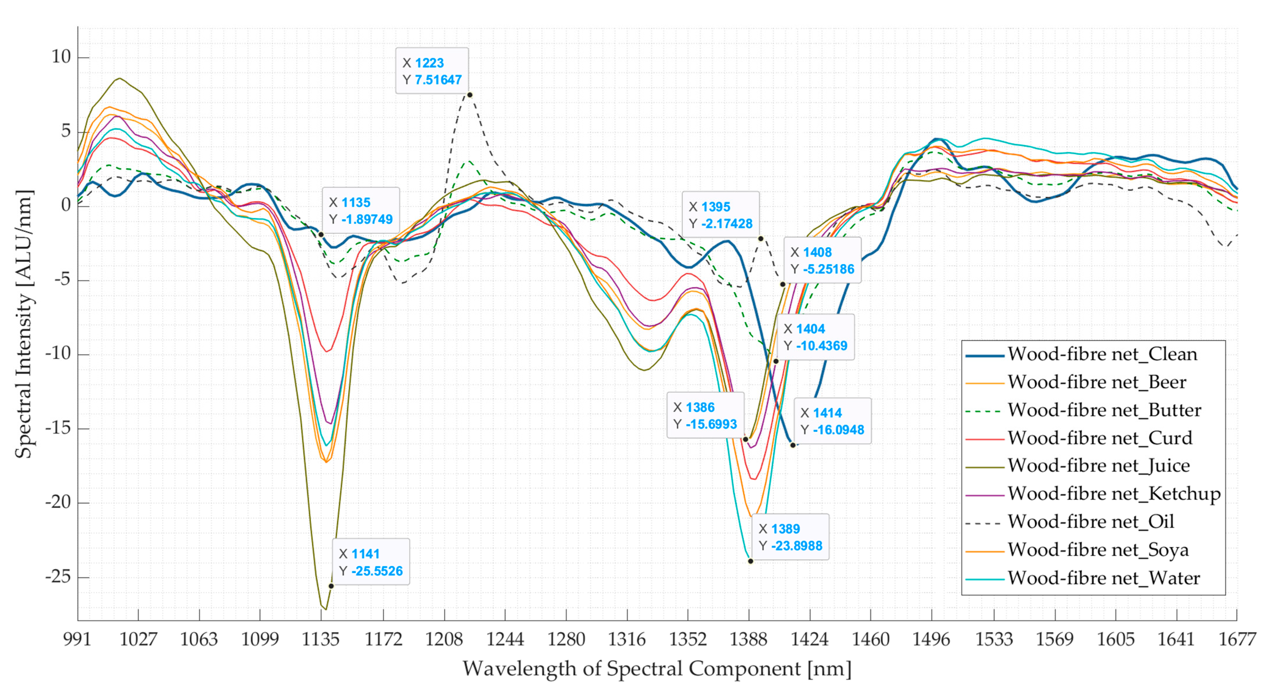
3.1. Experiment 1: Artificially Induced Contamination Using Food-Derived Contaminants
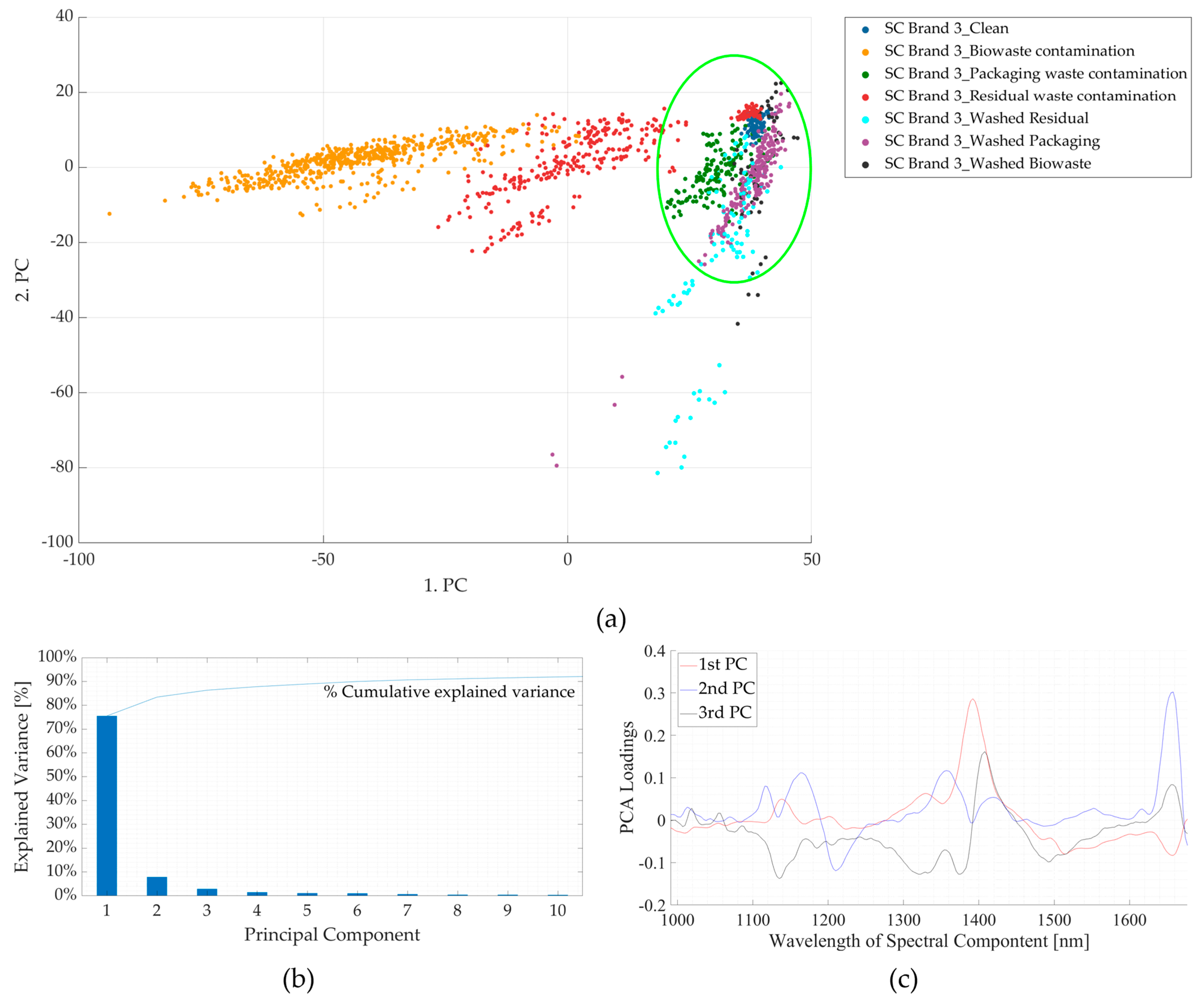
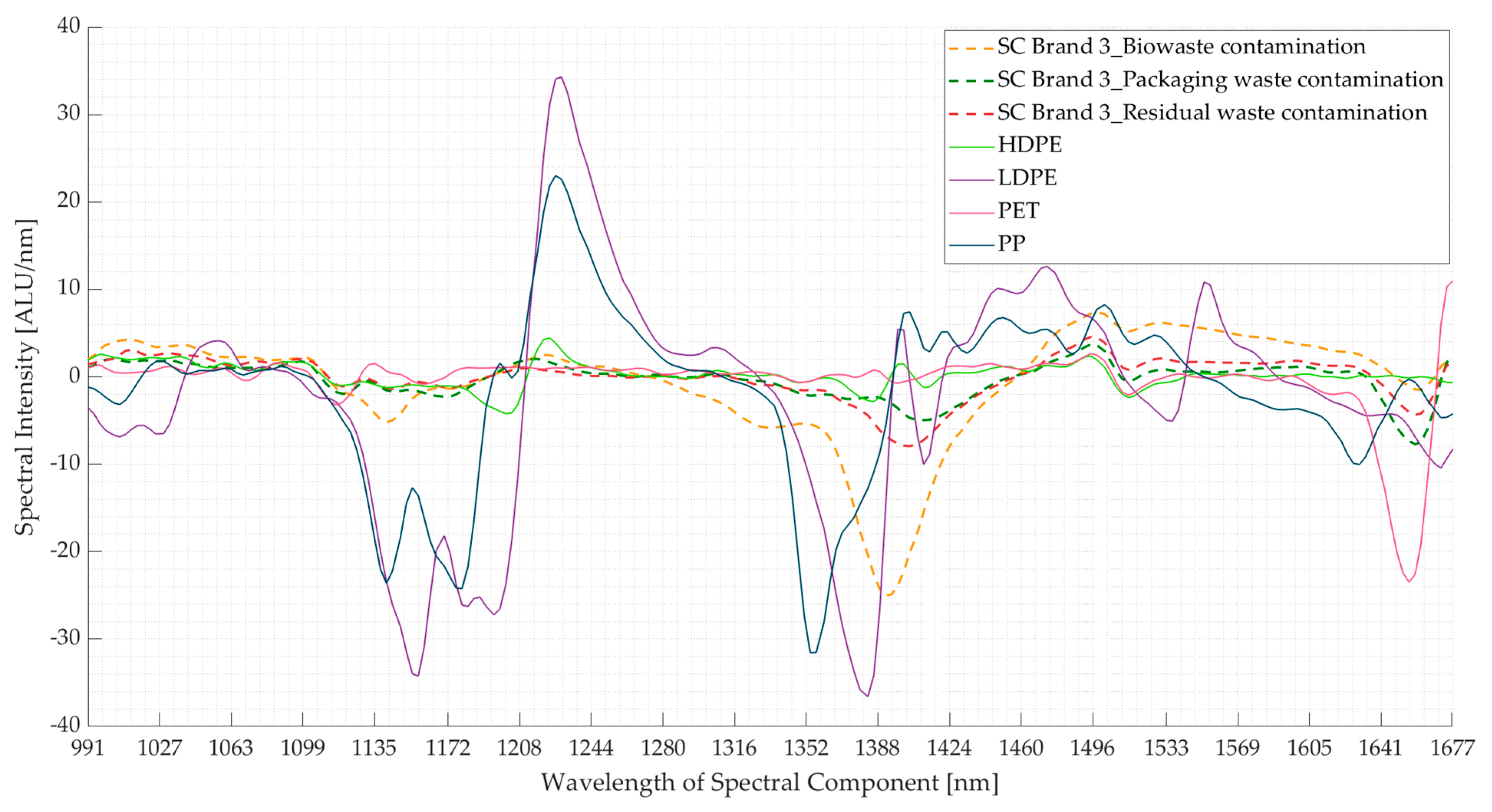
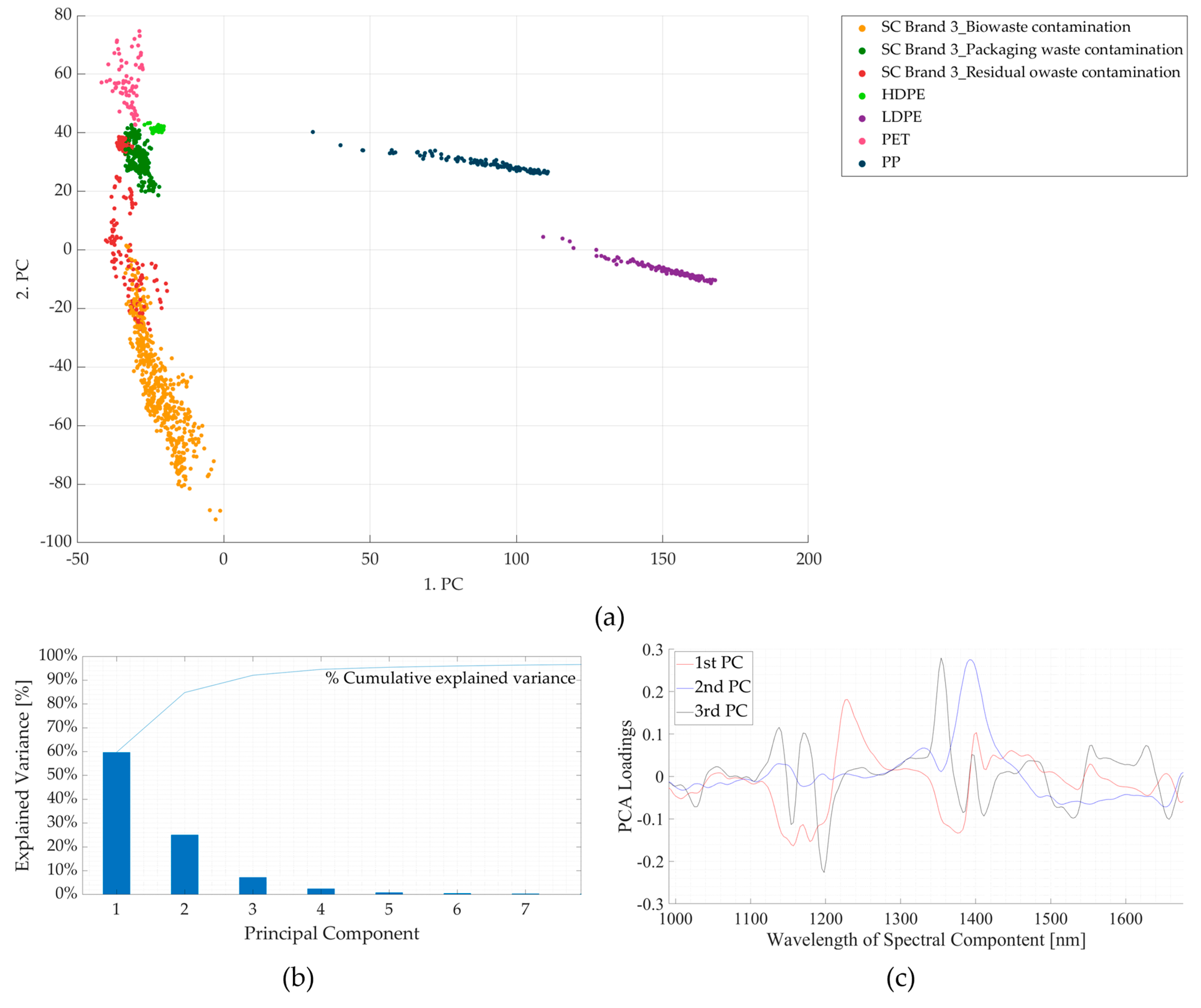
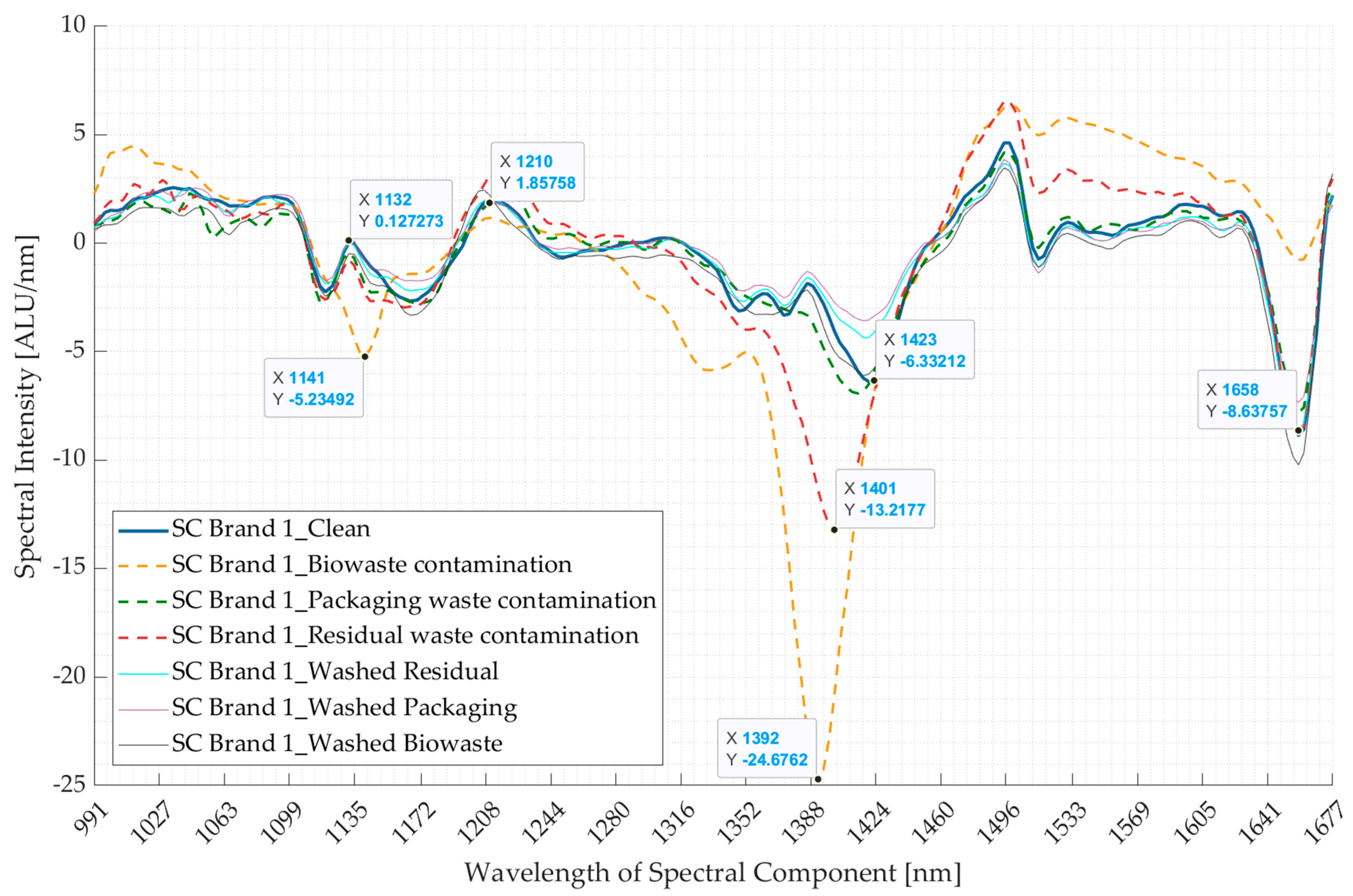
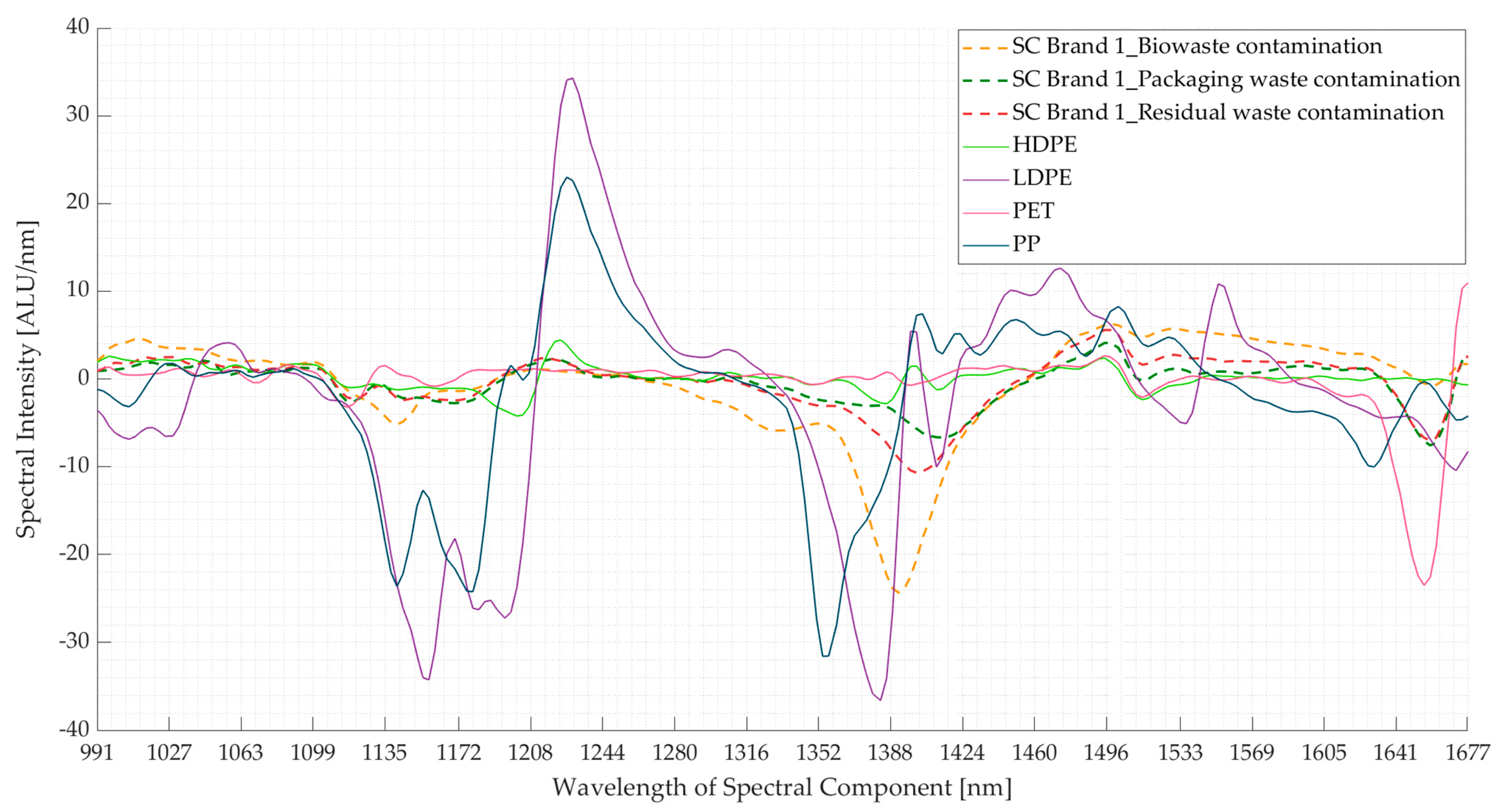
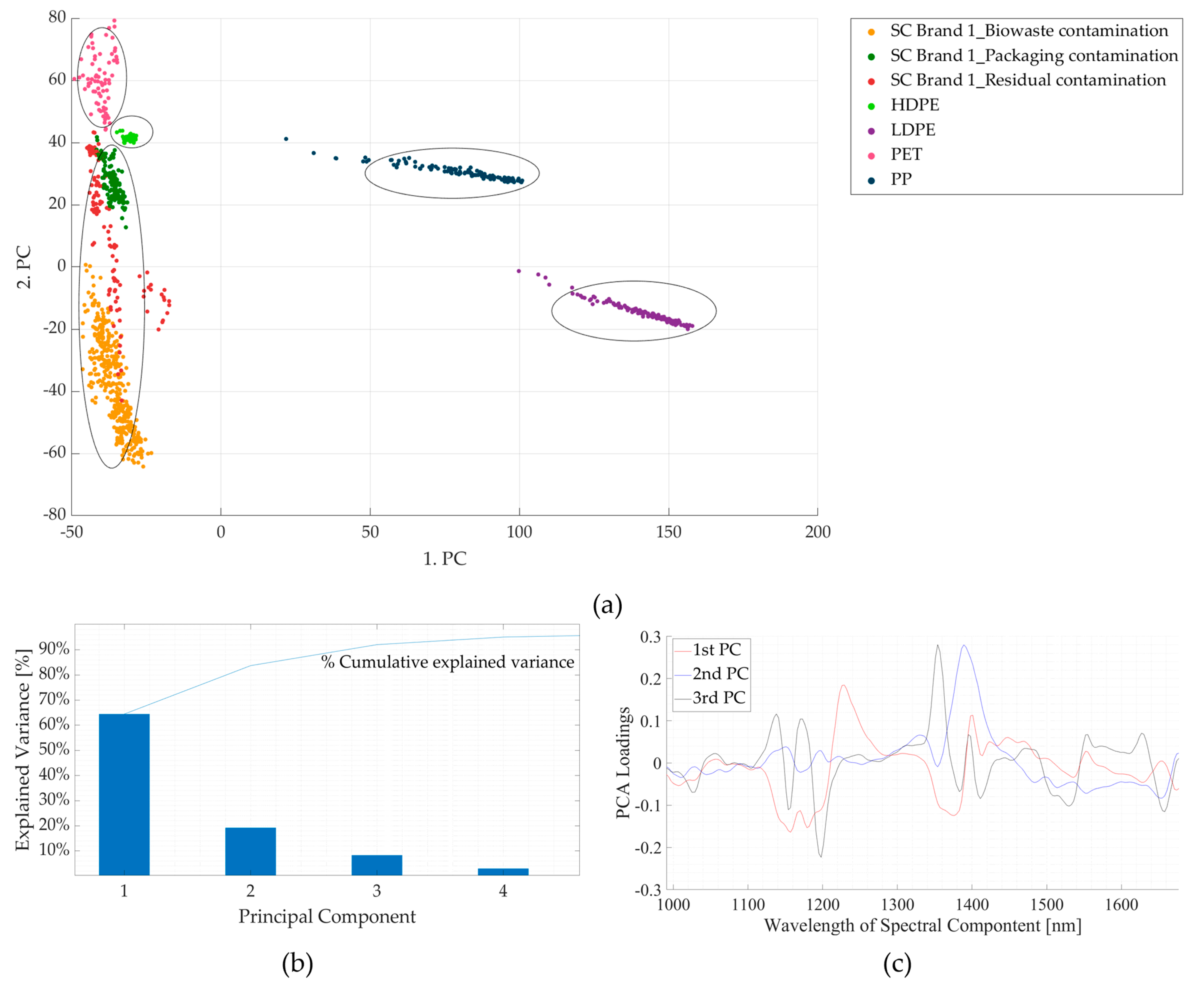
3.2. Experiment 2: Contaminated Samples from the Three Waste Streams
4. Conclusions
Author Contributions
Funding
Institutional Review Board Statement
Data Availability Statement
Conflicts of Interest
Appendix A
References
- Niaounakis, M. Recycling of biopolymers—The patent perspective. Eur. Polym. J. 2019, 114, 464–475. [Google Scholar] [CrossRef]
- Hottle, T.A.; Bilec, M.M.; Landis, A.E. Sustainability assessments of bio-based polymers. Polym. Degrad. Stab. 2013, 98, 1898–1907. [Google Scholar] [CrossRef]
- Döhler, N.; Wellenreuther, C.; Wolf, A. Market dynamics of biodegradable bio-based plastics: Projections and linkages to European policies. EFB Bioeconomy J. 2022, 2, 100028. [Google Scholar] [CrossRef]
- Castro-Aguirre, E.; Iñiguez-Franco, F.; Samsudin, H.; Fang, X.; Auras, R. Poly(lactic acid)-Mass production, processing, industrial applications, and end of life. Adv. Drug Deliv. Rev. 2016, 107, 333–366. [Google Scholar] [CrossRef]
- European Bioplastics, e.V. Bioplastics Market Development Update 2023: Growth Resumption: Global Production Capacities of Bioplastics 2023–2028. Available online: https://www.european-bioplastics.org/market/ (accessed on 13 February 2024).
- Communication from the Commission to the European Parliament, the Council, the European Economic and Social Committee and the Committee of the regions: EU policy framework on biobased, biodegradable and compostable plastics. 2022.
- Al-Salem, S.M.; Lettieri, P.; Baeyens, J. Recycling and recovery routes of plastic solid waste (PSW): A review. Waste Manag. 2009, 29, 2625–2643. [Google Scholar] [CrossRef]
- Ruj, B.; Pandey, V.; Jash, P.; Srivastava, V.K. Sorting of plastic waste for effective recycling. Int. J. Appl. Sci. Eng. Res. 2015, 4, 564–571. [Google Scholar]
- Bonifazi, G.; Gasbarrone, R.; Serranti, S. DETECTING CONTAMINANTS IN POST-CONSUMER PLASTIC PACKAGING WASTE BY A NIR HYPER-SPECTRAL IMAGING-BASED CASCADE DETECTION APPROACH. Detritus 2021, 15, 94–106. [Google Scholar] [CrossRef]
- Wedin, H.; Gupta, C.; Mzikian, P.; Englund, F.; Hornbuckle, R.; Troppenz, V.; Kobal, L.; Costi, M.; Ellams, D.; Olsson, S. Can automated NIR technology be a way to improve the sorting quality of textile waste? In Environmental Science, Materials Science, Engineering; Research Institutes of Sweden: Gothenburg, Sweden, 2017. [Google Scholar]
- Koinig, G.; Friedrich, K.; Rutrecht, B.; Oreski, G.; Barretta, C.; Vollprecht, D. Influence of reflective materials, emitter intensity and foil thickness on the variability of near-infrared spectra of 2D plastic packaging materials. Waste Manag. 2022, 144, 543–551. [Google Scholar] [CrossRef]
- Yang, J.; Xu, Y.-P.; Chen, P.; Li, J.-Y.; Liu, D.; Chu, X.-L. Combining spectroscopy and machine learning for rapid identification of plastic waste: Recent developments and future prospects. J. Clean. Prod. 2023, 431, 139771. [Google Scholar] [CrossRef]
- Küppers, B.; Schloegl, S.; Oreski, G.; Pomberger, R.; Vollprecht, D. Influence of surface roughness and surface moisture of plastics on sensor-based sorting in the near infrared range. Waste Manag. Res. 2019, 37, 843–850. [Google Scholar] [CrossRef]
- Masoumi, H.; Safavi, S.M.; Khani, Z. Identification and classification of plastic resins using near infrared reflectance spectroscopy. Int. J. Mech. Ind. Eng. 2012, 6, 213–220. [Google Scholar]
- Zou, H.-H.; He, P.-J.; Peng, W.; Lan, D.-Y.; Xian, H.-Y.; Lü, F.; Zhang, H. Rapid detection of colored and colorless macro- and micro-plastics in complex environment via near-infrared spectroscopy and machine learning. J. Environ. Sci. 2024, 147, 512–522. [Google Scholar] [CrossRef]
- Eriksen, M.K.; Damgaard, A.; Boldrin, A.; Astrup, T.F. Quality Assessment and Circularity Potential of Recovery Systems for Household Plastic Waste. J. Ind. Ecol. 2019, 23, 156–168. [Google Scholar] [CrossRef]
- Bassey, U.; Rojek, L.; Hartmann, M.; Creutzburg, R.; Volland, A. The potential of NIR spectroscopy in the separation of plastics for pyrolysis. Electron. Imaging 2021, 33, 143-1–143-14. [Google Scholar] [CrossRef]
- Ji, T.; Fang, H.; Zhang, R.; Yang, J.; Fan, L.; Hu, Y.; Cai, Z. Low-value recyclable waste identification based on NIR feature analysis and RGB-NIR fusion. Infrared Phys. Technol. 2023, 131, 104693. [Google Scholar] [CrossRef]
- Kakadellis, S.; Harris, Z.M. Don’t scrap the waste: The need for broader system boundaries in bioplastic food packaging life-cycle assessment—A critical review. J. Clean. Prod. 2020, 274, 122831. [Google Scholar] [CrossRef]
- Kakadellis, S.; Woods, J.; Harris, Z.M. Friend or foe: Stakeholder attitudes towards biodegradable plastic packaging in food waste anaerobic digestion. Resour. Conserv. Recycl. 2021, 169, 105529. [Google Scholar] [CrossRef]
- Cazaudehore, G.; Guyoneaud, R.; Evon, P.; Martin-Closas, L.; Pelacho, A.M.; Raynaud, C.; Monlau, F. Can anaerobic digestion be a suitable end-of-life scenario for biodegradable plastics? A critical review of the current situation, hurdles, and challenges. Biotechnol. Adv. 2022, 56, 107916. [Google Scholar] [CrossRef] [PubMed]
- Bátori, V.; Åkesson, D.; Zamani, A.; Taherzadeh, M.J.; Sárvári Horváth, I. Anaerobic degradation of bioplastics: A review. Waste Manag. 2018, 80, 406–413. [Google Scholar] [CrossRef] [PubMed]
- Fredi, G.; Dorigato, A. Recycling of bioplastic waste: A review. Adv. Ind. Eng. Polym. Res. 2021, 4, 159–177. [Google Scholar] [CrossRef]
- Ciriminna, R.; Pagliaro, M. Biodegradable and Compostable Plastics: A Critical Perspective on the Dawn of their Global Adoption. ChemistryOpen 2020, 9, 8–13. [Google Scholar] [CrossRef]
- Rossi, V.; Cleeve-Edwards, N.; Lundquist, L.; Schenker, U.; Dubois, C.; Humbert, S.; Jolliet, O. Life cycle assessment of end-of-life options for two biodegradable packaging materials: Sound application of the European waste hierarchy. J. Clean. Prod. 2015, 86, 132–145. [Google Scholar] [CrossRef]
- Mhaddolkar, N.; Koinig, G.; Vollprecht, D. NEAR-INFRARED IDENTIFICATION AND SORTING OF POLYLACTIC ACID. Detritus 2022, 20, 29–40. [Google Scholar] [CrossRef]
- Mhaddolkar, N.; Vollprecht, D. Evaluation of a near-infrared sorting system for bio-based and biodegradable plastics. In Proceedings of the 11. Wissenschaftskongress Abfall-und Ressourcenwirtschaft, Dresden, Germany, 16–18 March 2022. [Google Scholar]
- Chen, X.; Kroell, N.; Li, K.; Feil, A.; Pretz, T. Influences of bioplastic polylactic acid on near-infrared-based sorting of conventional plastic. Waste Manag. Res. 2021, 39, 1113–1213. [Google Scholar] [CrossRef] [PubMed]
- Handschick, B.; Wohllebe, M.; Hollstein, F. Möglichkeiten und Grenzen der Sortierung von Biokunststoffen mit neuer NIR Sortiertechnik. In Proceedings of the Biokunststoffe in Verwertung und Recycling, Dresden, Germany, 3–4 December 2012. [Google Scholar]
- Ulrici, A.; Serranti, S.; Ferrari, C.; Cesare, D.; Foca, G.; Bonifazi, G. Efficient chemometric strategies for PET–PLA discrimination in recycling plants using hyperspectral imaging. Chemom. Intell. Lab. Syst. 2013, 122, 31–39. [Google Scholar] [CrossRef]
- Friedrich, K.; Koinig, G.; Pomberger, R.; Vollprecht, D. Qualitative analysis of post-consumer and post-industrial waste via near-infrared, visual and induction identification with experimental sensor-based sorting setup. MethodsX 2022, 9, 101686. [Google Scholar] [CrossRef] [PubMed]
- ASTM Standardization News. Biobased Labeling Connects in ASTM Certification. Available online: https://sn.astm.org/?q=features/biobased-labeling-connects-astm-certification-mj11.html (accessed on 11 August 2022).
- Mhaddolkar, N.; Tischberger-Aldrian, A.; Astrup, T.F.; Vollprecht, D. Consumers confused ‘Where to dispose biodegradable plastics?’: A study of three waste streams. Waste Manag. Res. 2024, 1–12. [Google Scholar] [CrossRef] [PubMed]
- Bastioli, C. Properties and applications of Mater-Bi starch-based materials. Polym. Degrad. Stab. 1998, 59, 263–272. [Google Scholar] [CrossRef]
- Cayuela, J.A.; García, J.F. Sorting olive oil based on alpha-tocopherol and total tocopherol content using near-infra-red spectroscopy (NIRS) analysis. J. Food Eng. 2017, 202, 79–88. [Google Scholar] [CrossRef]
- Gislum, R.; Nikneshan, P.; Shrestha, S.; Tadayyon, A.; Deleuran, L.; Boelt, B. Characterisation of Castor (Ricinus communis L.) Seed Quality Using Fourier Transform Near-Infrared Spectroscopy in Combination with Multivariate Data Analysis. Agriculture 2018, 8, 59. [Google Scholar] [CrossRef]
- Osborne, B.G.; Hindle, P.H.; Fearn, T. Practical NIR Spectroscopy: With Applications in Food and Beverage Analysis, 2nd ed.; Longman Scientific & Technical: Harlow, UK, 1993; ISBN 0582099463. [Google Scholar]
- Workman, J.; Weyer, L. Practical Guide to Interpretive Near-Infrared Spectroscopy; CRC Press: Boca Raton, FL, USA, 2008; ISBN 9780429119576. [Google Scholar]
- Kooistra, L.; Wehrens, R.; Leuven, R.; Buydens, L. Possibilities of visible–near-infrared spectroscopy for the assessment of soil contamination in river floodplains. Anal. Chim. Acta 2001, 446, 97–105. [Google Scholar] [CrossRef]
- Carneiro, M.E.; Magalhães, W.L.E.; de Muñiz, G.I.; Schimleck, L.R. Near Infrared Spectroscopy and Chemometrics for Predicting Specific Gravity and Flexural Modulus of Elasticity of Pinus spp. Veneers. J. Near Infrared Spectrosc. 2010, 18, 481–489. [Google Scholar] [CrossRef]
- Tsuchikawa, S.; Inoue, K.; Mitsui, K. Spectroscopic monitoring of wood characteristics variation by light-irradiation. For. Prod. J. 2004, 54, 71–76. [Google Scholar]
- Sandberg, K.; Sterley, M. Separating Norway spruce heartwood and sapwood in dried condition with near-infrared spectroscopy and multivariate data analysis. Eur. J. For. Res. 2009, 128, 475–481. [Google Scholar] [CrossRef]
- Munnaf, M.A.; Mouazen, A.M. Spectra transfer based learning for predicting and classifying soil texture with short-ranged Vis-NIRS sensor. Soil Tillage Res. 2023, 225, 105545. [Google Scholar] [CrossRef]
- Daba, S.D.; Honigs, D.; McGee, R.J.; Kiszonas, A.M. Prediction of Protein Concentration in Pea (Pisum sativum L.) Using Near-Infrared Spectroscopy (NIRS) Systems. Foods 2022, 11, 3701. [Google Scholar] [CrossRef]
- International Soil Reference and Information Centre. Cambisols (CM). Available online: https://www.isric.org/sites/default/files/major_soils_of_the_world/set5/cm/cambisol.pdf (accessed on 2 August 2023).
- Gundupalli, S.P.; Hait, S.; Thakur, A. Multi-material classification of dry recyclables from municipal solid waste based on thermal imaging. Waste Manag. 2017, 70, 13–21. [Google Scholar] [CrossRef]


| Sr. No. | Biodegradable Plastic Products | Type of Biodegradable Plastics | |
|---|---|---|---|
| 1 | Single-use cup lid | 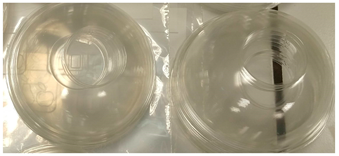 | Polylactic acid |
| 2 | Vegetable packaging (net) | 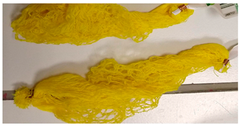 | Wood fibre |
| Source of Contaminated Samples | Contaminant Weight (g) | Total Sample Weight (g) | % Contamination |
|---|---|---|---|
| Packaging waste | 4.770 | 26.094 | 18% |
| Biowaste | 16.593 | 82.703 | 20% |
| Residual waste | 4.243 | 20.271 | 21% |
Disclaimer/Publisher’s Note: The statements, opinions and data contained in all publications are solely those of the individual author(s) and contributor(s) and not of MDPI and/or the editor(s). MDPI and/or the editor(s) disclaim responsibility for any injury to people or property resulting from any ideas, methods, instructions or products referred to in the content. |
© 2024 by the authors. Licensee MDPI, Basel, Switzerland. This article is an open access article distributed under the terms and conditions of the Creative Commons Attribution (CC BY) license (https://creativecommons.org/licenses/by/4.0/).
Share and Cite
Mhaddolkar, N.; Koinig, G.; Vollprecht, D.; Astrup, T.F.; Tischberger-Aldrian, A. Effect of Surface Contamination on Near-Infrared Spectra of Biodegradable Plastics. Polymers 2024, 16, 2343. https://doi.org/10.3390/polym16162343
Mhaddolkar N, Koinig G, Vollprecht D, Astrup TF, Tischberger-Aldrian A. Effect of Surface Contamination on Near-Infrared Spectra of Biodegradable Plastics. Polymers. 2024; 16(16):2343. https://doi.org/10.3390/polym16162343
Chicago/Turabian StyleMhaddolkar, Namrata, Gerald Koinig, Daniel Vollprecht, Thomas Fruergaard Astrup, and Alexia Tischberger-Aldrian. 2024. "Effect of Surface Contamination on Near-Infrared Spectra of Biodegradable Plastics" Polymers 16, no. 16: 2343. https://doi.org/10.3390/polym16162343
APA StyleMhaddolkar, N., Koinig, G., Vollprecht, D., Astrup, T. F., & Tischberger-Aldrian, A. (2024). Effect of Surface Contamination on Near-Infrared Spectra of Biodegradable Plastics. Polymers, 16(16), 2343. https://doi.org/10.3390/polym16162343