
Study on the Impact of Microscopic Pore Structure Characteristics in Tight Sandstone on Microscopic Remaining Oil after Polymer Flooding
 , and
, and
Abstract
:1. Introduction
2. Network Construction and Performance Parameters
2.1. Construction of the Digital Pore Network Model
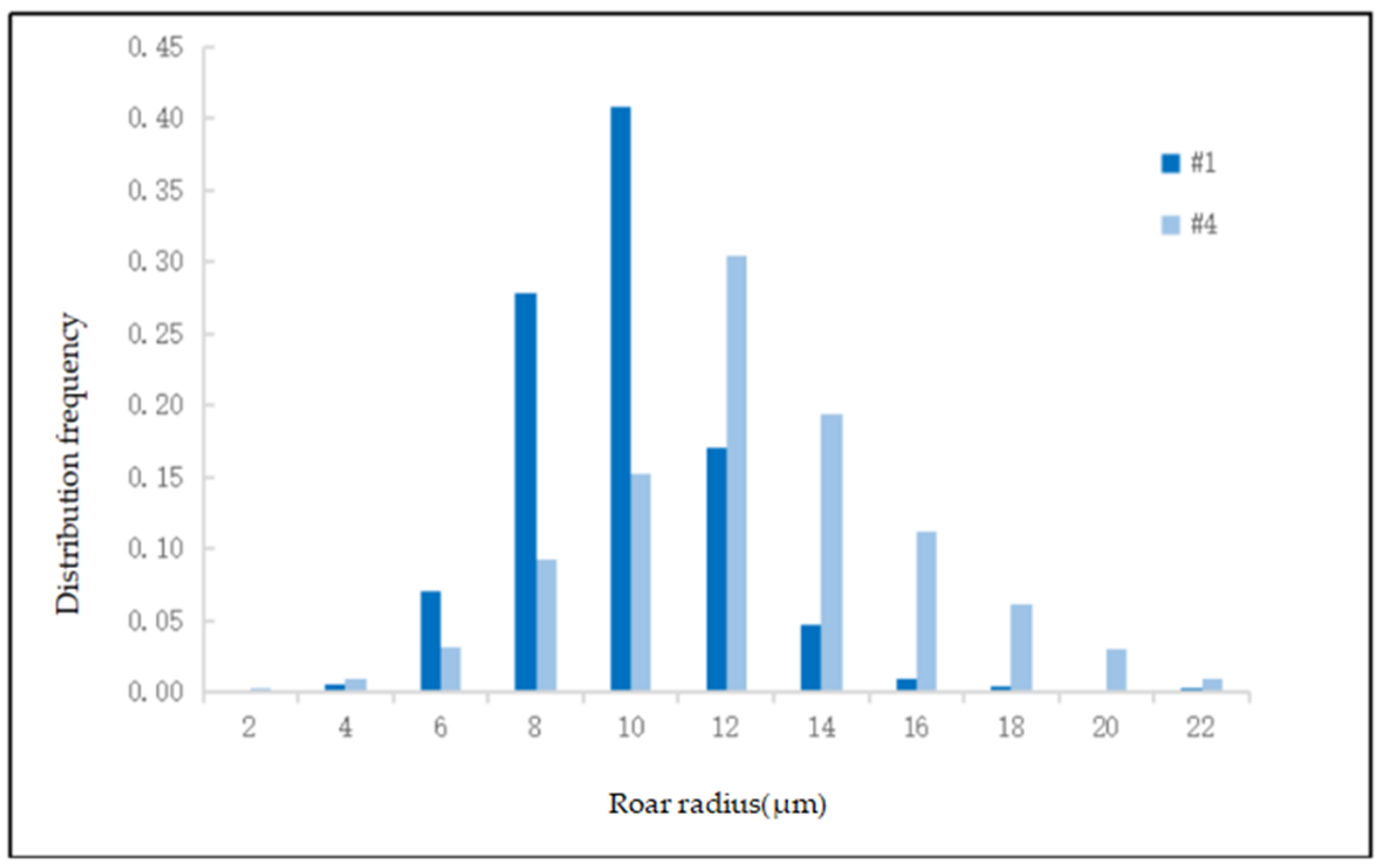
2.1.1. Pore Distribution Characteristics
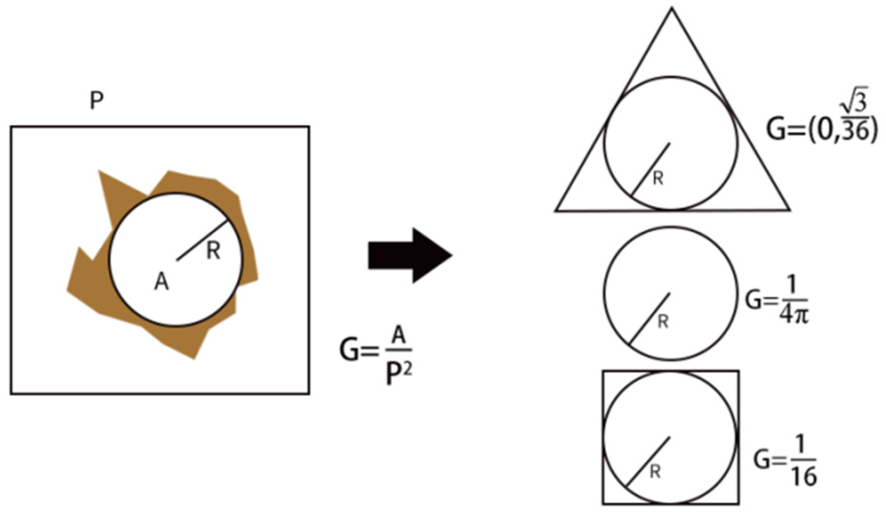
2.1.2. Geometric Characteristics of Pore–Throat Spaces
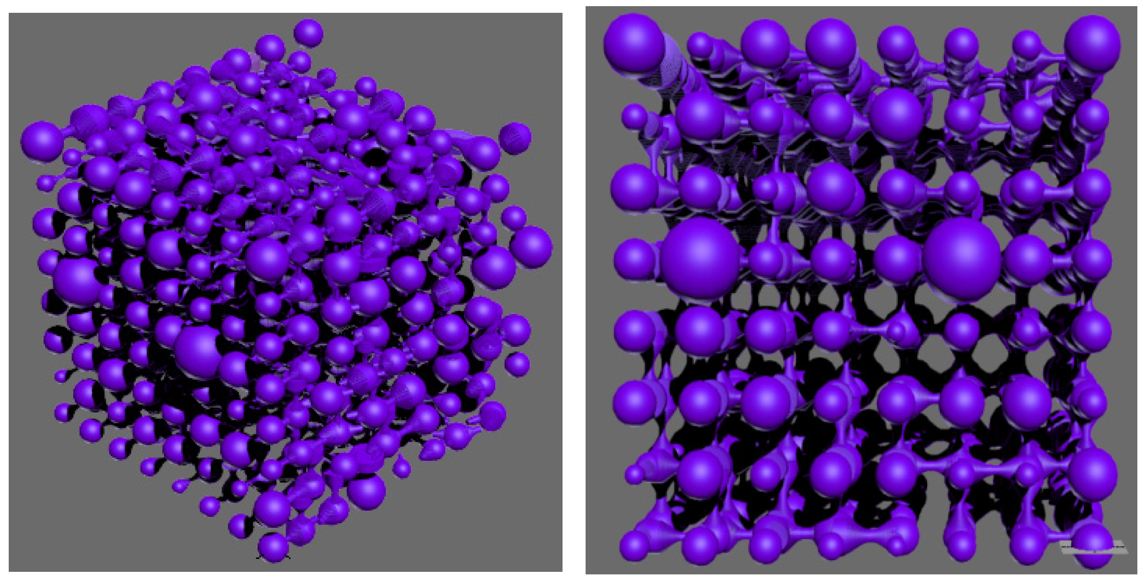
2.1.3. Construction and Visualization of the Pore–Throat Network Model
2.2. Performance Parameters
2.2.1. Calculation of Oil Saturation
2.2.2. Performance Parameters of Polymer Solution Systems
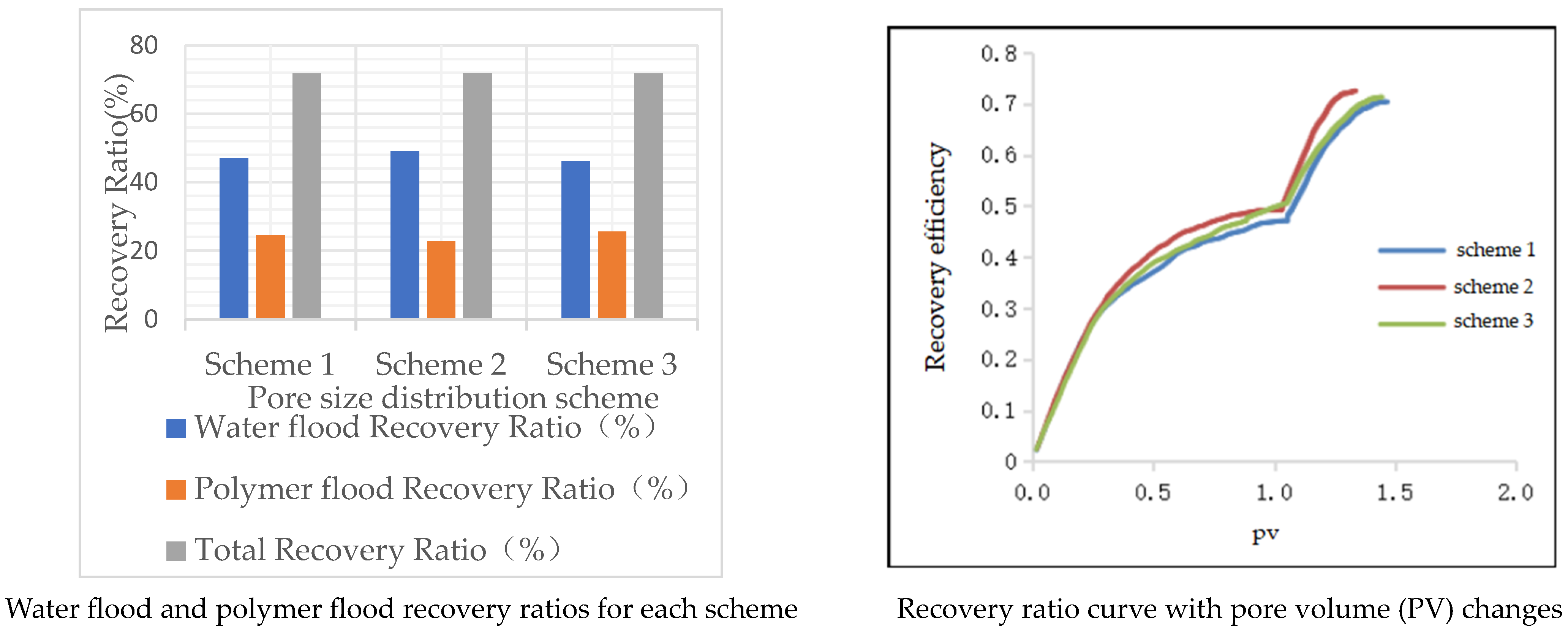
2.3. Experimental Data Validation
- Experimental Design: Select core samples with different pore structures to conduct polymer flooding experiments, measuring the oil recovery performance and residual oil distribution.
- 2.
- Data Analysis: Compare the experimental results with the simulation results to assess the credibility of the simulation outcomes. The specific experimental results are shown in Table 3.
- 3.
- Data Analysis: List the range of errors between the experimental and simulation results, analyze the sources of these errors, and improve the model accordingly.
- 4.
- Experimental Summary
3. The Impact of Pore Size Distribution on Various Types of Remaining Oil
3.1. The Impact of Pore Size Distribution on Oil Displacement Efficiency
3.2. Study on Residual Oil Distribution and Its Regularity When Pore Size Distribution Is Different
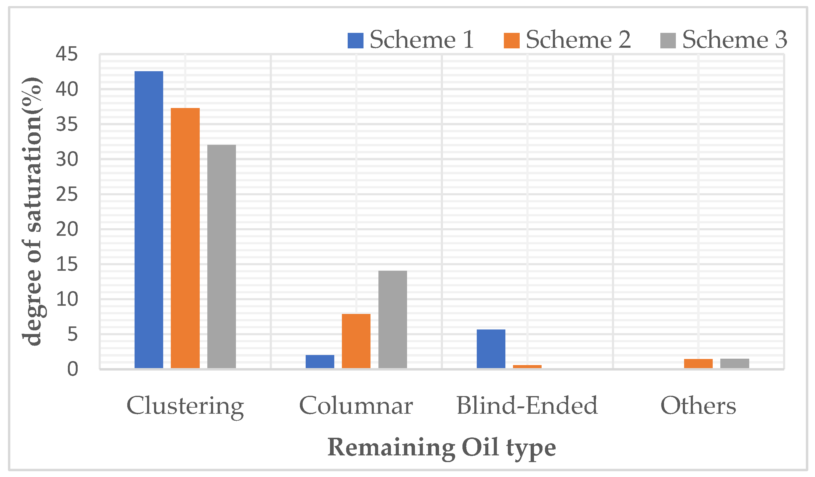
3.3. Study on Types and Quantitative Analysis of Residual Oil When Pore Size Distribution Is Different
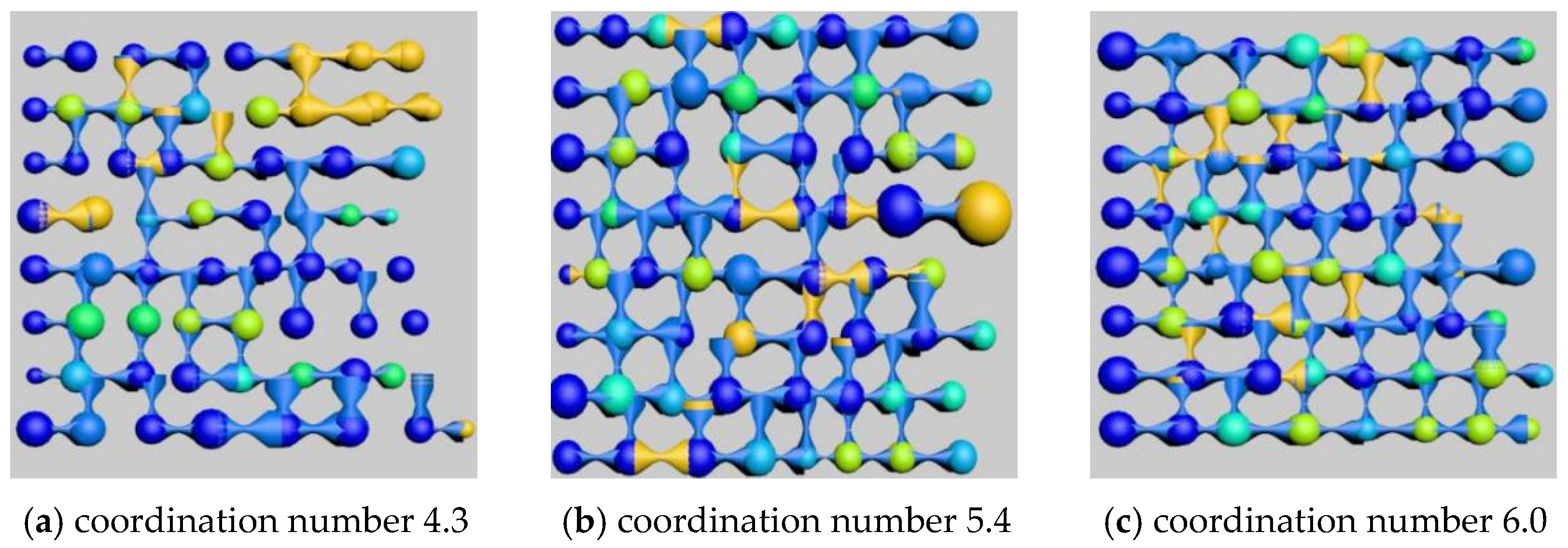
4. The Impact of Coordination Number on Various Types of Remaining Oil
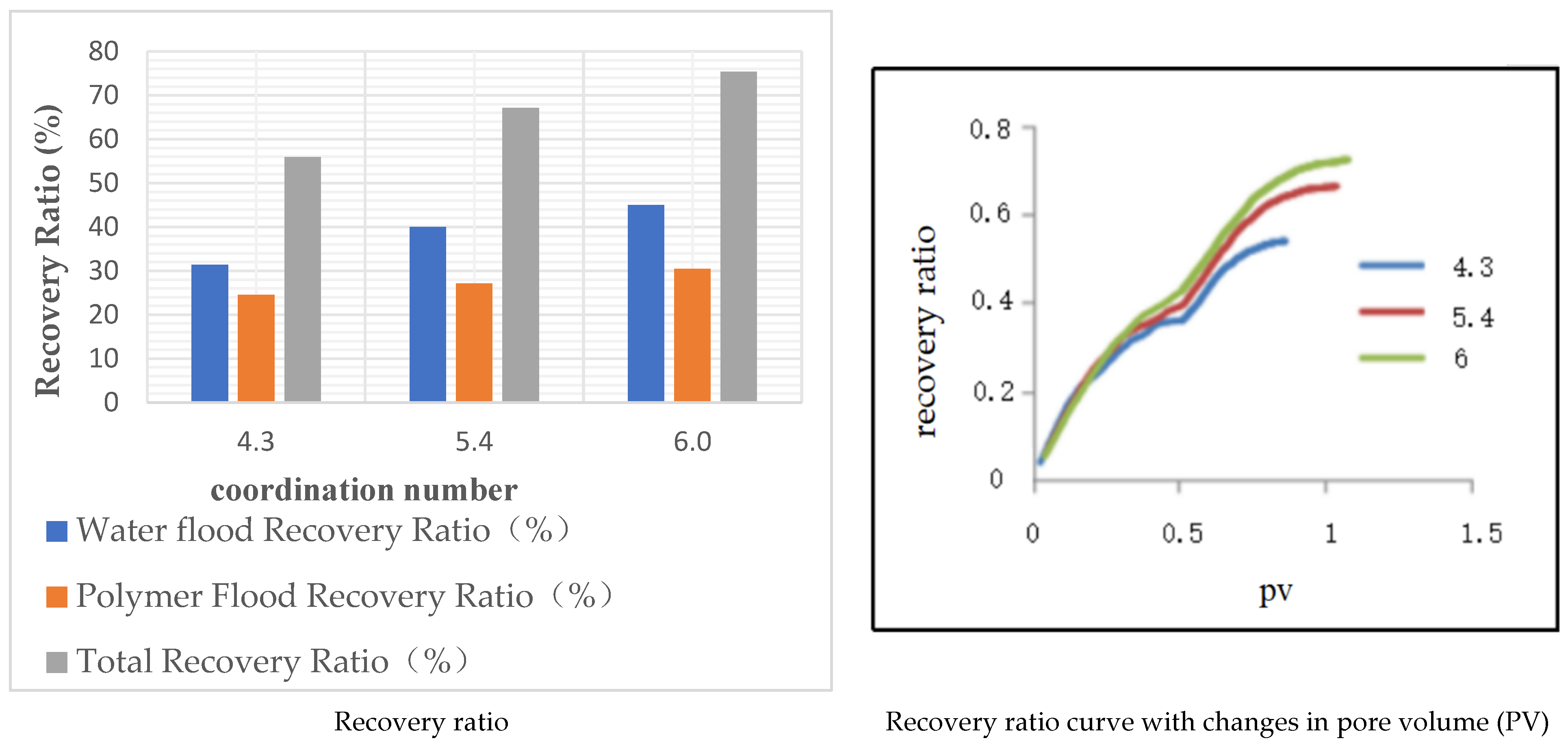
4.1. The Impact of Coordination Number on Various Types of Remaining Oil
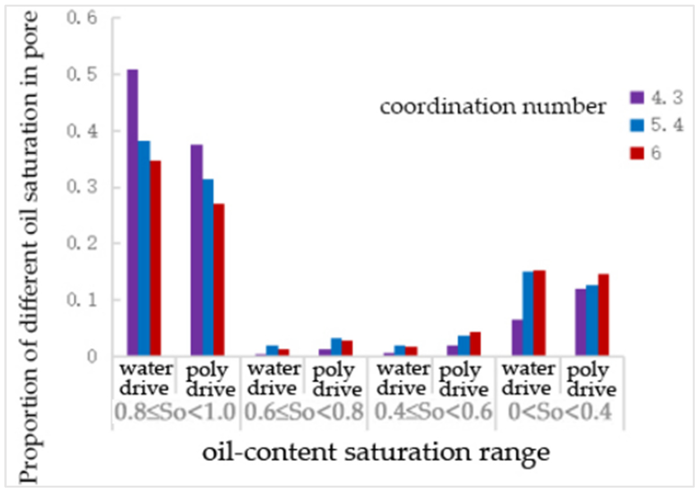
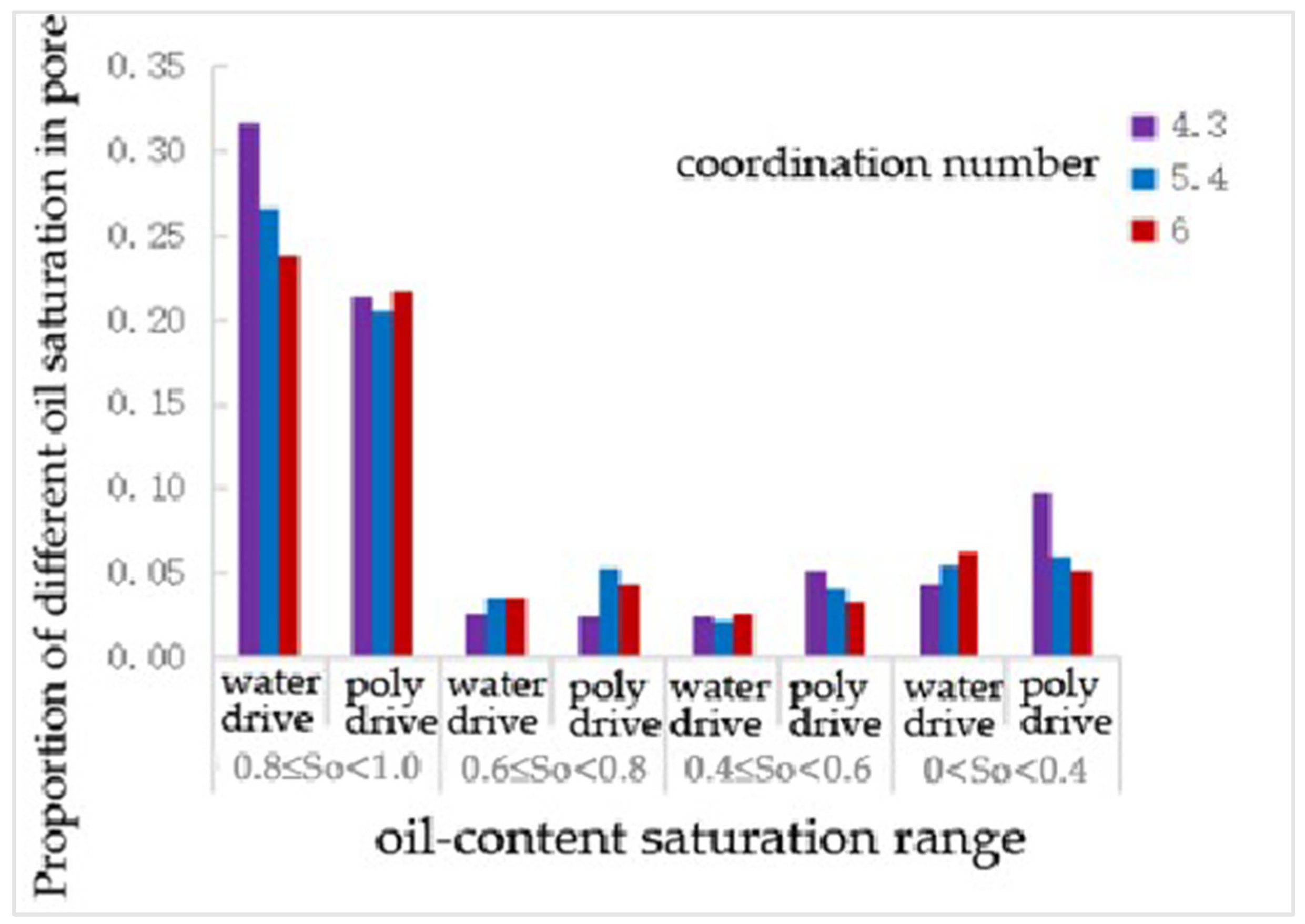
4.2. Study on Residual Oil Distribution and Its Regularity with Different Coordination Numbers
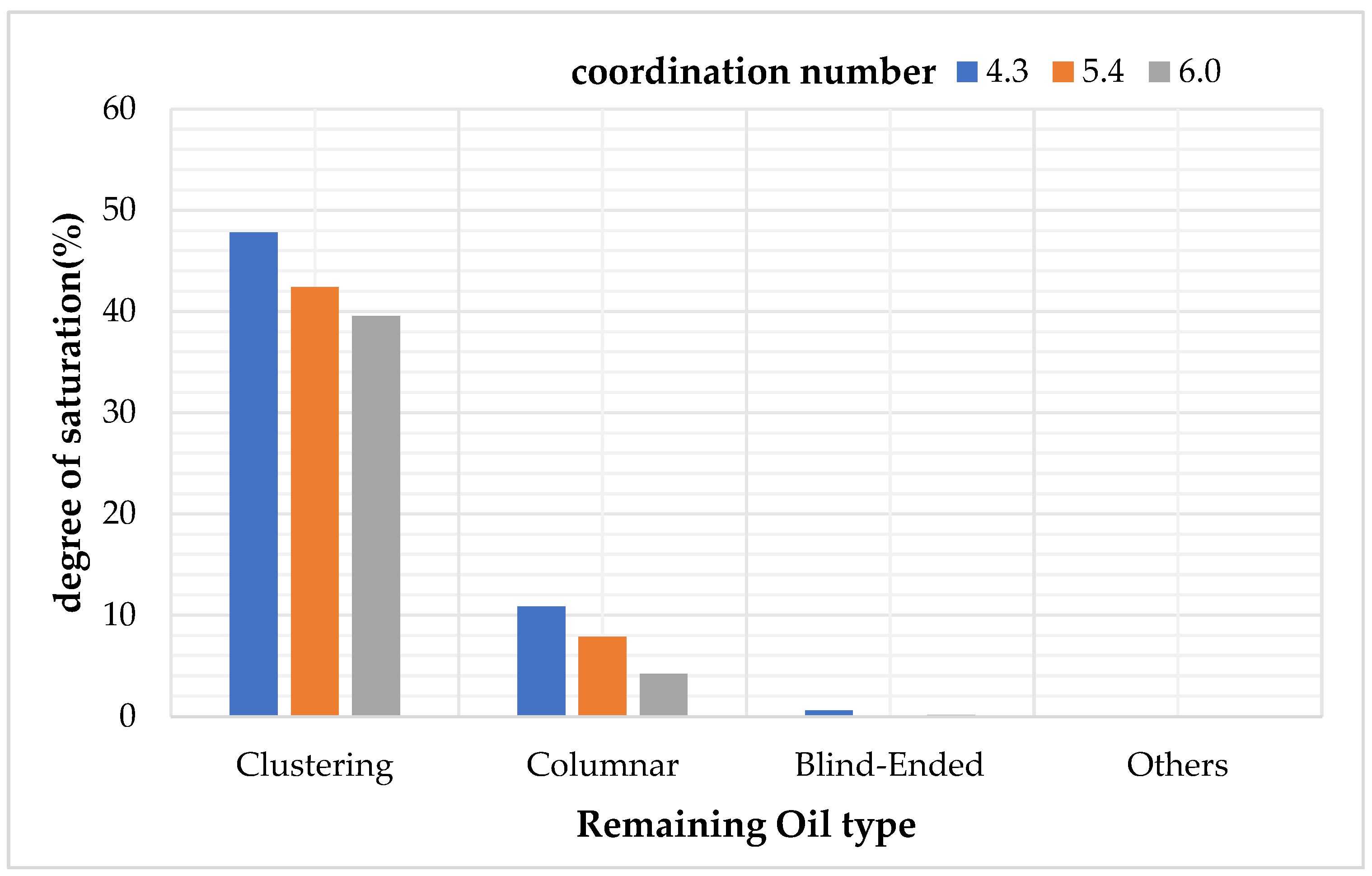
4.3. Study on Types and Quantitative Analysis of Residual Oil with Different Coordination Numbers
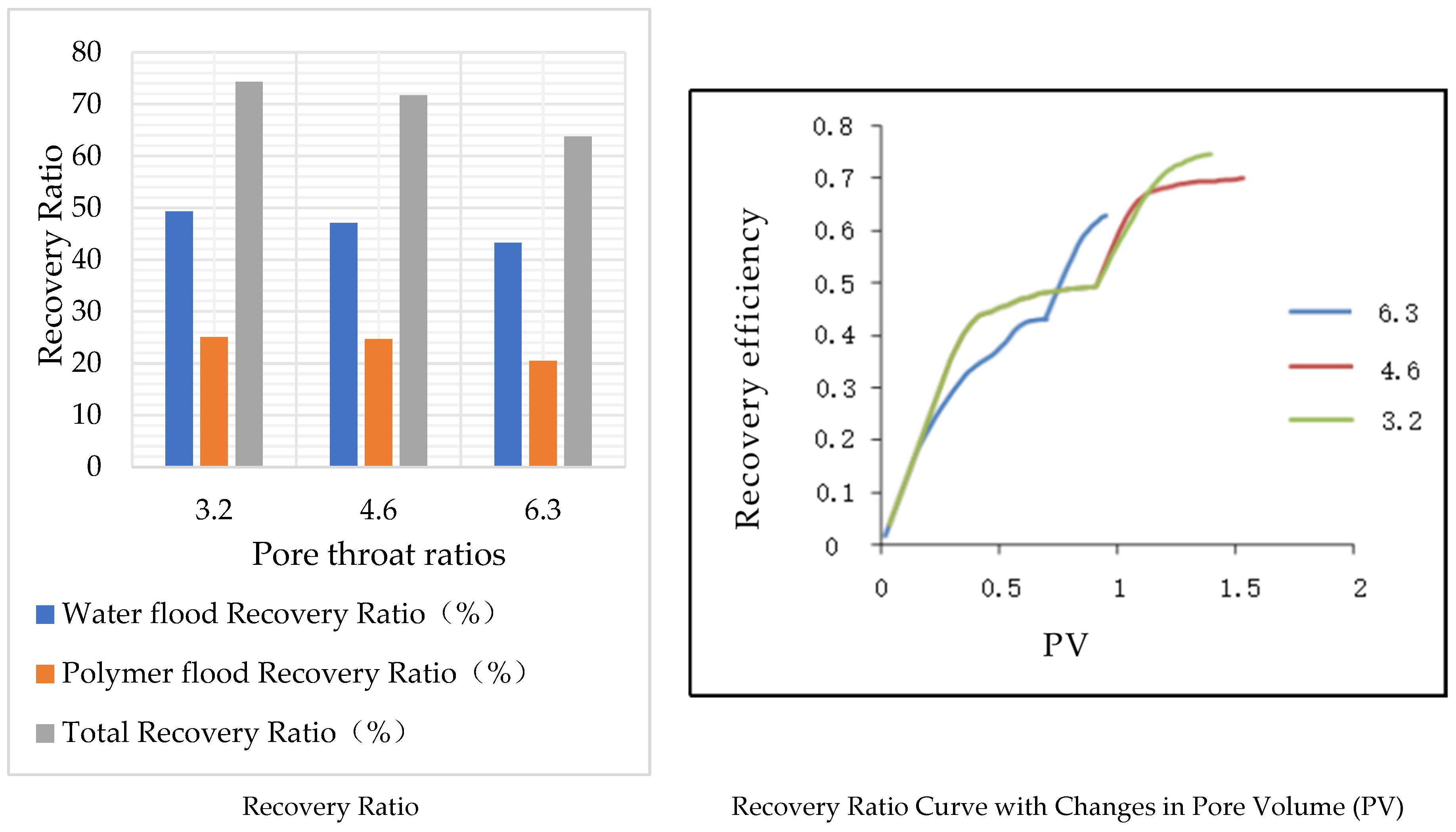
5. The Impact of Pore–Throat Ratio on Various Types of Remaining Oil
5.1. The Impact of Pore–Throat Ratio on Oil Displacement Efficiency
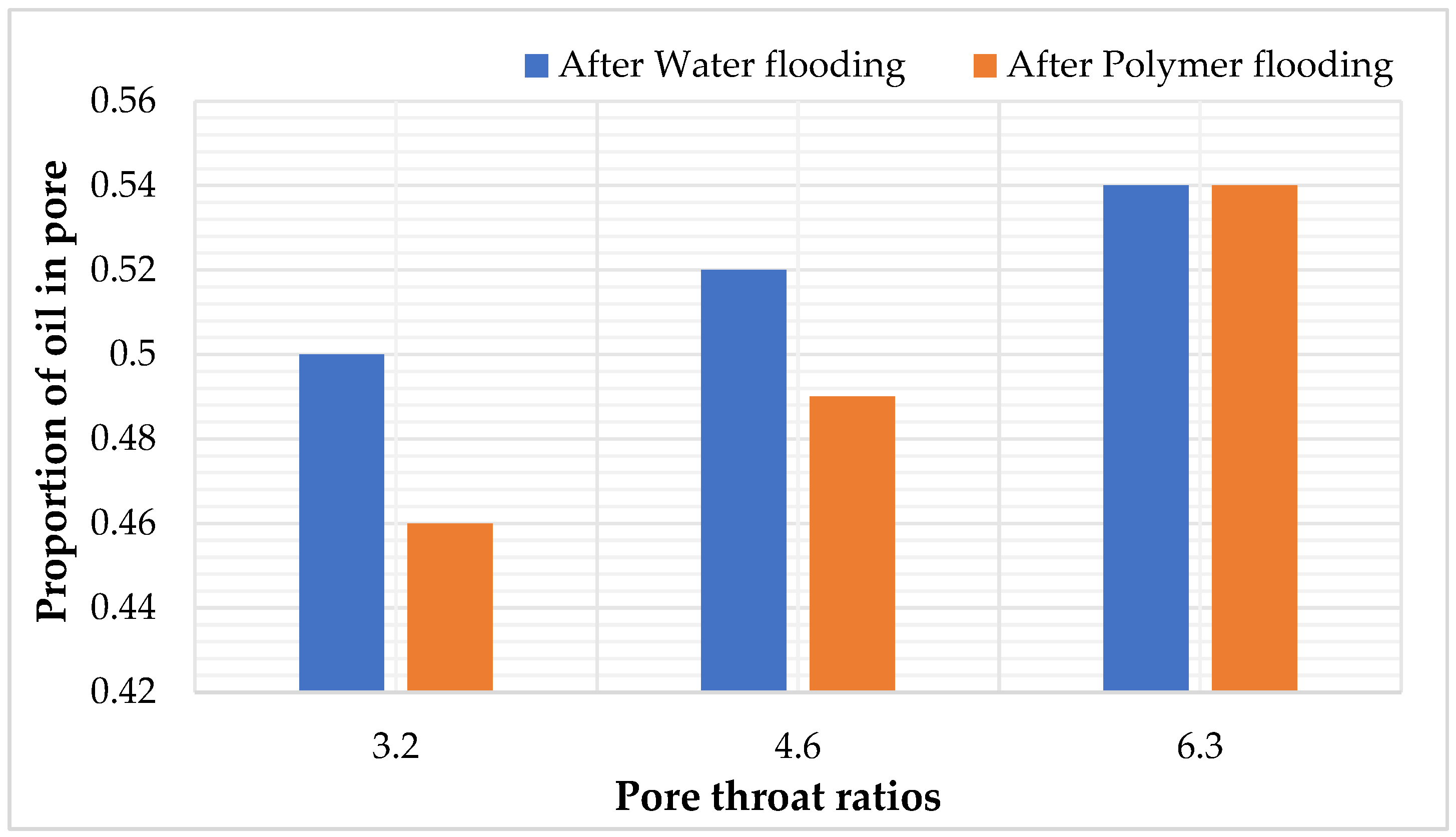
5.2. Study on Residual Oil Distribution and Its Regularity with Different Pore–Throat Ratios
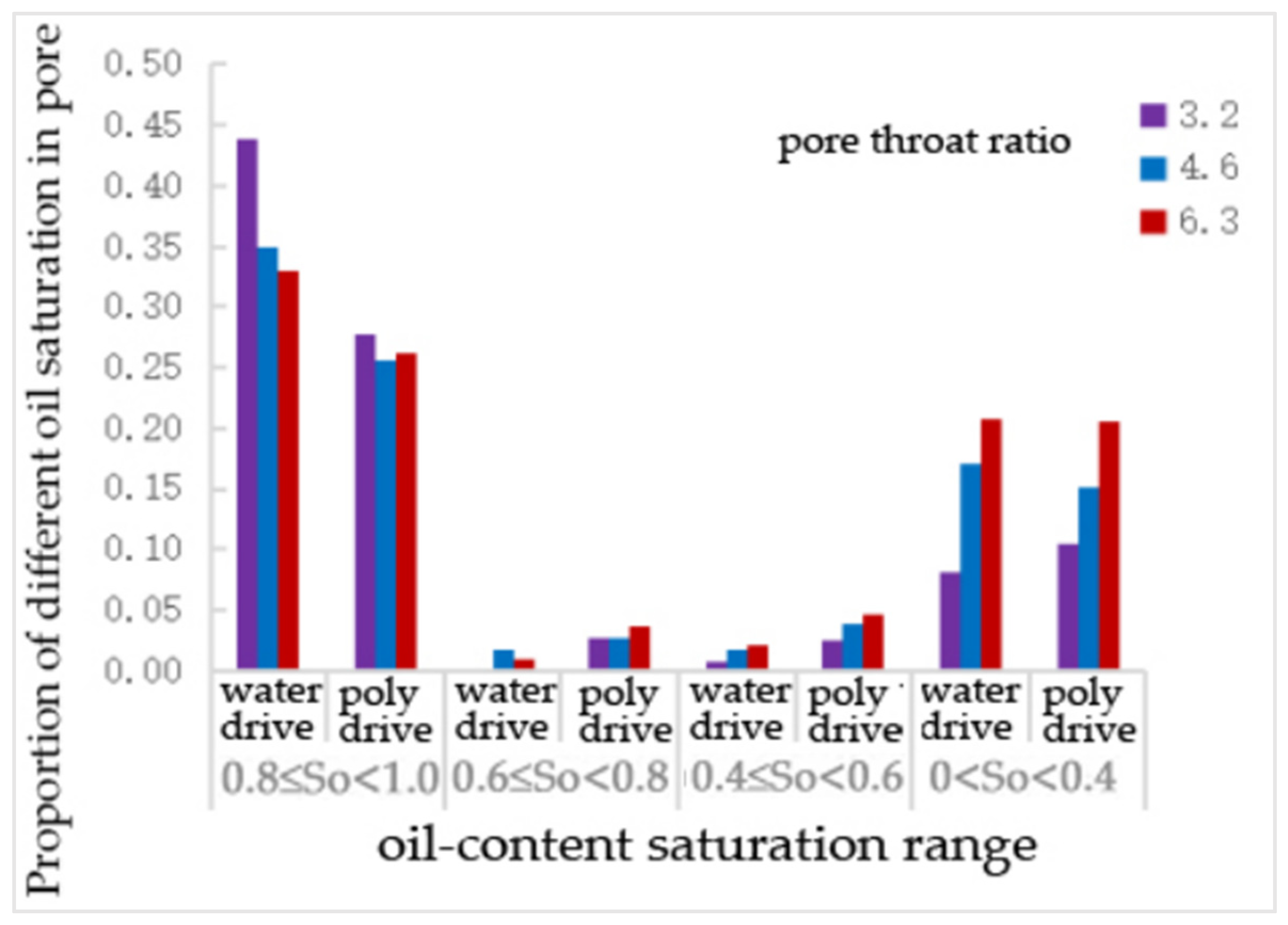
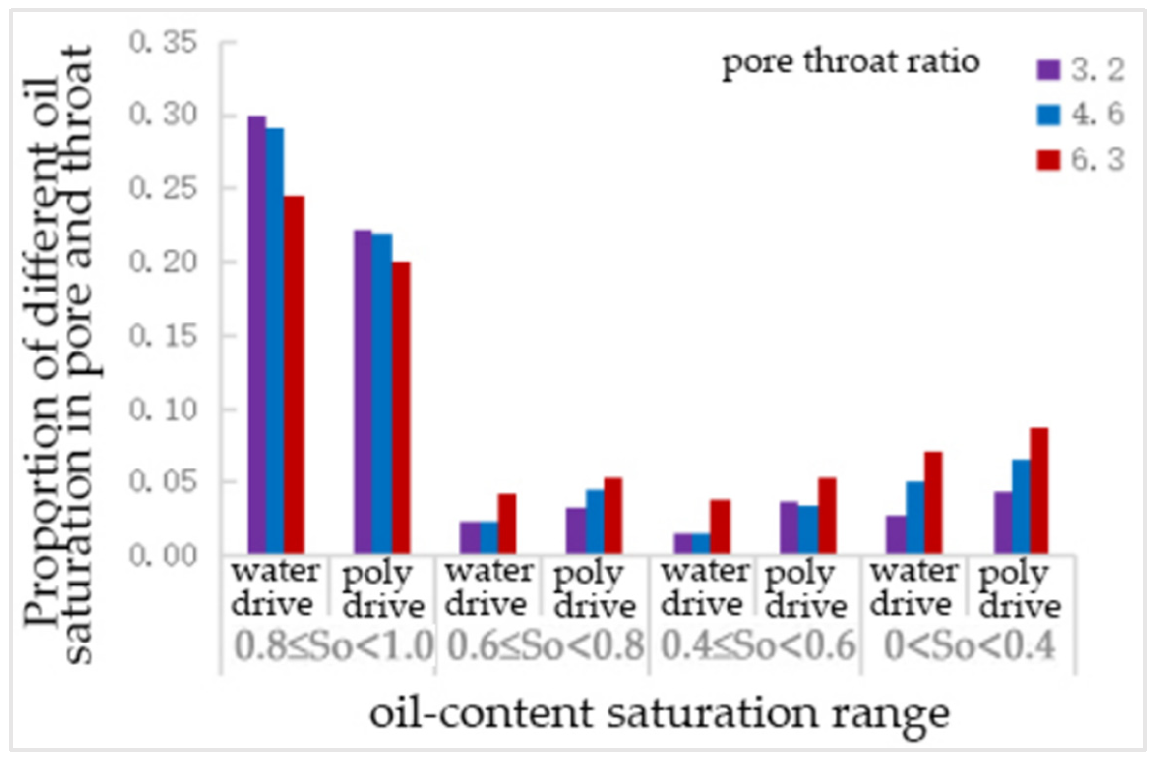
5.3. Study on Types and Quantitative Analysis of Residual Oil with Different Pore–Throat Ratios
6. The Impact of Wettability on Various Types of Remaining Oil
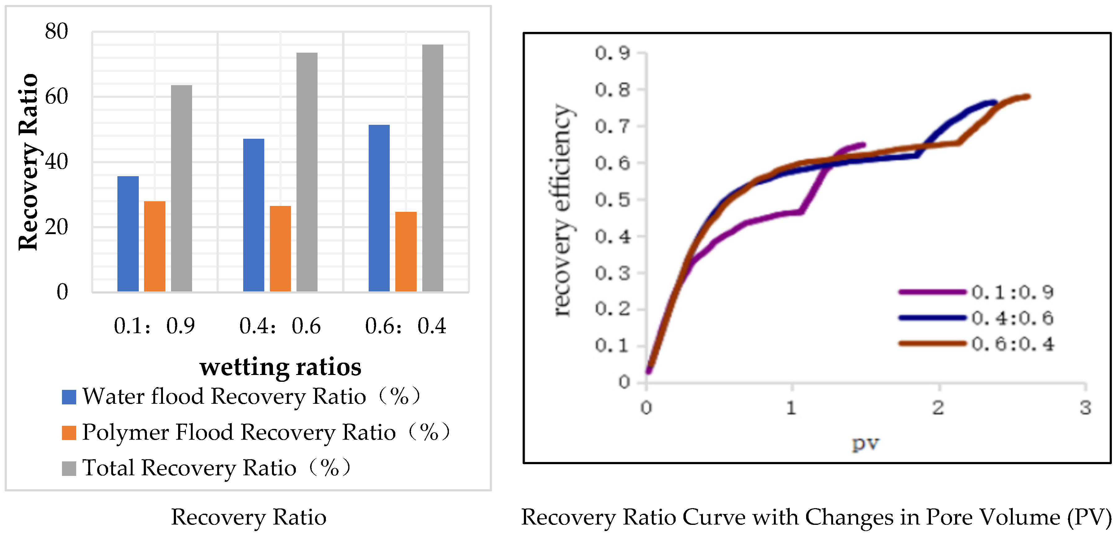
6.1. The Impact of Different Wettability Ratios on Oil Displacement Efficiency
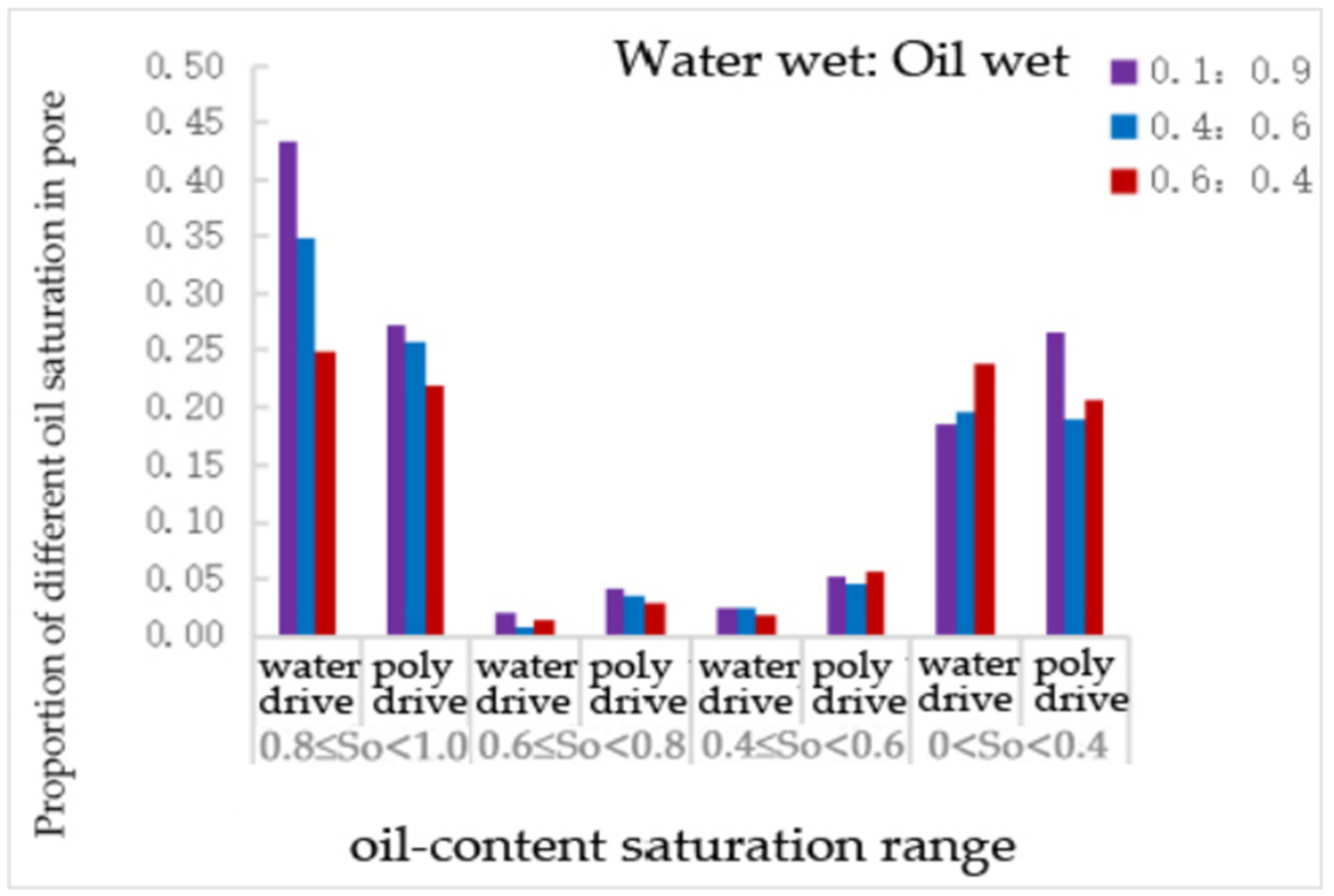
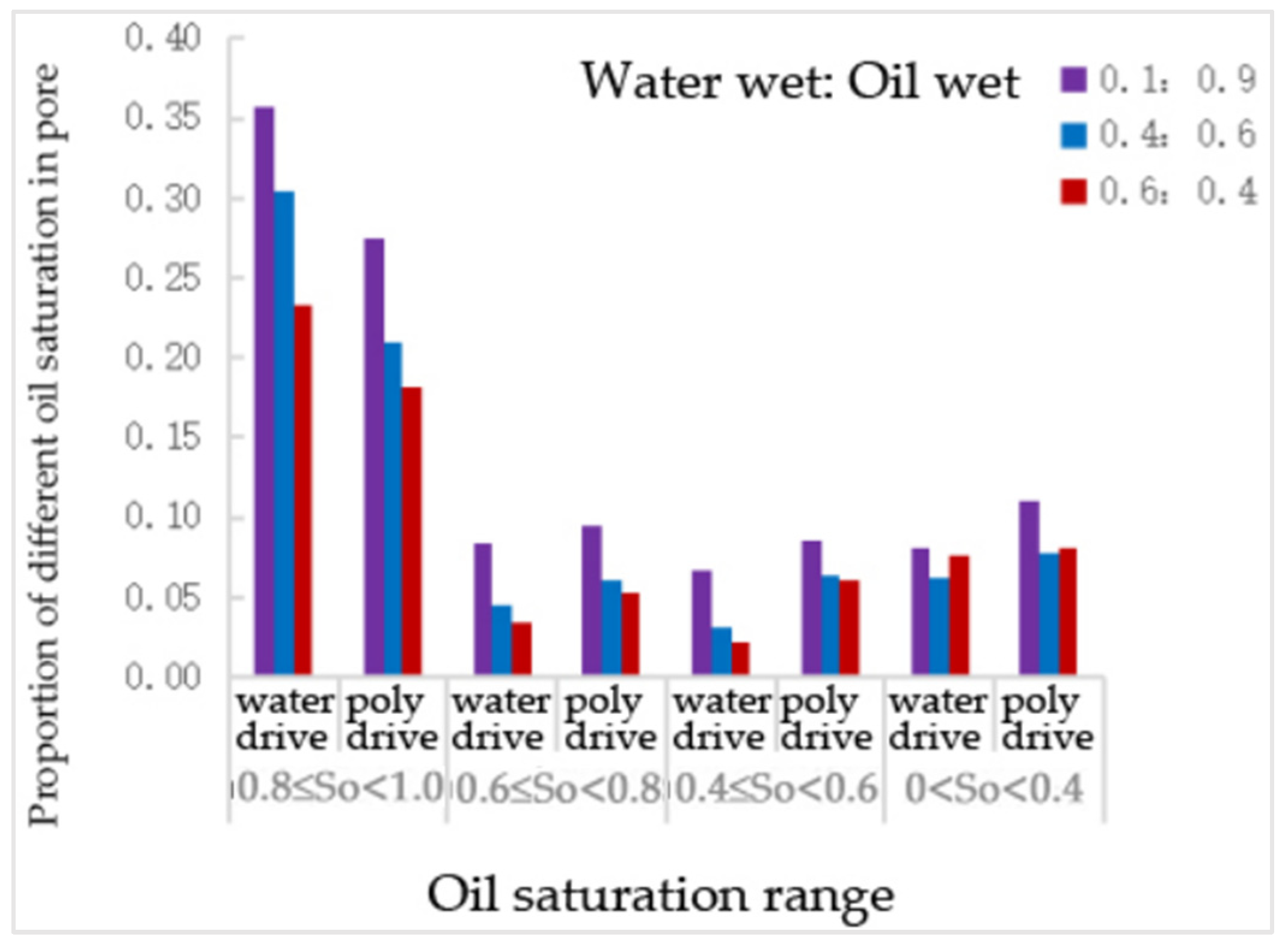
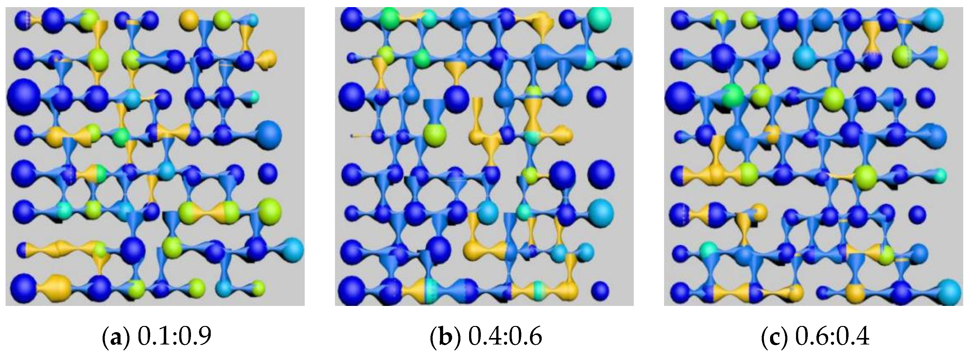
6.2. Study on Residual Oil Distribution and Its Regularity When Wettability Ratio Is Different
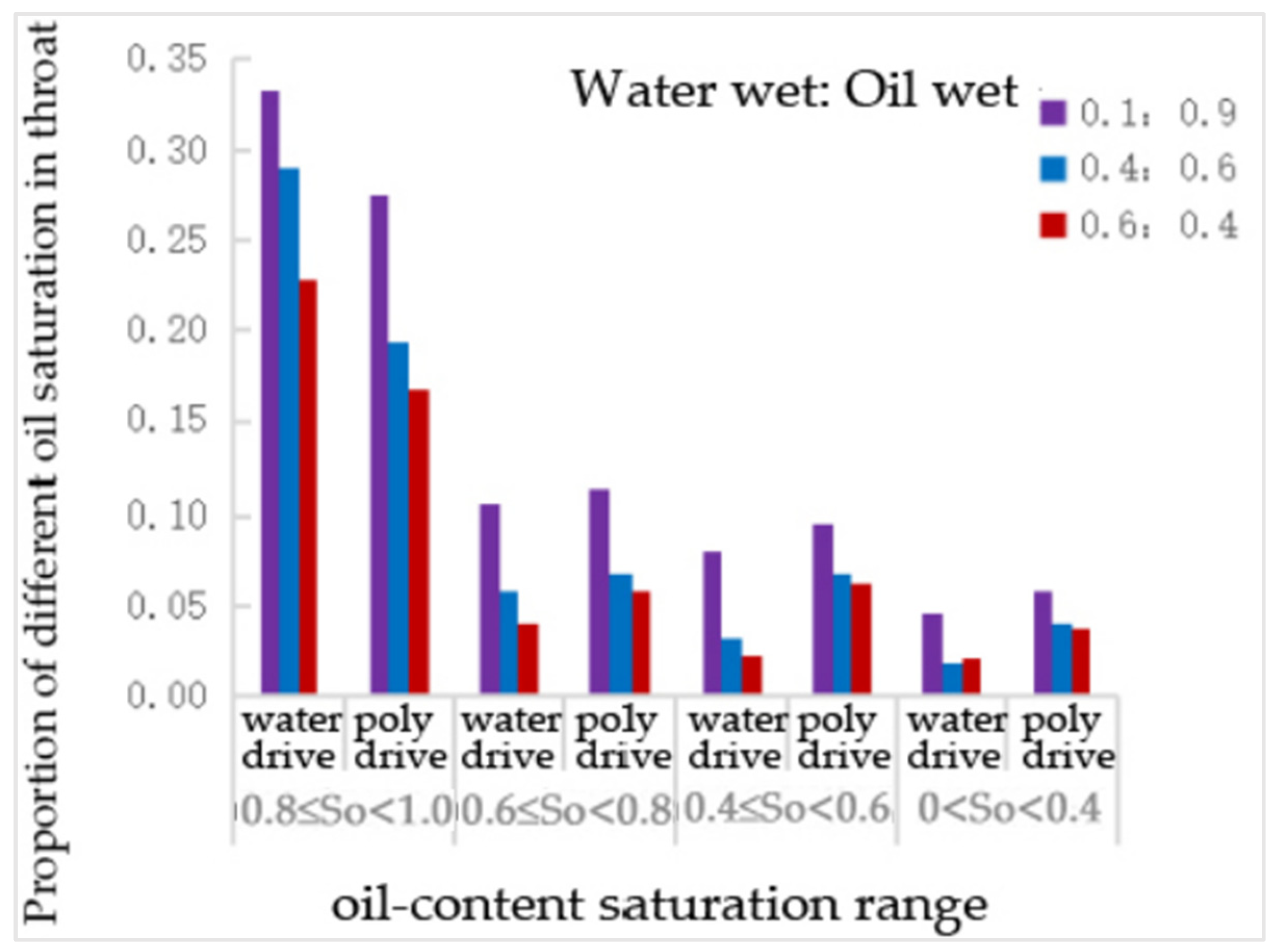
6.3. Study on Types and Quantitative Analysis of Residual Oil When Wettability Ratio Is Different
7. Conclusions
Author Contributions
Funding
Institutional Review Board Statement
Data Availability Statement
Conflicts of Interest
References
- Wang, Y.; Wu, Y.; Men, X. Stable production situation, challenges and prospects of old oil fields in China. Pet. Sci. Technol. Forum 2024, 43, 18–23+39. [Google Scholar]
- Ren, Z. Analysis on the current situation and difficulties of oil and natural gas development technology in China. China Pet. Chem. Ind. Stand. Qual. 2024, 44, 141–143. [Google Scholar]
- Wang, D. Research on “three yuan”, “two yuan” and “one yuan” oil flooding in Daqing Oilfield. Pet. Geol. Dev. Daqing 2003, 22, 1–9. [Google Scholar]
- Wang, P.; Liu, F.; Ma, F.; Yang, M.; Lin, Y.; Lu, C. Definition and distribution characteristics of the upper property limit of tight sandstone gas reservoir. Pet. Gas Geol. 2014, 35, 238–243. [Google Scholar]
- Zhang, C.; Zhu, D.; Luo, Q.; Liu, L.; Liu, D.; Yan, L.; Zhang, Y. Major factors controlling fracture development in the Middle Permian Lucaogou Formation tight oil reservoir, Junggar Basin, NW China. J. Asian Earth Sci. 2017, 146, 279–295. [Google Scholar] [CrossRef]
- Zhang, C.; Liu, D.-D.; Jiang, Z.-X.; Song, Y.; Luo, Q.; Wang, X. Mechanism for the formation of natural fractures and their effects on shale oil accumulation in Junggar Basin, NW China. Int. J. Coal Geol. 2022, 254, 103973. [Google Scholar] [CrossRef]
- Lowry, M.I.; Miller, C.T. Pore-Scale Modeling of Nonwetting-Phase Residual in Porous Media. Water Resour. Res. 1995, 31, 455–474. [Google Scholar] [CrossRef]
- Mohammadi, S.; Sorbie, K.S.; Danesh, A.; Peden, J.M. Pore-level modeling of gas-condensate flow through horizontal porous media. In Proceedings of the SPE Annual Technical Conference and Exhibition, New Orleans, LA, USA, 23–26 September 1990. SPE 20479. [Google Scholar]
- Zhao, Z. Study on the distribution law of residual oil in three class oil layers of Lambei East Block. Contemp. Chem. Ind. 2015, 44, 773–774+796. [Google Scholar]
- Bai, Z.; Wang, Q.; Li, Y. Distribution law of microscopic residual oil in polymer flooding in sandstone oilfield. Daqing Pet. Geol. Dev. 2021, 40, 101–106. [Google Scholar]
- Friedman, S.R.; Zhang, L.; Seaton, N.A. Gas and solute diffusion coefficients in pore networks and its description by a simple capillary model. Transp. Porous Media 1995, 19, 281–301. [Google Scholar] [CrossRef]
- Dixit, A.B.; Mcdougall, S.R.; Soosbie, K.S. Pore-scale modeling of wettability effects and their influence on oil recovery. SPE Reserv. Eval. Eng. 1999, 2, 25–36. [Google Scholar] [CrossRef]
- Akin, S.; Erzeybek, S. Pore network modeling of two phase flow in vuggy carbonates. In Proceedings of the SPE Europec Featured at EAGE Conference and Exhibition, Rome, Italy, 9–12 June 2008. SPE 113884. [Google Scholar]
- Raoof, A.; Majid Hassanizadeh, S. A new method for generating pore-network models of porous media. Transp. Porous Media 2010, 81, 391–407. [Google Scholar] [CrossRef]
- Yang, Z.; Cheng, T.; Luo, T.; Li, J.; Yan, W.; Hou, J. Method of microscopic residual oil distribution and EOR evaluation. Oilfield Chem. 2024, 41, 356–366. [Google Scholar]
- Wang, C.; Han, S.; Du, H.; Yang, Y.; Sun, X.; Dong, Y.; Liu, J.; Bian, X. Unogeneity characteristics of low permeability lithologic reservoir and distribution law of water flooding residual oil in Dongying Depression. Front. Mar. Geol. 2024, 40, 36–43. [Google Scholar]
- Wang, M. Study on Residual Oil Distribution in Ultra-Low Permeability Reservoir and Encryption of Short Horizontal Wells. Master’s Thesis, Xi’an Petroleum University, Xi’an, China, 2023. [Google Scholar]
- Cyganek, B. Color image segmentation with support vector machines: Applications to road signs detection. Int. J. Neural Syst. 2008, 18, 339–345. [Google Scholar] [CrossRef] [PubMed]
- Kumar Pandey, R.; Gandomkar, A.; Vaferi, B.; Kumar, A.; Torabi, F. Supervised deep learning-based paradigm to screen the enhanced oil recovery scenarios. Sci. Rep. 2023, 13, 4892. [Google Scholar] [CrossRef]
- Krizhevsky, A.; Sutskever, I.; Hinton, G.E. Imagenet classification with deep convolutional neural networks. In Proceedings of the 26th Annual Conference on Neural Information Processing Systems 2012, Lake Tahoe, NV, USA, 3–6 December 2012; pp. 1097–1105. [Google Scholar]
- Qiao, Y.; Song, D.; Liu, W.; Yu, Z. Study on pore structure characteristics and evolution of coal Formation shale in the eastern margin of Ordos Basin. J. Henan Polytech. Univ. (Nat. Sci. Ed.) 2024, 43, 53–66. [Google Scholar]
- Hu, X.; Yao, W.; Hu, Z.; Huang, F.; Wang, Y.; Wang, X. Pore structure characterization and development master factors of deep coal rock reservoir in Xishan Kiln Formation in Baijiahai Region of Junggar Basin. J. China Univ. Pet. (Nat. Sci. Ed.) 2024, 48, 12–23. [Google Scholar]
- Tang, H.; Liu, X.; Chen, Y.; Yu, W.; Zhao, N.; Shi, X.; Wang, M.; Liao, J. Differences in shale pore structure of different tectonic units and their geological significance of oil and gas—Take deep shale in Luzhou region, Sichuan Basin as an example. Nat. Gas Ind. 2024, 44, 16–28. [Google Scholar]
- Deng, J.; Dong, W.; Socher, R.; Li, L.; Li, K.; Li, F. Imagenet: A large-scale hierarchical image database. In Proceedings of the 2009 IEEE Conference on Computer Vision and Pattern Recognition, Miami, FL, USA, 20–25 June 2009; pp. 248–255. [Google Scholar]
- Long, J.; Shelhamer, E.; Darrell, T. Fully convolutional networks for semantic segmentation. In Proceedings of the IEEE Conference on Computer Vision and Pattern Recognition, Boston, MA, USA, 7–12 June 2015; pp. 3431–3439. [Google Scholar]
- Liang-Chieh, C.; Papandreou, G.; Kokkinos, I.; Murphy, K.; Yuille, A. Semantic image segmentation with deep convolutional nets and fully connected crfs. In Proceedings of the International Conference on Learning Representations (ICLR), San Diego, CA, USA, 7–9 May 2015. [Google Scholar]
- Li, X. Study of Rock Pore Structure and Simulation Based on Three-Dimensional Digital Core. Master’s Thesis, China University of Geosciences, Wuhan, China, 2021. [Google Scholar]
- Wang, Z.; Cong, S.; Chen, W.; Han, Y.; Yang, H. Matmatching relationship between the hydrodynamic size and the reservoir throat size of the binary drive system. Oilfield Chem. 2024, 41, 296–301. [Google Scholar]
- Li, J. Study on the Evolution Characteristics of Dispersed Cohesive Soil Cracks in Qian’an Region. Master’s Thesis, Jilin University, Changchun, China, 2024. [Google Scholar] [CrossRef]
- Xu, S.; Zhang, J.; Shi, X. Characterization of stratigraphic factors and pore ratio in sandstone strata. Logging Tech. 2023, 47, 146–151. [Google Scholar]
- Zhang, J.; Zhang, S.; Gao, W.; Hu, S.; Wang, Z. A fractal model of the thermal diffusion coefficient in the porous media. Appl. Math. Mech. 2022, 43, 553–560. [Google Scholar]
- Chen, X. Method of calculating the relative permeability of dense sandstone reservoir with introduced hole-throat ratio. Liaoning Chem. Ind. 2022, 51, 104–107. [Google Scholar]
- Liu, H.; Xu, Y.; Wang, C.; Ding, F.; Xiao, H. Study on the linkages between microstructure and permeability of porous media using pore network and BP neural network. Mater. Res. Express 2022, 9, 025504. [Google Scholar] [CrossRef]
- Yang, Q.-H.; Guo, D.; Li, M.-Y.; Dai, L.-Y.; Haidenbauer, J.; Meißner, U.-G. Study of the electromagnetic form factors of the nucleons in the timelike region. J. High Energy Phys. 2024, 2024, 208. [Google Scholar] [CrossRef]
- Qiao, H. Effect of Microscopic Pore Structure Parameters on the Efficiency of Polymer Flooding. Master’s Thesis, Northeastern Petroleum University, Daqing, China, 2015. [Google Scholar]
- Howard, A.G.; Zhu, M.; Chen, B.; Kalenichenko, D.; Wang, W.; Weyand, T.; Andreetto, M.; Adam, H. MobileNets: Efficient convolutional neural networks for mobile vision applications. arXiv 2017, arXiv:1704.04861. [Google Scholar]
- Cao, G.; Lin, M.; Zhang, L.; Ji, L.; Jiang, W. Numerical simulation of the dynamic mechanism of oil transport and oil saturation prediction in dense sandstone. Sci. China Earth Sci. 2024, 54, 186–202. [Google Scholar]
- Guo, T.; Zhang, J.; Chai, J.; Bao, B.; Sun, J. Method of calculating shale oil saturation to gas-oil ratio based on logging data. Pet. Drill. Technol. 2023, 51, 126–136. [Google Scholar]
- Zhang, R. Study on the Microscopic Flow Characteristics of Viscoelastic Polymer Flooding Ordinary Thick Oil. Master’s Thesis, Northeastern Petroleum University, Daqing, China, 2023. [Google Scholar]
- Yan, R. Movement Characteristics of the Polymer Used for Flooding in the Reservoir Pore. Master’s Thesis, China University of Petroleum, Beijing, China, 2022. [Google Scholar]
- Zhou, F. Evaluation of Surface Active Polymer Performance and Flooding Efficiency. Master’s Thesis, Northeastern Petroleum University, Daqing, China, 2018. [Google Scholar]
- Wang, X. Practices and benefit evaluation of enhanced oil recovery in binary compound flooding reservoirs. Petrochem. Technol. 2024, 31, 162–164. [Google Scholar]
- Tian, T.; Jia, J.; Shi, S.; Zhang, H.; Huang, T.; Shi, Z. Study on the viscosity-temperature characteristics of lubricating oil considering shear rate and gas holdup. Lubr. Eng. 2024, 49, 160–167. [Google Scholar]
- Alghazwani, Y.; Talath, S.; Fatima, F.; Ghazwani, M.; Alamri, A.H.; Hani, U.; Osmani, R.A. Investigating the thermal enhancement of Levetiracetam solubility in the ternary system of supercritical carbon dioxide and ethanol. J. Mol. Liq. 2024, 411, 125692. [Google Scholar] [CrossRef]


| Core Number Model Parameter | #1 | #2 | #3 | #4 | #5 |
|---|---|---|---|---|---|
| Porosity (%) | 25.1 | 24.6 | 24.1 | 26.3 | 27.6 |
| Water measurement permeability (10−3 μm2) | 370 | 39 | 430 | 568 | 623 |
| Length of the larynx (μm) | 21~187 | 3~65 | 8~155 | 15~167 | 16~168 |
| Throat radius (μm) | 1~20 | 1~16 | 1~18 | 1~22 | 1~25 |
| Mean coordination number | 4.2 | 4.3 | 4.6 | 4.1 | 4.2 |
| Average pore–throat ratio | 5.4 | 5.1 | 4.7 | 4.3 | 4.2 |
| Throat Radius (μm) | 2 | 4 | 6 | 8 | 10 | 12 | 14 | 16 | 18 | 20 | 22 |
|---|---|---|---|---|---|---|---|---|---|---|---|
| #1 distribution frequency | 0.002 | 0.005 | 0.071 | 0.279 | 0.409 | 0.17 | 0.047 | 0.01 | 0.004 | 0.002 | 0.001 |
| #4 distribution frequency | 0.001 | 0.010 | 0.031 | 0.092 | 0.153 | 0.305 | 0.194 | 0.112 | 0.062 | 0.030 | 0.010 |
| Experiment | Digital Model | Physical Model | Digital Model | Physical Model | Digital Model | Physical Model |
|---|---|---|---|---|---|---|
| Core number porosity (%) | #1 25.6 | #3 31.77 | #4 27.25 | |||
| Permeability (10−3 μm2) | 370 | 430 | 568 | |||
| Water drive recovery rate (%) | 45.03 | 47.07 | 46.56 | 49.12 | 44.17 | 46.22 |
| Poly drive recovery rate (%) | 23.69 | 24.65 | 21.49 | 22.76 | 23.68 | 25.58 |
| Total recovery rate (%) | 68.72 | 71.71 | 68.05 | 71.88 | 67.85 | 71.76 |
| Scheme | 1 | 2 | 3 |
|---|---|---|---|
| Core ID Porosity (%) | #1 25.6 | #3 31.77 | #4 27.25 |
| Permeability ( μm2) | 370 | 430 | 568 |
| Water flood recovery ratio (%) | 47.07 | 49.12 | 46.22 |
| Polymer flood recovery ratio (%) | 24.65 | 22.76 | 25.58 |
| Total recovery ratio (%) | 71.71 | 71.88 | 71.76 |
| Pore Distribution Scheme | Scheme 1 | Scheme 2 | Scheme 3 | |
|---|---|---|---|---|
| Total throat count | Total throat count | 993 | 993 | 993 |
| Total pore count | 512 | 512 | 512 | |
| After water flooding | Number of oil-bearing throats | 510 | 480 | 508 |
| Number of oil-bearing pores | 280 | 273 | 284 | |
| Total number of oil-bearing entities | 790 | 753 | 792 | |
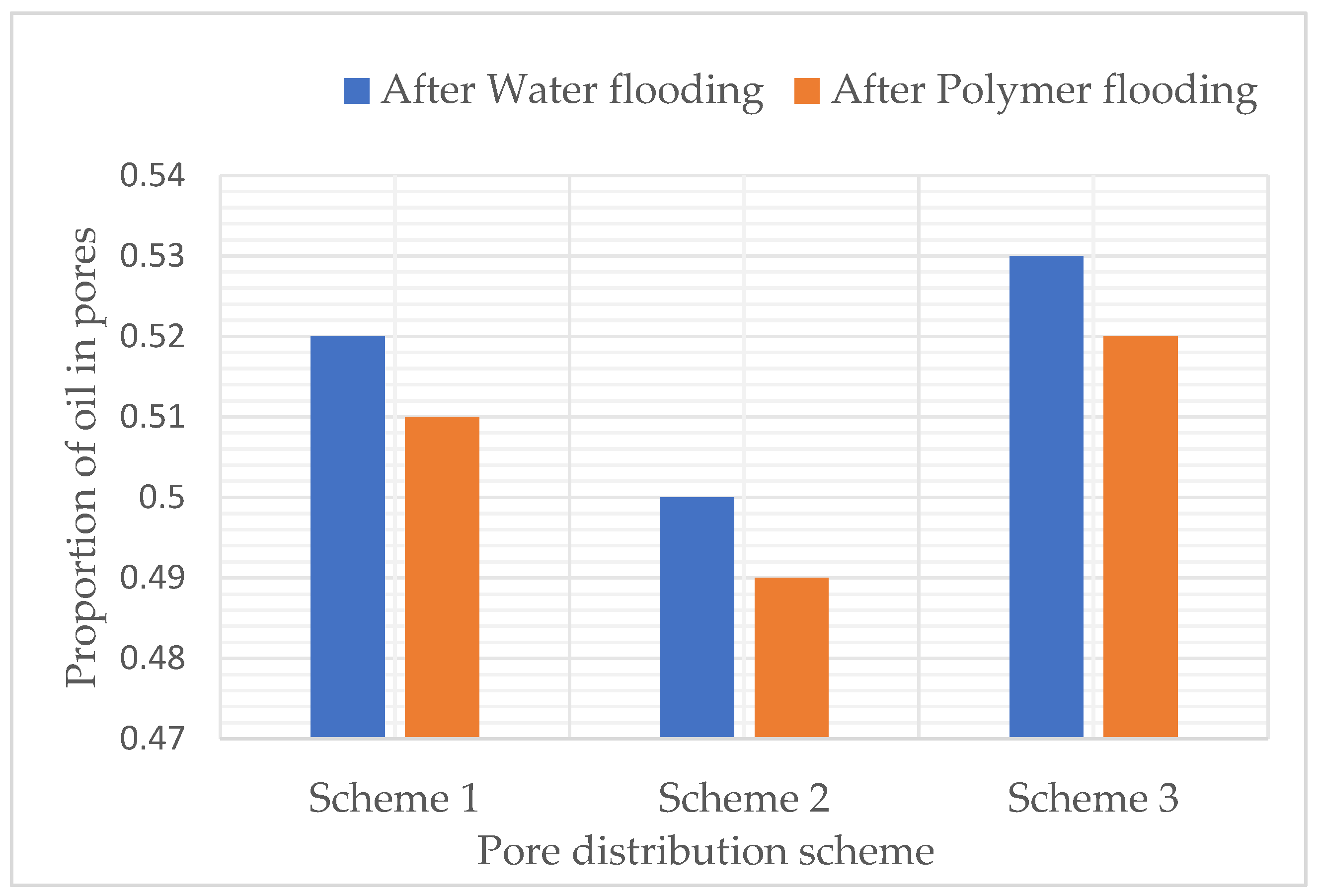
| Oil saturation in pores | 0.52 | 0.50 | 0.53 | |
| After polymer flooding | Number of oil-bearing throats | 486 | 472 | 496 |
| Number of oil-bearing pore | 275 | 261 | 283 | |
| Total number of oil-bearing entities | 761 | 733 | 779 | |
| Oil saturation in pores | 0.51 | 0.49 | 0.52 | |
| Oil Saturation | 0.8 ≤ So < 1 | 0.6 ≤ So < 0.8 | 0.4 ≤ So < 0.6 | 0 < So < 0.4 | 0 | |||||
|---|---|---|---|---|---|---|---|---|---|---|
| Ratio Scheme | Water Flooding | Polymer Flooding | Water Flooding | Polymer Flooding | Water Flooding | Polymer Flooding | Water Flooding | Polymer Flooding | Water Flooding | Polymer Flooding |
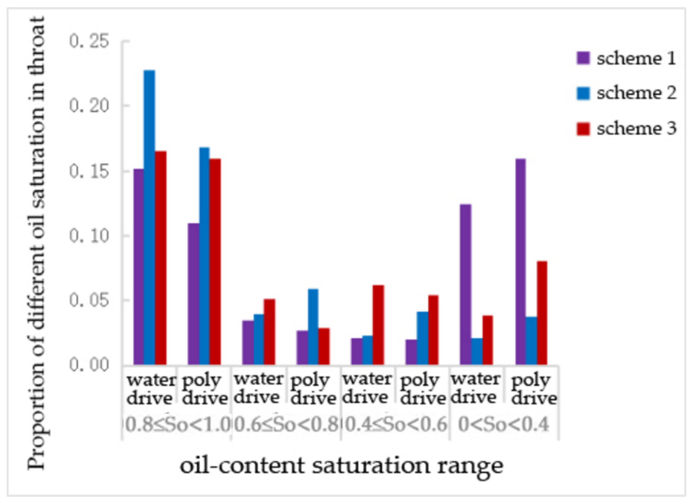
| Scheme 1 | 0.152 | 0.110 | 0.035 | 0.027 | 0.021 | 0.020 | 0.124 | 0.159 | 0.668 | 0.684 |
| Scheme 2 | 0.228 | 0.168 | 0.040 | 0.059 | 0.023 | 0.042 | 0.021 | 0.038 | 0.688 | 0.693 |
| Scheme 3 | 0.165 | 0.159 | 0.051 | 0.029 | 0.062 | 0.054 | 0.039 | 0.081 | 0.669 | 0.677 |
| Oil Saturation | 0.8 ≤ So < 1 | 0.6 ≤ So < 0.8 | 0.4 ≤ So < 0.6 | 0 < So < 0.4 | 0 | |||||
|---|---|---|---|---|---|---|---|---|---|---|
| Ratio Scheme | Water Flooding | Polymer Flooding | Water Flooding | Polymer Flooding | Water Flooding | Polymer Flooding | Water Flooding | Polymer Flooding | Water Flooding | Polymer Flooding |
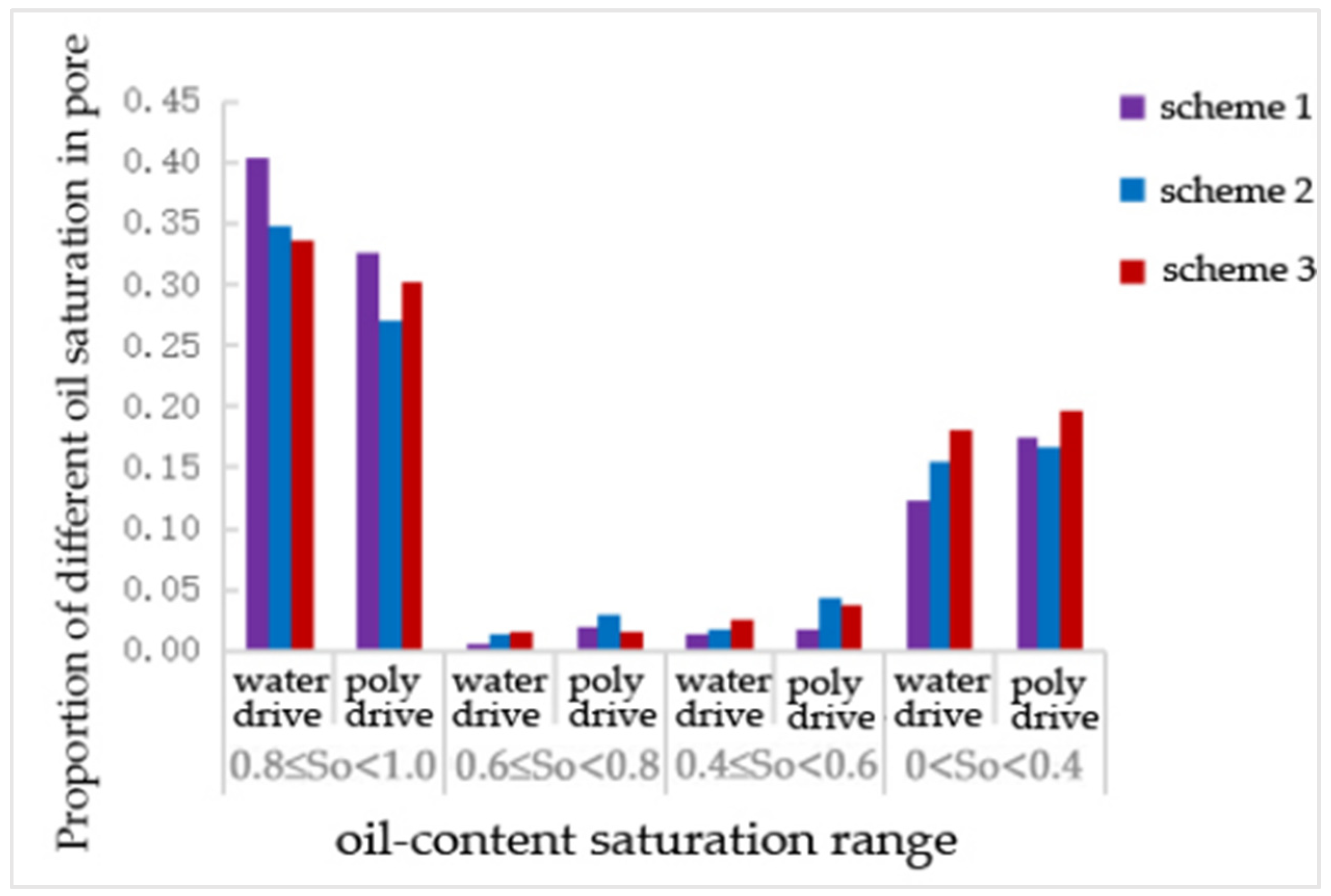
| Scheme 1 | 0.404 | 0.326 | 0.006 | 0.020 | 0.014 | 0.018 | 0.123 | 0.174 | 0.453 | 0.463 |
| Scheme 2 | 0.348 | 0.271 | 0.014 | 0.029 | 0.018 | 0.043 | 0.154 | 0.166 | 0.467 | 0.490 |
| Scheme 3 | 0.336 | 0.303 | 0.016 | 0.016 | 0.025 | 0.037 | 0.180 | 0.197 | 0.445 | 0.447 |
| Type | Saturation (%) | ||
|---|---|---|---|
| Scheme 1 | Scheme 2 | Scheme 3 | |
| Clustering | 42.52 | 37.29 | 32.05 |
| Columnar | 1.99 | 7.88 | 14.04 |
| Blind-ended | 5.67 | 0.56 | 0.01 |
| Others | 0.03 | 1.43 | 1.49 |
| Coordination Number | 4.3 | 5.4 | 6.0 |
|---|---|---|---|
| Porosity (%) | 25.59 | 25.86 | 25.52 |
| Permeability (10−3 μm2) | 243.62 | 375.36 | 483.59 |
| Water flood recovery ratio (%) | 31.35 | 39.99 | 44.98 |
| Polymer flood recovery ratio (%) | 24.57 | 27.13 | 30.44 |
| Total recovery ratio (%) | 55.92 | 67.12 | 75.42 |
| Coordination Number | 4.3 | 5.4 | 6.0 | |
|---|---|---|---|---|
| Total throat count | Total throat count | 822 | 1016 | 1120 |
| Total pore count | 512 | 512 | 512 | |
| After water flooding | Number of oil-bearing throats | 541 | 480 | 469 |
| Number of oil-bearing pores | 299 | 292 | 273 | |
| Total number of oil-bearing entities | 840 | 772 | 742 | |
| Oil saturation in throats | 0.63 | 0.51 | 0.45 | |
| After polymer flooding | Number of oil-bearing throats | 519 | 472 | 455 |
| Number of oil-bearing pores | 272 | 262 | 251 | |
| Total number of oil-bearing entities | 791 | 734 | 706 | |
| Oil saturation in throats | 0.59 | 0.48 | 0.43 | |
| Oil Saturation | 0.8 ≤ So < 1 | 0.6 ≤ So < 0.8 | 0.4 ≤ So < 0.6 | 0 < So < 0.4 | 0 | |||||
|---|---|---|---|---|---|---|---|---|---|---|
| Ratio Coordination Number | Water Flooding | Polymer Flooding | Water Flooding | Polymer Flooding | Water Flooding | Polymer Flooding | Water Flooding | Polymer Flooding | Water Flooding | Polymer Flooding |
| 4.3 | 0.253 | 0.159 | 0.034 | 0.029 | 0.030 | 0.061 | 0.035 | 0.090 | 0.648 | 0.662 |
| 5.4 | 0.228 | 0.168 | 0.040 | 0.059 | 0.023 | 0.042 | 0.021 | 0.038 | 0.688 | 0.693 |
| 6.0 | 0.201 | 0.199 | 0.042 | 0.048 | 0.029 | 0.029 | 0.033 | 0.020 | 0.695 | 0.704 |
| Oil Saturation | 0.8 ≤ So < 1 | 0.6 ≤ So < 0.8 | 0.4 ≤ So < 0.6 | 0 < So < 0.4 | 0 | |||||
|---|---|---|---|---|---|---|---|---|---|---|
| Ratio Coordination Number | Water Flooding | Polymer Flooding | Water Flooding | Polymer Flooding | Water Flooding | Polymer Flooding | Water Flooding | Polymer Flooding | Water Flooding | Polymer Flooding |
| 4.3 | 0.508 | 0.375 | 0.004 | 0.014 | 0.006 | 0.021 | 0.066 | 0.121 | 0.416 | 0.469 |
| 5.4 | 0.381 | 0.314 | 0.020 | 0.033 | 0.020 | 0.037 | 0.150 | 0.127 | 0.430 | 0.488 |
| 6.0 | 0.348 | 0.271 | 0.014 | 0.029 | 0.018 | 0.043 | 0.154 | 0.146 | 0.467 | 0.510 |
| Ratio Coordination Number | 0.8 ≤ So < 1 | 0.6 ≤ So < 0.8 | 0.4 ≤ So < 0.6 | 0 < So < 0.4 | 0 | |||||
|---|---|---|---|---|---|---|---|---|---|---|
| Ratio Coordination Number | Water Flooding | Polymer Flooding | Water Flooding | Polymer Flooding | Water Flooding | Polymer Flooding | Water Flooding | Polymer Flooding | Water Flooding | Polymer Flooding |
| 4.3 | 0.317 | 0.213 | 0.026 | 0.025 | 0.024 | 0.051 | 0.043 | 0.098 | 0.590 | 0.614 |
| 5.4 | 0.266 | 0.205 | 0.035 | 0.053 | 0.022 | 0.041 | 0.054 | 0.060 | 0.623 | 0.642 |
| 6.0 | 0.238 | 0.217 | 0.035 | 0.043 | 0.026 | 0.032 | 0.063 | 0.052 | 0.638 | 0.655 |
| Type | Saturation (%) | ||
|---|---|---|---|
| Coordination Number 4.3 | Coordination Number 5.4 | Coordination Number 6.0 | |
| Clustering | 47.79 | 42.41 | 39.55 |
| Columnar | 10.84 | 7.89 | 4.21 |
| Blind-ended | 0.61 | 0.01 | 0.15 |
| Other | 0.01 | 0.01 | 0.03 |
| Pore–Throat Ratio | 3.2 | 4.6 | 6.3 |
|---|---|---|---|
| Porosity (%) | 25.47 | 25.86 | 25.66 |
| Permeability (10−3 μm2) | 954.43 | 544.12 | 329.05 |
| Water flood recovery ratio (%) | 49.32 | 47.07 | 43.29 |
| Polymer flood recovery ratio (%) | 25.02 | 24.65 | 20.43 |
| Total recovery ratio (%) | 74.34 | 71.72 | 63.72 |
| Pore–Throat Ratio | 3.2 | 4.6 | 6.3 | |
|---|---|---|---|---|
| Total throat count | Total throat count | 993 | 993 | 993 |
| Total pore count | 512 | 512 | 512 | |
| After water flooding | Number of oil-bearing throats | 482 | 494 | 518 |
| Number of oil-bearing pores | 271 | 284 | 290 | |
| Total number of oil-bearing entities | 753 | 778 | 808 | |
| Oil saturation in throats | 0.50 | 0.52 | 0.54 | |
| After polymer flooding | Number of oil-bearing throats | 465 | 501 | 526 |
| Number of oil-bearing pores | 222 | 243 | 282 | |
| Total number of oil-bearing entities | 687 | 742 | 808 | |
| Oil saturation in throats | 0.46 | 0.49 | 0.54 | |
| Oil Saturation | 0.8 ≤ So < 1 | 0.6 ≤ So < 0.8 | 0.4 ≤ So < 0.6 | 0 < So < 0.4 | 0 | |||||
|---|---|---|---|---|---|---|---|---|---|---|
| Ratio of Pore–Throat Ratio | Water Flooding | Polymer Flooding | Water Flooding | Polymer Flooding | Water Flooding | Polymer Flooding | Water Flooding | Polymer Flooding | Water Flooding | Polymer Flooding |
| 3.2 | 0.255 | 0.203 | 0.031 | 0.035 | 0.019 | 0.041 | 0.010 | 0.024 | 0.686 | 0.697 |
| 4.6 | 0.271 | 0.207 | 0.025 | 0.051 | 0.015 | 0.032 | 0.010 | 0.036 | 0.678 | 0.674 |
| 6.3 | 0.216 | 0.179 | 0.052 | 0.060 | 0.044 | 0.055 | 0.025 | 0.049 | 0.663 | 0.658 |
| Oil Saturation | 0.8 ≤ So < 1 | 0.6 ≤ So < 0.8 | 0.4 ≤ So < 0.6 | 0 < So < 0.4 | 0 | |||||
|---|---|---|---|---|---|---|---|---|---|---|
| Ratio of Pore–Throat Ratio | Water Flooding | Polymer Flooding | Water Flooding | Polymer Flooding | Water Flooding | Polymer Flooding | Water Flooding | Polymer Flooding | Water Flooding | Polymer Flooding |
| 3.2 | 0.438 | 0.277 | 0.002 | 0.027 | 0.008 | 0.025 | 0.082 | 0.104 | 0.471 | 0.566 |
| 4.6 | 0.350 | 0.256 | 0.018 | 0.027 | 0.018 | 0.039 | 0.170 | 0.152 | 0.445 | 0.525 |
| 6.3 | 0.330 | 0.262 | 0.010 | 0.037 | 0.020 | 0.047 | 0.207 | 0.205 | 0.434 | 0.449 |
| Oil Saturation | 0.8 ≤ So < 1 | 0.6 ≤ So < 0.8 | 0.4 ≤ So < 0.6 | 0 < So < 0.4 | 0 | |||||
|---|---|---|---|---|---|---|---|---|---|---|
| Ratio of Pore–Throat Ratio | Water Flooding | Polymer Flooding | Water Flooding | Polymer Flooding | Water Flooding | Polymer Flooding | Water Flooding | Polymer Flooding | Water Flooding | Polymer Flooding |
| 3.2 | 0.300 | 0.222 | 0.023 | 0.033 | 0.016 | 0.037 | 0.028 | 0.044 | 0.632 | 0.665 |
| 4.6 | 0.291 | 0.219 | 0.023 | 0.045 | 0.016 | 0.034 | 0.050 | 0.065 | 0.620 | 0.637 |
| 6.3 | 0.245 | 0.200 | 0.042 | 0.054 | 0.038 | 0.053 | 0.071 | 0.088 | 0.605 | 0.605 |
| Type | Saturation (%) | ||
|---|---|---|---|
| Pore–Throat Ratio 3.2 | Pore–Throat Ratio 4.6 | Pore–Throat Ratio 6.3 | |
| Clustering | 27.01 | 23.67 | 19.92 |
| Columnar | 14.89 | 20.99 | 27.19 |
| Blind-ended | 2.68 | 2.57 | 2.95 |
| Other | 1.53 | 1.21 | 1.55 |
| Water-Wet:Oil-Wet | 0.1:0.9 | 0.4:0.6 | 0.6:0.4 |
|---|---|---|---|
| Porosity (%) | 25.47 | 25.47 | 25.47 |
| Water flood recovery ratio (%) | 35.63 | 47.07 | 51.35 |
| Polymer flood recovery ratio (%) | 27.91 | 26.46 | 24.65 |
| Total recovery ratio (%) | 63.54 | 73.53 | 76 |
| Water-Wet:Oil-Wet | 0.1:0.9 | 0.4:0.6 | 0.6:0.4 | |
|---|---|---|---|---|
| Total throat count | Total throat count | 993 | 993 | 993 |
| Total pore count | 512 | 512 | 512 | |
| After water flooding | Number of oil-bearing throats | 864 | 611 | 480 |
| Number of pil-bearing pores | 339 | 295 | 265 | |
| Total number of oil-bearing entities | 1203 | 906 | 745 | |
| Oil saturation in throats | 0.80 | 0.60 | 0.50 | |
| After polymer flooding | Number of oil-bearing throats | 832 | 571 | 472 |
| Number of oil-bearing pores | 323 | 269 | 261 | |
| Total number of oil-bearing entities | 1155 | 840 | 733 | |
| Oil saturation in throats | 0.77 | 0.56 | 0.49 | |
| Oil Saturation | 0.8 ≤ So < 1 | 0.6 ≤ So < 0.8 | 0.4 ≤ So < 0.6 | 0 < So < 0.4 | 0 | |||||
|---|---|---|---|---|---|---|---|---|---|---|
| Ratio Water-Wet:Oil-Wet | Water Flooding | Polymer Flooding | Water Flooding | Polymer Flooding | Water Flooding | Polymer Flooding | Water Flooding | Polymer Flooding | Water Flooding | Polymer Flooding |
| 0.1:0.9 | 0.332 | 0.275 | 0.105 | 0.113 | 0.080 | 0.096 | 0.046 | 0.058 | 0.438 | 0.602 |
| 0.4:0.6 | 0.290 | 0.194 | 0.058 | 0.068 | 0.033 | 0.068 | 0.018 | 0.041 | 0.602 | 0.676 |
| 0.6:0.4 | 0.228 | 0.168 | 0.040 | 0.059 | 0.023 | 0.063 | 0.021 | 0.038 | 0.688 | 0.693 |
| Oil Saturation | 0.8 ≤ So < 1 | 0.6 ≤ So < 0.8 | 0.4 ≤ So < 0.6 | 0 < So < 0.4 | 0 | |||||
|---|---|---|---|---|---|---|---|---|---|---|
| Ratio Water-Wet:Oil-Wet | Water Flooding | Polymer Flooding | Water Flooding | Polymer Flooding | Water Flooding | Polymer Flooding | Water Flooding | Polymer Flooding | Water Flooding | Polymer Flooding |
| 0.1:0.9 | 0.434 | 0.271 | 0.020 | 0.041 | 0.025 | 0.053 | 0.184 | 0.266 | 0.338 | 0.369 |
| 0.4:0.6 | 0.348 | 0.256 | 0.008 | 0.035 | 0.025 | 0.047 | 0.195 | 0.188 | 0.424 | 0.475 |
| 0.6:0.4 | 0.248 | 0.219 | 0.014 | 0.029 | 0.018 | 0.057 | 0.238 | 0.205 | 0.482 | 0.490 |
| Oil Saturation | 0.8 ≤ So < 1 | 0.6 ≤ So < 0.8 | 0.4 ≤ So < 0.6 | 0 < So < 0.4 | 0 | |||||
|---|---|---|---|---|---|---|---|---|---|---|
| Ratio Water-Wet:Oil-Wet | Water Flooding | Polymer Flooding | Water Flooding | Polymer Flooding | Water Flooding | Polymer Flooding | Water Flooding | Polymer Flooding | Water Flooding | Polymer Flooding |
| 0.1:0.9 | 0.357 | 0.274 | 0.083 | 0.095 | 0.066 | 0.085 | 0.080 | 0.110 | 0.413 | 0.436 |
| 0.4:0.6 | 0.304 | 0.209 | 0.045 | 0.060 | 0.031 | 0.063 | 0.062 | 0.078 | 0.558 | 0.590 |
| 0.6:0.4 | 0.233 | 0.181 | 0.034 | 0.052 | 0.021 | 0.061 | 0.076 | 0.080 | 0.636 | 0.642 |
| Type Water-Wet:Oil-Wet | Saturation (%) | ||
|---|---|---|---|
| 0.1:0.9 | 0.4:0.6 | 0.6:0.4 | |
| Clustering | 21.01 | 22.11 | 25.83 |
| Columnar | 8.35 | 7.15 | 5.27 |
| Blind-ended | 10.32 | 8.01 | 7.71 |
| Other | 13.99 | 10.03 | 6.08 |
Disclaimer/Publisher’s Note: The statements, opinions and data contained in all publications are solely those of the individual author(s) and contributor(s) and not of MDPI and/or the editor(s). MDPI and/or the editor(s) disclaim responsibility for any injury to people or property resulting from any ideas, methods, instructions or products referred to in the content. |
© 2024 by the authors. Licensee MDPI, Basel, Switzerland. This article is an open access article distributed under the terms and conditions of the Creative Commons Attribution (CC BY) license (https://creativecommons.org/licenses/by/4.0/).
Share and Cite
Zhao, L.; Sun, X.; Zhang, H.; Xu, C.; Sui, X.; Qin, X.; Zeng, M. Study on the Impact of Microscopic Pore Structure Characteristics in Tight Sandstone on Microscopic Remaining Oil after Polymer Flooding. Polymers 2024, 16, 2757. https://doi.org/10.3390/polym16192757
Zhao L, Sun X, Zhang H, Xu C, Sui X, Qin X, Zeng M. Study on the Impact of Microscopic Pore Structure Characteristics in Tight Sandstone on Microscopic Remaining Oil after Polymer Flooding. Polymers. 2024; 16(19):2757. https://doi.org/10.3390/polym16192757
Chicago/Turabian StyleZhao, Ling, Xianda Sun, Huili Zhang, Chengwu Xu, Xin Sui, Xudong Qin, and Maokun Zeng. 2024. "Study on the Impact of Microscopic Pore Structure Characteristics in Tight Sandstone on Microscopic Remaining Oil after Polymer Flooding" Polymers 16, no. 19: 2757. https://doi.org/10.3390/polym16192757