
Effect of End Groups on the Cloud Point Temperature of Aqueous Solutions of Thermoresponsive Polymers: An Inside View by Flory–Huggins Theory
Abstract
:1. Introduction
- Dependence on End Group at Fixed Molar Mass in (Sufficiently) Dilute Solution:
- Dependence on Molar Mass for Given End Group in (Sufficiently) Dilute Solution:
- Dependence on End Group and Molar Mass at Higher Polymer Concentrations:
- and FH Theory:
2. FH Theory Amended for End Groups
2.1. General Thermodynamics of Mixtures
2.2. The FH Theory and the Cloud Point of a Homopolymer
2.3. The FH Theory Amended for a Polymer with End Groups
- Case 1A: , i.e., distinct end segments are not present, and the homopolymer FH theory in its original form is recovered exactly;
- Case 1B: ; in this limit, the influence of distinct end segments vanishes, and the original homopolymer FH theory is recovered exactly;
- Case 2A: a homopolymer with two end groups, and with and exactly recovers the original homopolymer FH theory when and .
- Case 2B: A homopolymer with two end groups, and with and gives very similar results as the original homopolymer FH theory; in fact, this is the most realistic case as all real polymers have end groups differing from the middle units. However, when the interaction functions of the solvent with the end groups and the middle units are very similar, their influence is also identical, and the original homopolymer FH theory is, in practice, recovered. This happens when and or when the contributions of the end groups effectively cancel, i.e., .
2.4. Thermodynamic Definition of the Cloud Point,
2.5. Separating the Influences of End Segments and Middle Segments
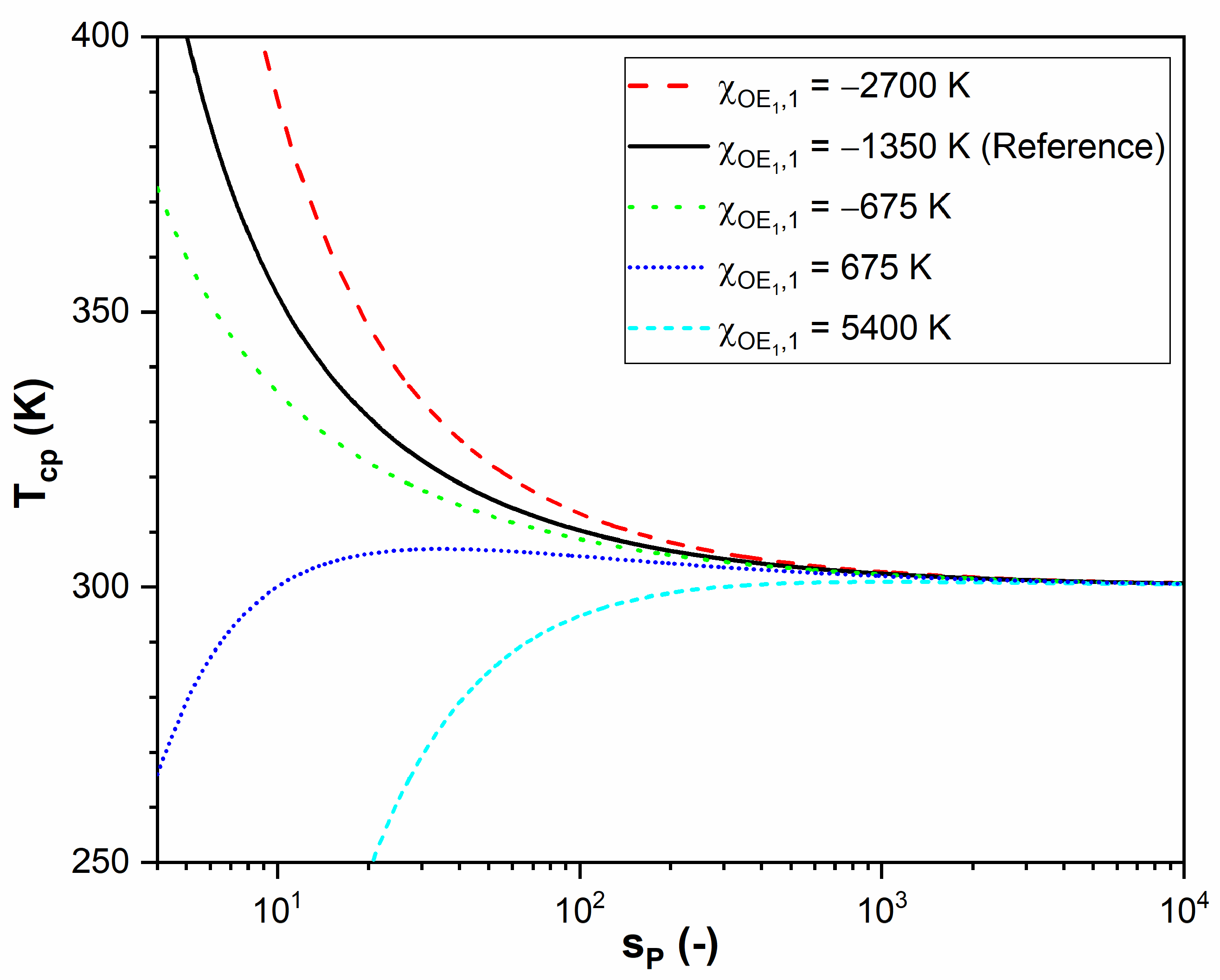
2.6. Theoretical Predictions of for a Hypothetical α-End-Functionalized Homopolymer
- the curve is the result for a polymer that has no distinct end segments (Case 1A).
- the end segment, compared to the middle segment, has a more favorable interaction with the solvent, and a steeper cloud point curve is obtained.
- the end segment, compared to the middle segment, has a less favorable interaction with the solvent, and the cloud point curve falls off more gently with .
- compared to the middle segment, the interaction of the solvent with the end segment worsens further; initially increases with , reaches a maximum, and subsequently reaches the asymptotic value , where the effect of the end group can be ignored.
- : increases asymptotically without a maximum to its limiting value at .
3. Application of FH Theory to Available Experimental Data
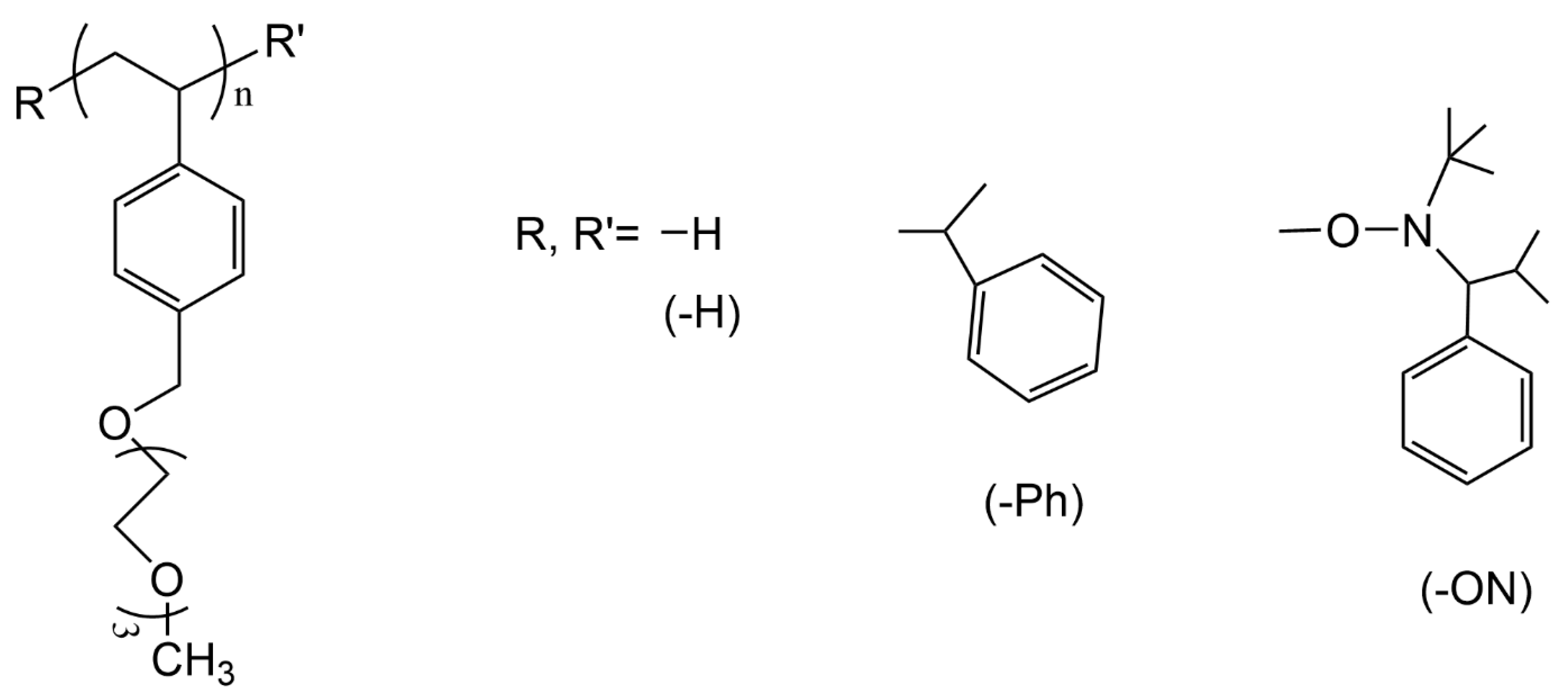
3.1. Selected Systems
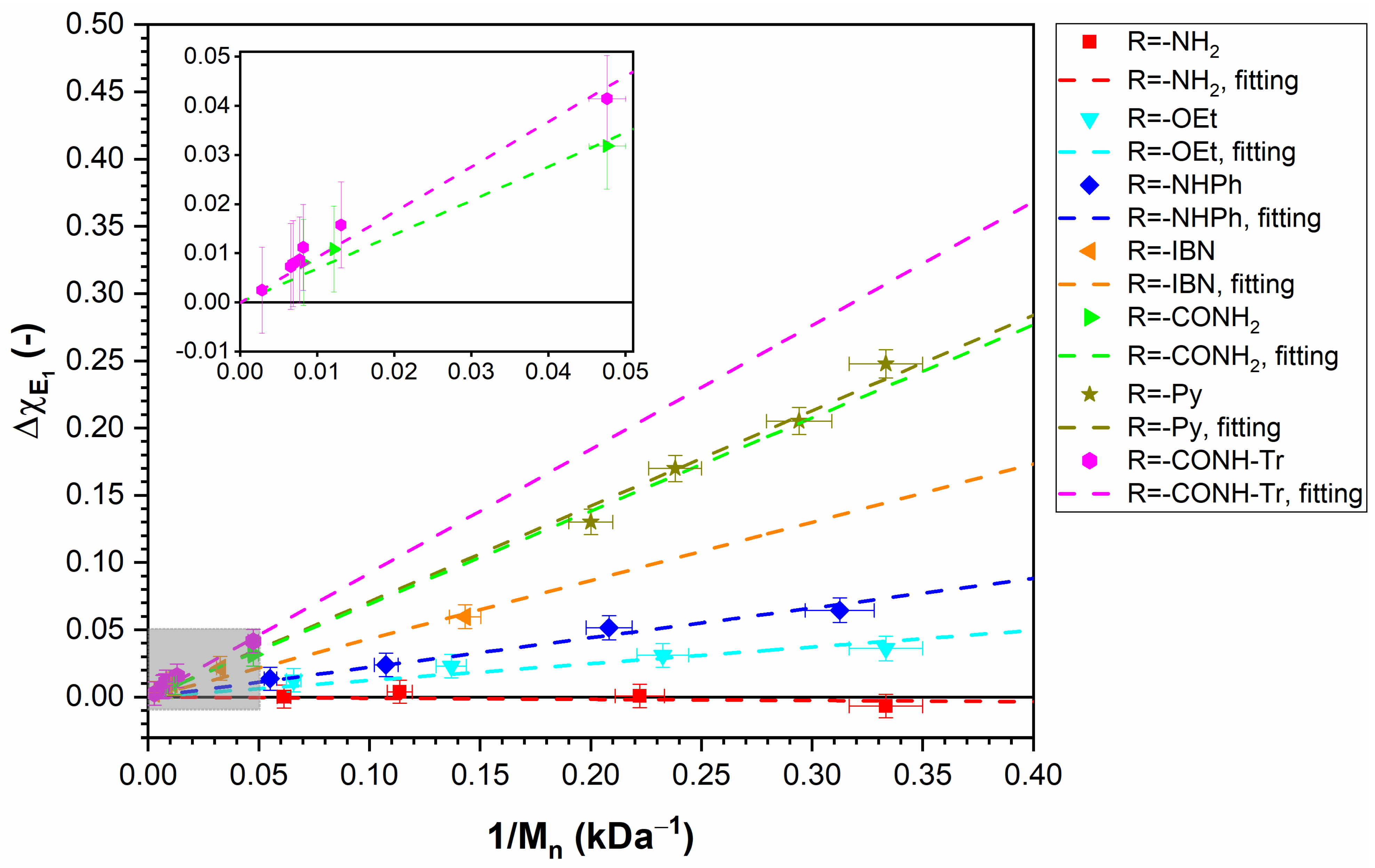
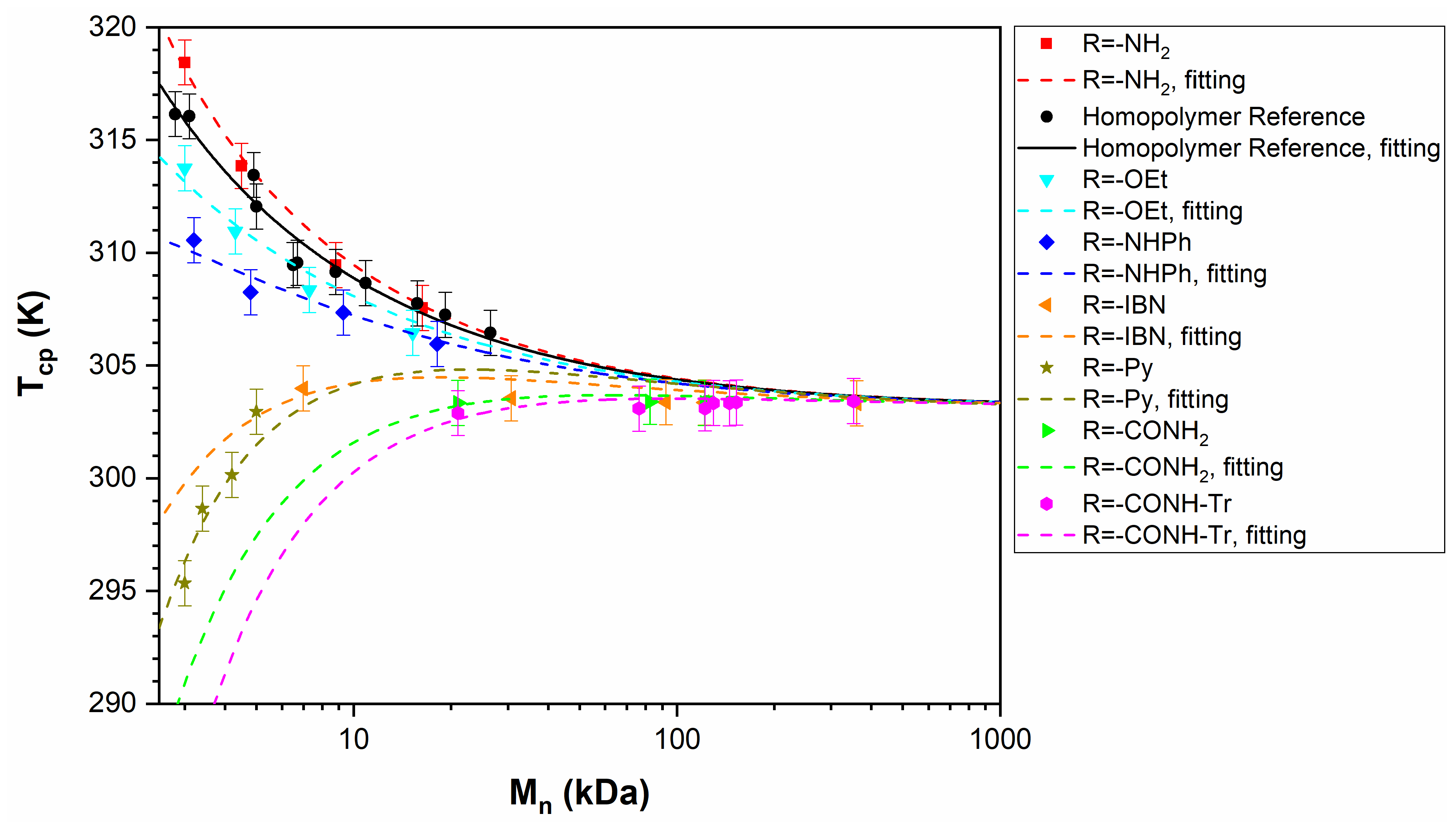
3.2. Relationships between Experimental Data and Theoretical Parameters
3.3. PNIPAM
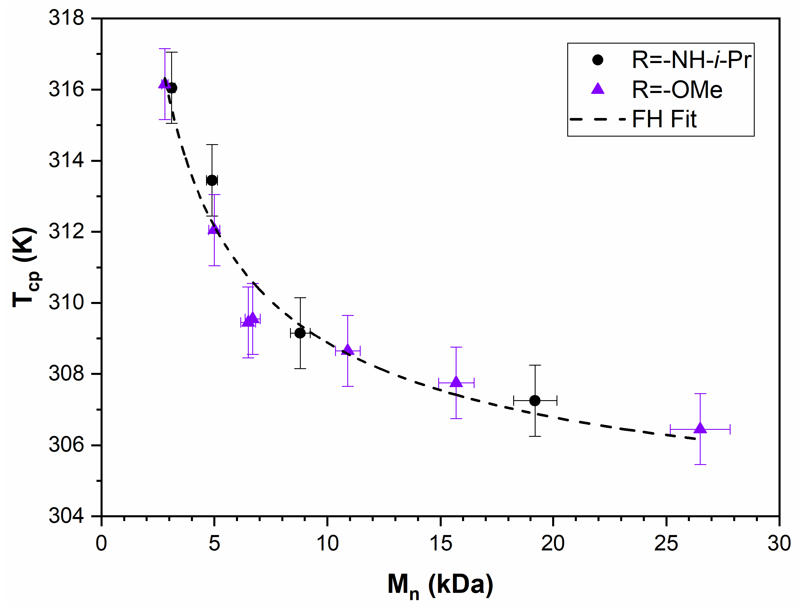
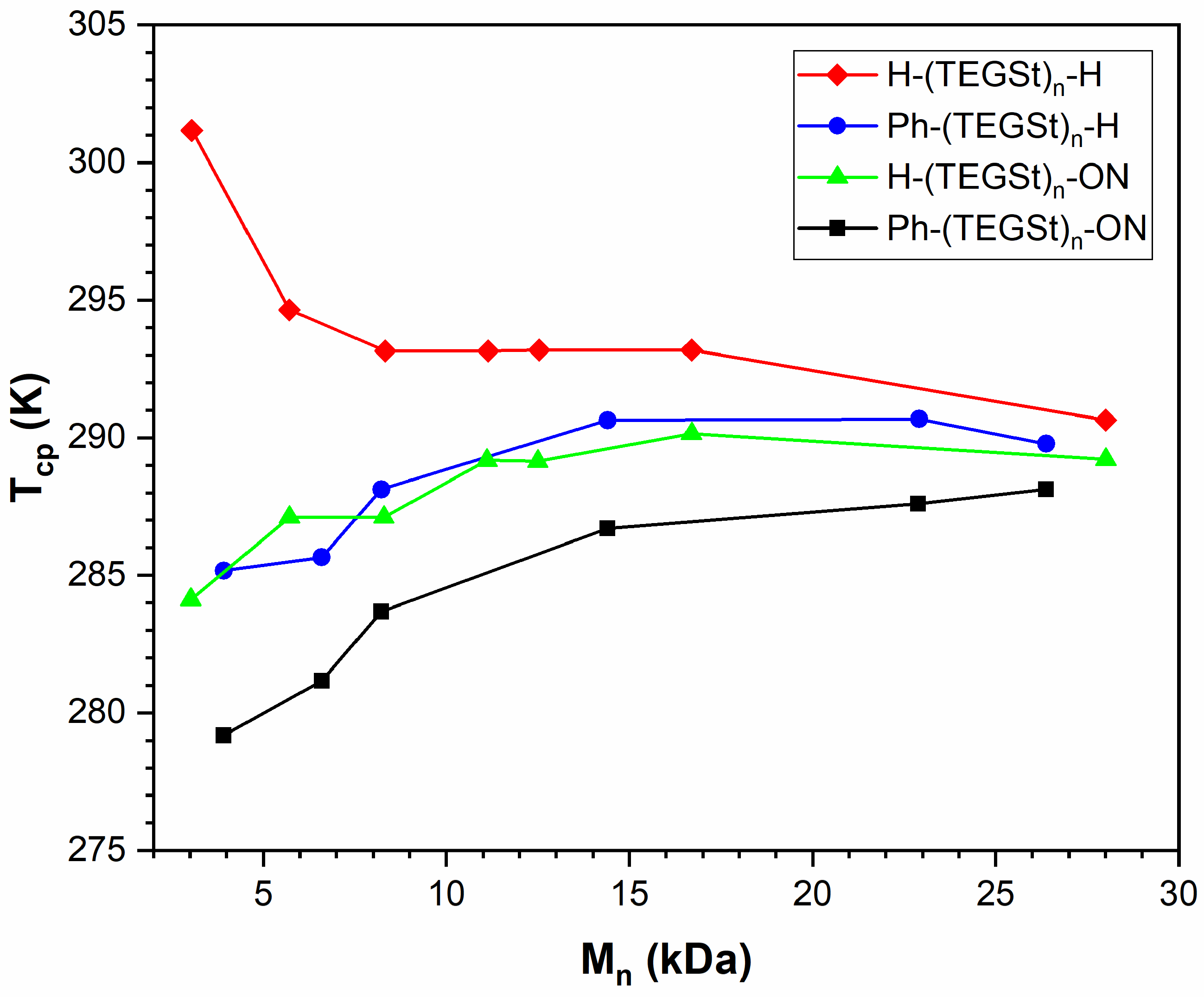
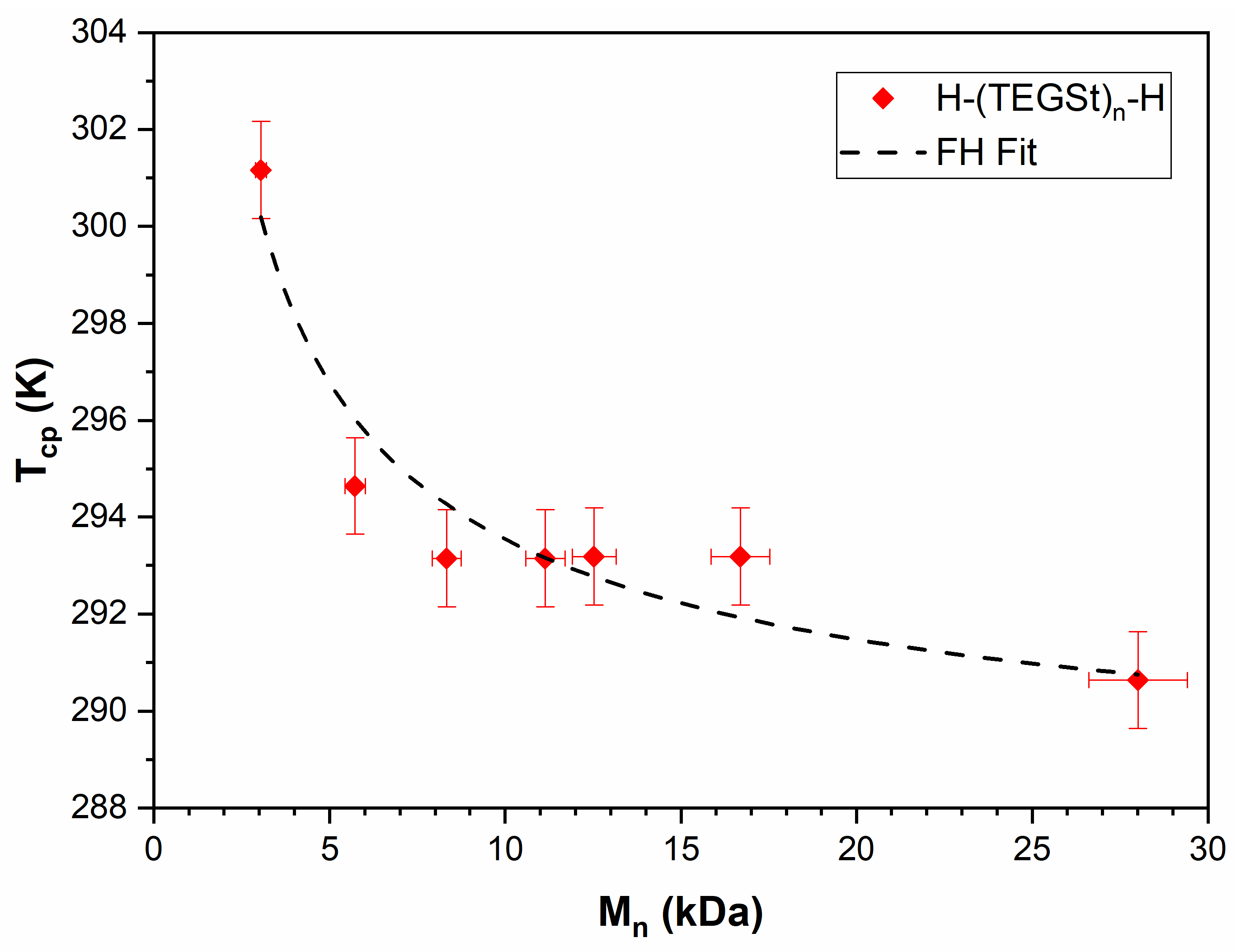
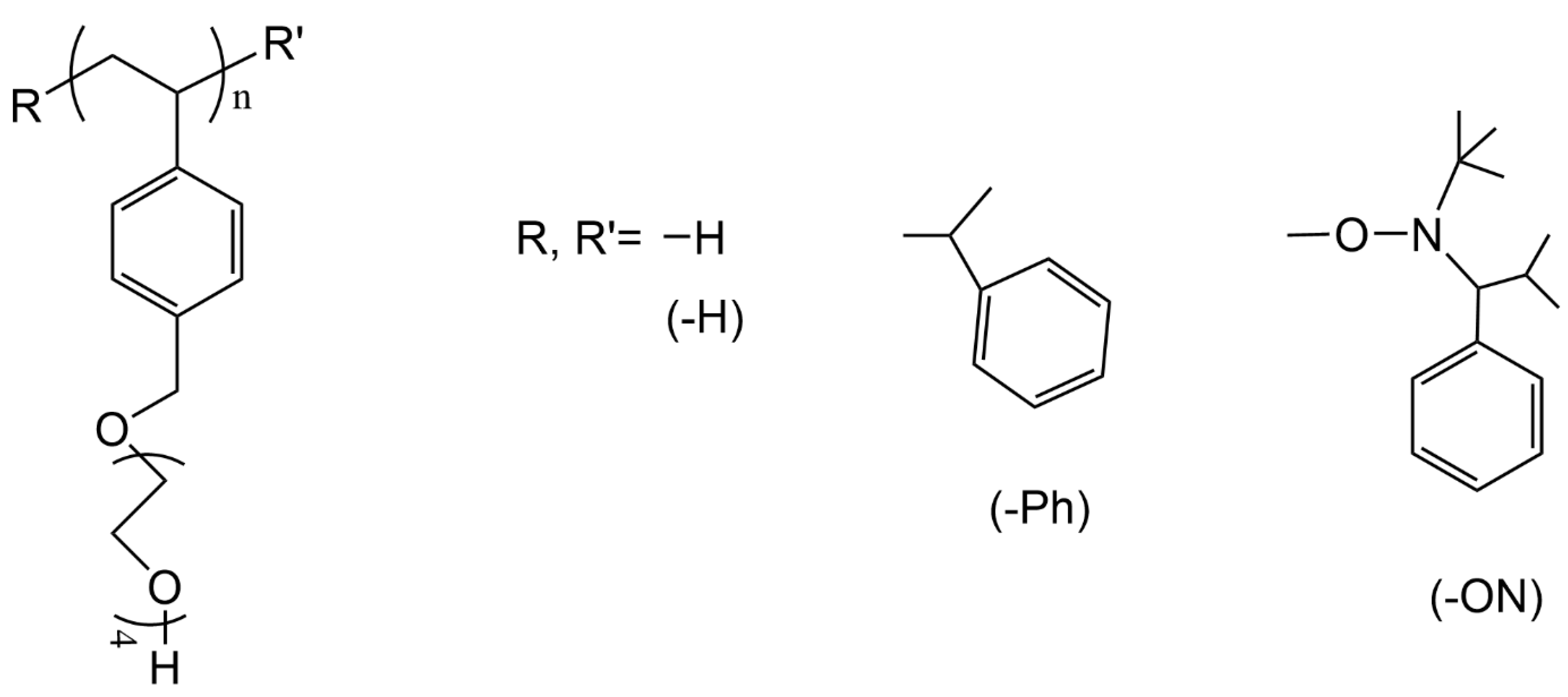
3.4. PTEGSt
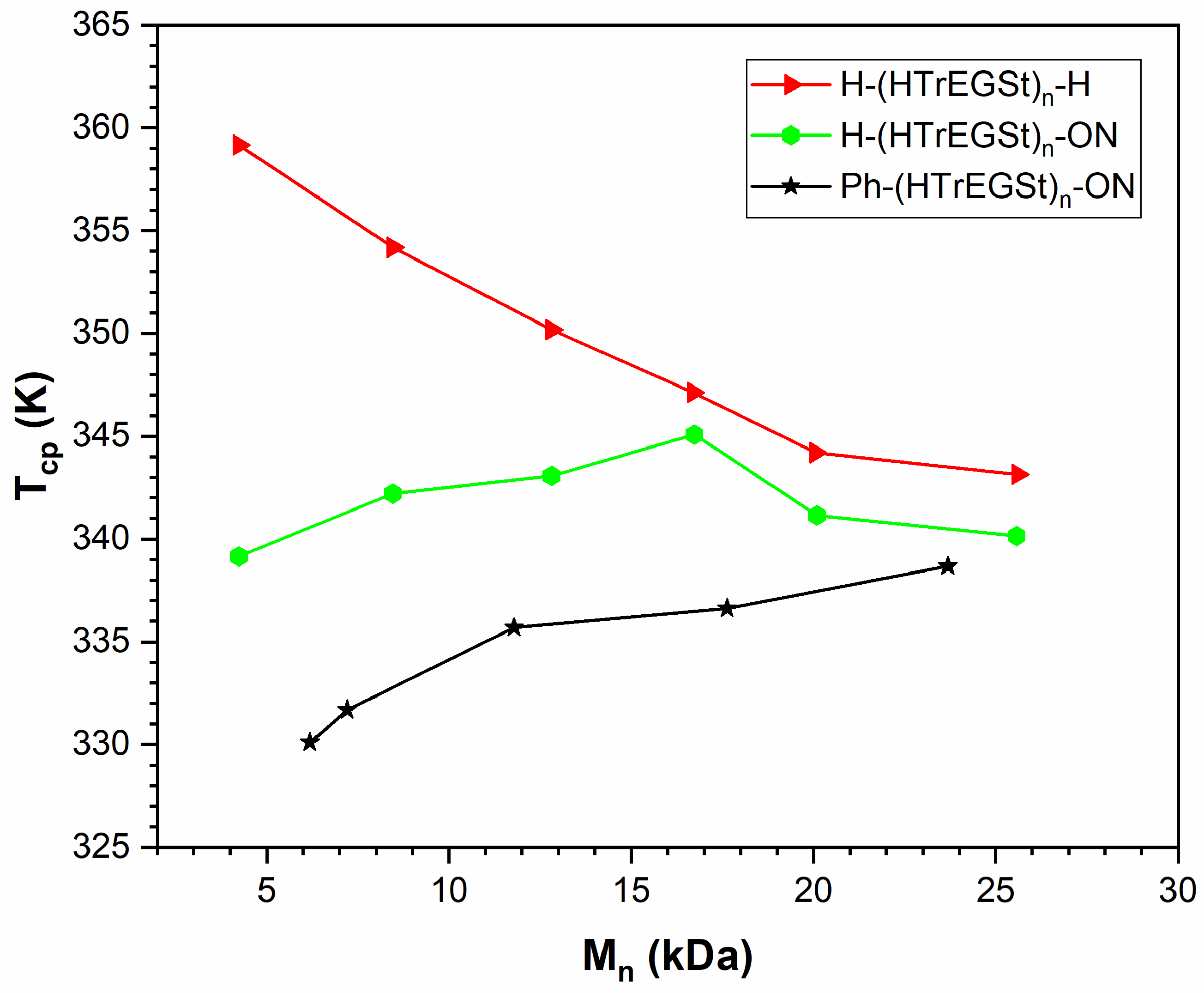
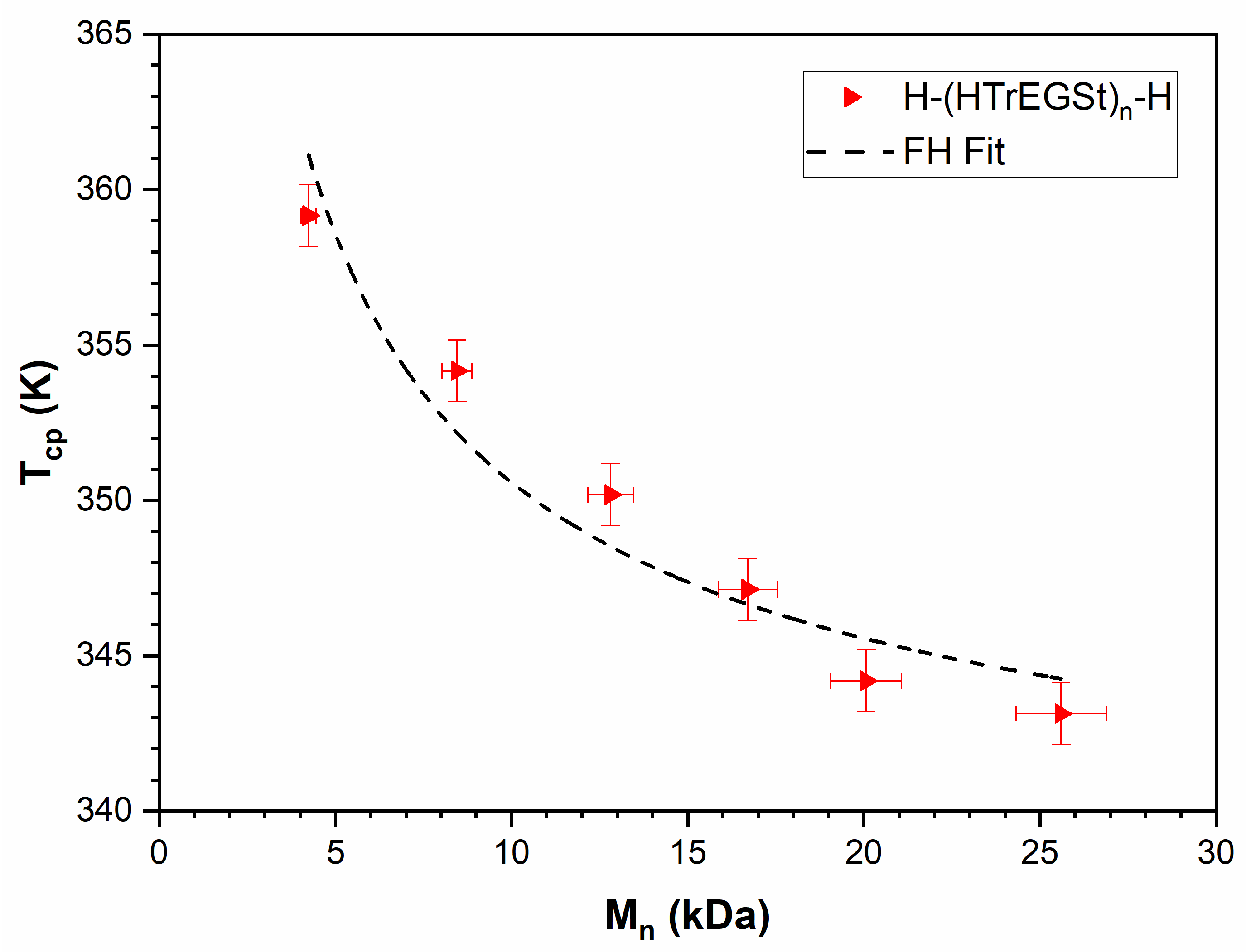
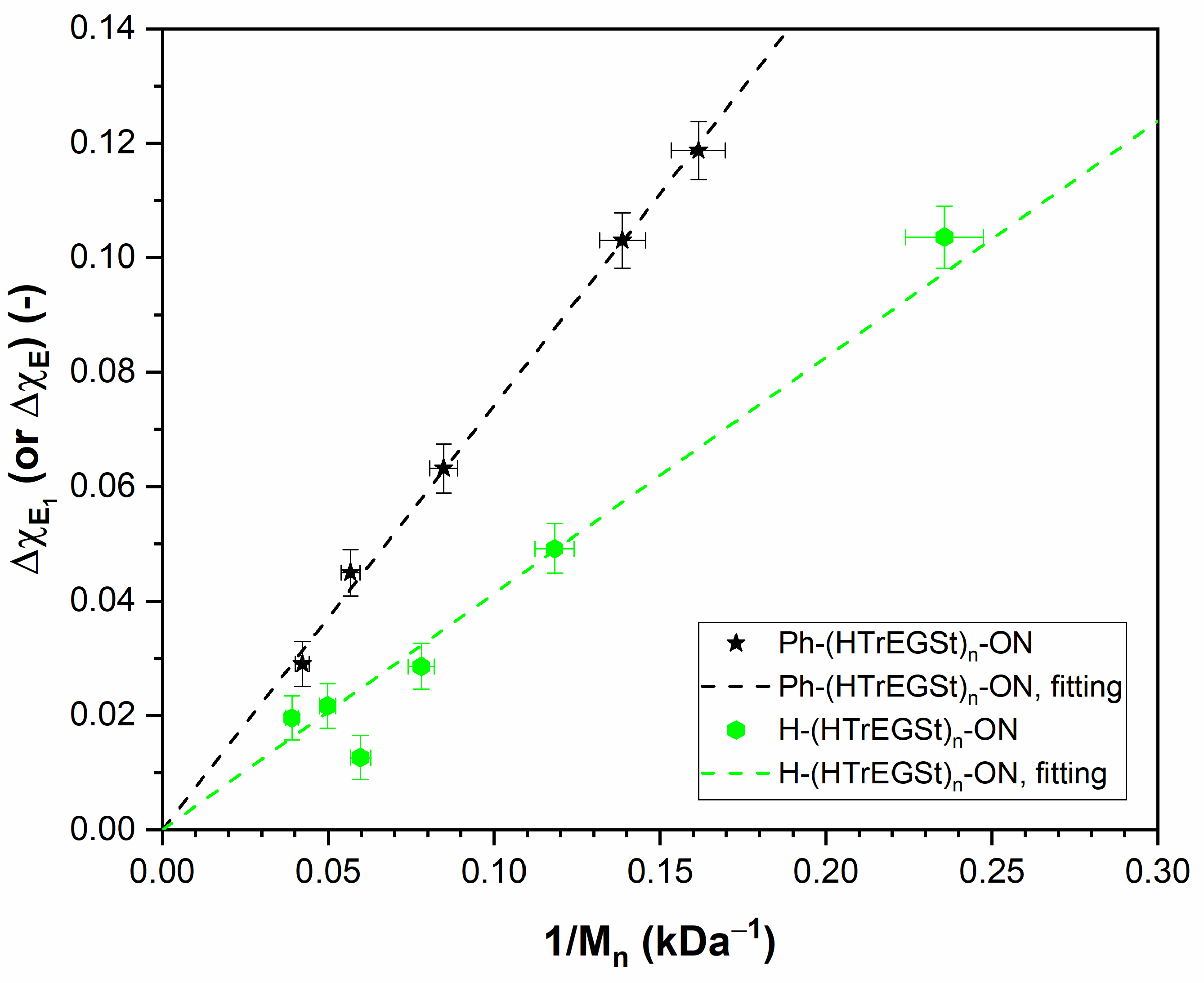
3.5. PHTrEGSt
4. Discussion
4.1. Summary of the Theoretical Results of the FH Theory and Comparison with Other Theories
4.2. The Theoretical Results of the FH Theory in Comparison with Experiments
4.3. Summary of the Theoretical Improvements to the FH Theory
4.4. Other Available Theories versus the Simple FH Theory for End-Functionalized Polymers
5. Conclusions
Supplementary Materials
Author Contributions
Funding
Institutional Review Board Statement
Data Availability Statement
Conflicts of Interest
Appendix A
Appendix A.1. FH Theory for Solutions of Linear Homopolymers without End Groups, Statistical Terpolymers, and α, ω–End-Functionalized Homopolymers
Appendix A.2. Lattice Theories beyond FH Theory for Linear Homopolymers without End Groups
Appendix A.2.1. Huggins, Guggenheim, and Lattice Cluster Theories
Appendix A.2.2. Lattice Cluster Theory for Linear Homopolymers (No Distinct End Groups) in Solvents
Appendix A.2.3. Relation between the LCT and the FH Theory
Appendix A.2.4. Relation between the LCT and the Huggins Theory
Appendix A.2.5. Relation between the LCT and the Guggenheim Theory
Appendix A.2.6. Relation between the Huggins Theory and the Guggenheim Theory
Appendix A.2.7. Estimate of the Effects of and on the FH Predictions
Appendix A.2.8. Summary of Improvements and Relation to the FH Theory
Appendix A.3. Statistical Terpolymers and End-Functionalized Homopolymers in a Solvent
Appendix A.3.1. Huggins and Linearized Guggenheim Theories
Appendix A.3.2. Nonrandom Mixing Guggenheim Theory
Appendix A.3.3. General Statement on the Effect of Nonrandom Mixing
Appendix A.3.4. Summary and Consequences of Improvements for the Functionalized Homopolymers
References
- Mukherji, D.; Marques, C.M.; Kremer, K. Smart Responsive Polymers: Fundamentals and Design Principles. Annu. Rev. Condens. Matter Phys. 2020, 11, 271–299. [Google Scholar] [CrossRef]
- Halperin, A.; Kröger, M.; Winnik, F.M. Poly(N-Isopropylacrylamide) Phase Diagrams: Fifty Years of Research. Angew. Chem. Int. Ed. 2015, 54, 15342–15367. [Google Scholar] [CrossRef] [PubMed]
- Roy, D.; Brooks, W.L.A.; Sumerlin, B.S. New Directions in Thermoresponsive Polymers. Chem. Soc. Rev. 2013, 42, 7214–7243. [Google Scholar] [CrossRef]
- Akiyama, H.; Tamaoki, N. Synthesis and Photoinduced Phase Transitions of Poly( N -Isopropylacrylamide) Derivative Functionalized with Terminal Azobenzene Units. Macromolecules 2007, 40, 5129–5132. [Google Scholar] [CrossRef]
- Hoare, T.; Pelton, R. Engineering Glucose Swelling Responses in Poly(N-Isopropylacrylamide)-Based Microgels. Macromolecules 2007, 40, 670–678. [Google Scholar] [CrossRef]
- Serizawa, T.; Wakita, K.; Akashi, M. Rapid Deswelling of Porous Poly(N-Isopropylacrylamide) Hydrogels Prepared by Incorporation of Silica Particles. Macromolecules 2002, 35, 10–12. [Google Scholar] [CrossRef]
- Raula, J.; Shan, J.; Nuopponen, M.; Niskanen, A.; Jiang, H.; Kauppinen, E.I.; Tenhu, H. Synthesis of Gold Nanoparticles Grafted with a Thermoresponsive Polymer by Surface-Induced Reversible-Addition-Fragmentation Chain-Transfer Polymerization. Langmuir 2003, 19, 3499–3504. [Google Scholar] [CrossRef]
- Ward, M.A.; Georgiou, T.K. Thermoresponsive Polymers for Biomedical Applications. Polymers 2011, 3, 1215–1242. [Google Scholar] [CrossRef]
- Sponchioni, M.; Capasso Palmiero, U.; Moscatelli, D. Thermo-Responsive Polymers: Applications of Smart Materials in Drug Delivery and Tissue Engineering. Mater. Sci. Eng. C 2019, 102, 589–605. [Google Scholar] [CrossRef]
- Tang, L.; Wang, L.; Yang, X.; Feng, Y.; Li, Y.; Feng, W. Poly(N-Isopropylacrylamide)-Based Smart Hydrogels: Design, Properties and Applications. Prog. Mater. Sci. 2021, 115, 100702. [Google Scholar] [CrossRef]
- Doberenz, F.; Zeng, K.; Willems, C.; Zhang, K.; Groth, T. Thermoresponsive Polymers and Their Biomedical Application in Tissue Engineering—A Review. J. Mater. Chem. B 2020, 8, 607–628. [Google Scholar] [CrossRef] [PubMed]
- Tong, Z.; Zeng, F.; Zheng, X.; Sato, T. Inverse Molecular Weight Dependence of Cloud Points for Aqueous Poly(N-Isopropylacrylamide) Solutions. Macromolecules 1999, 32, 4488–4490. [Google Scholar] [CrossRef]
- Xia, Y.; Yin, X.; Burke, N.A.D.; Stöver, H.D.H. Thermal Response of Narrow-Disperse Poly(N-Isopropylacrylamide) Prepared by Atom Transfer Radical Polymerization. Macromolecules 2005, 38, 5937–5943. [Google Scholar] [CrossRef]
- Hua, F.; Jiang, X.; Li, D.; Zhao, B. Well-Defined Thermosensitive, Water-Soluble Polyacrylates and Polystyrenics with Short Pendant Oligo(Ethylene Glycol) Groups Synthesized by Nitroxide-Mediated Radical Polymerization. J. Polym. Sci. Part A Polym. Chem. 2006, 44, 2454–2467. [Google Scholar] [CrossRef]
- De Oliveira, T.E.; Mukherji, D.; Kremer, K.; Netz, P.A. Effects of Stereochemistry and Copolymerization on the LCST of PNIPAm. J. Chem. Phys. 2017, 146, 034904. [Google Scholar] [CrossRef]
- Ray, B.; Okamoto, Y.; Kamigaito, M.; Sawamoto, M.; Seno, K.I.; Kanaoka, S.; Aoshima, S. Effect of Tacticity of Poly(N-Isopropylacrylamide) on the Phase Separation Temperature of Its Aqueous Solutions. Polym. J. 2005, 37, 234–237. [Google Scholar] [CrossRef]
- Xia, Y.; Burke, N.A.D.; Stöver, H.D.H. End Group Effect on the Thermal Response of Narrow-Disperse Poly(N-Isopropylacrylamide) Prepared by Atom Transfer Radical Polymerization. Macromolecules 2006, 39, 2275–2283. [Google Scholar] [CrossRef]
- Duan, Q.; Miura, Y.; Narumi, A.; Shen, X.; Sato, S.I.; Satoh, T.; Kakuchi, T. Synthesis and Thermoresponsive Property of End-Functionalized Poly(n-Isopropylacrylamide) with Pyrenyl Group. J. Polym. Sci. Part A Polym. Chem. 2006, 44, 1117–1124. [Google Scholar] [CrossRef]
- Van Durme, K.; Van Mele, B.; Bernaerts, K.V.; Verdonck, B.; Du Prez, F.E. End-Group Modified Poly(Methyl Vinyl Ether): Characterization and LCST Demixing Behavior in Water. J. Polym. Sci. Part B Polym. Phys. 2006, 44, 461–469. [Google Scholar] [CrossRef]
- Jiang, X.; Zhao, B. End Group Effect on the Thermo-Sensitive Properties of Well-Defined Water-Soluble Polystyrenics with Short Pendant Oligo(Ethylene Glycol) Groups Synthesized by Nitroxide-Mediated Radical Polymerization. J. Polym. Sci. Part A Polym. Chem. 2007, 45, 3707–3721. [Google Scholar] [CrossRef]
- Huber, S.; Hutter, N.; Jordan, R. Effect of End Group Polarity upon the Lower Critical Solution Temperature of Poly(2-Isopropyl-2-Oxazoline). Colloid Polym. Sci. 2008, 286, 1653–1661. [Google Scholar] [CrossRef]
- Roth, P.J.; Jochum, F.D.; Forst, F.R.; Zentel, R.; Theato, P. Influence of End Groups on the Stimulus-Responsive Behavior of Poly[Oligo(Ethylene Glycol) Methacrylate] in Water. Macromolecules 2010, 43, 4638–4645. [Google Scholar] [CrossRef]
- Narumi, A.; Fuchise, K.; Kakuchi, R.; Toda, A.; Satoh, T.; Kawaguchi, S.; Sugiyama, K.; Hirao, A.; Kakuchi, T. A Versatile Method for Adjusting Thermoresponsivity: Synthesis and “Click” Reaction of an Azido End-Functionalized Poly(N-Isopropylacrylamide). Macromol. Rapid Commun. 2008, 29, 1126–1133. [Google Scholar] [CrossRef]
- Qiu, X.; Koga, T.; Tanaka, F.; Winnik, F.M. New Insights into the Effects of Molecular Weight and End Group on the Temperature-Induced Phase Transition of Poly(N-Isopropylacrylamide) in Water. Sci. China Chem. 2013, 56, 56–64. [Google Scholar] [CrossRef]
- Zhang, Q.; Weber, C.; Schubert, U.S.; Hoogenboom, R. Thermoresponsive Polymers with Lower Critical Solution Temperature: From Fundamental Aspects and Measuring Techniques to Recommended Turbidimetry Conditions. Mater. Horiz. 2017, 4, 109–116. [Google Scholar] [CrossRef]
- Chung, J.E.; Yokoyama, M.; Aoyagi, T.; Sakurai, Y.; Okano, T. Effect of Molecular Architecture of Hydrophobically Modified Poly(N-Isopropylacrylamide) on the Formation of Thermoresponsive Core-Shell Micellar Drug Carriers. J. Control. Release 1998, 53, 119–130. [Google Scholar] [CrossRef]
- Plummer, R.; Hill, D.J.T.; Whittaker, A.K. Solution Properties of Star and Linear Poly(N-Isopropylacrylamide). Macromolecules 2006, 39, 8379–8388. [Google Scholar] [CrossRef]
- Miasnikova, A.; Laschewsky, A. Influencing the Phase Transition Temperature of Poly(Methoxy Diethylene Glycol Acrylate) by Molar Mass, End Groups, and Polymer Architecture. J. Polym. Sci. Part A Polym. Chem. 2012, 50, 3313–3323. [Google Scholar] [CrossRef]
- Furyk, S.; Zhang, Y.; Ortiz-Acosta, D.; Cremer, P.S.; Bergbreiter, D.E. Effects of End Group Polarity and Molecular Weight on the Lower Critical Solution Temperature of Poly(N-Isopropylacrylamide). J. Polym. Sci. Part A Polym. Chem. 2006, 44, 1492–1501. [Google Scholar] [CrossRef]
- Kujawa, P.; Segui, F.; Shaban, S.; Diab, C.; Okada, Y.; Tanaka, F.; Winnik, F.M. Impact of End-Group Association and Main-Chain Hydration on the Thermosensitive Properties of Hydrophobically Modified Telechelic Poly(N-Isopropylacrylamides) in Water. Macromolecules 2006, 39, 341–348. [Google Scholar] [CrossRef]
- Fujishige, S.; Kubota, K.; Ando, I. Phase Transition of Aqueous Solutions of Poly(N-Isopropylacrylamide) and Poly(N-Isopropylmethacrylamide). J. Phys. Chem. 1989, 93, 3311–3313. [Google Scholar] [CrossRef]
- Huggins, M.L. Solutions of Long Chain Compounds. J. Chem. Phys. 1941, 9, 440. [Google Scholar] [CrossRef]
- Huggins, M.L. Thermodynamics Properties of Solutions of Long-Chain Compounds. Ann. N. Y. Acad. Sci. 1942, 43, 1–32. [Google Scholar] [CrossRef]
- Flory, P.J. Thermodynamics of High Polymer Solutions. J. Chem. Phys. 1942, 10, 51–61. [Google Scholar] [CrossRef]
- Flory, P.J. Thermodynamics of High Polymer Solutions. J. Chem. Phys. 1941, 9, 660–661. [Google Scholar] [CrossRef]
- Koningsveld, R.; Stockmayer, W.H.; Nies, E. Demixing of Strictly Binary Systems. In Polymer Phase Diagrams: A Textbook; Oxford University Press: Oxford, UK, 2001; pp. 122–125. ISBN 978-0198556343. [Google Scholar]
- Flory, P.J. Experimental Results on Binary Systems. In Principles of Polymer Chemistry; Cornell University Press: Ithaca, NY, USA, 1953; pp. 546–548. ISBN 978-0801401343. [Google Scholar]
- Duan, Q.; Narumi, A.; Miura, Y.; Shen, X.; Sato, S.I.; Satoh, T.; Kakuchi, T. Thermoresponsive Property Controlled by End-Functionalization of Poly(N-Isopropylacrylamide) with Phenyl, Biphenyl, and Triphenyl Groups. Polym. J. 2006, 38, 306–310. [Google Scholar] [CrossRef]
- Chung, J.E.; Yokoyama, M.; Suzuki, K.; Aoyagi, T.; Sakurai, Y.; Okano, T. Reversibly Thermo-Responsive Alkyl-Terminated Poly(N-Isopropylacrylamide) Core-Shell Micellar Structures. Colloids Surf. B Biointerfaces 1997, 9, 37–48. [Google Scholar] [CrossRef]
- Winnik, F.M.; Davidson, A.R.; Hamer, G.K.; Kitano, H. Amphiphilic Poly(N-Isopropylacrylamides) Prepared by Using a Lipophilic Radical Initiator: Synthesis and Solution Properties in Water. Macromolecules 1992, 25, 1876–1880. [Google Scholar] [CrossRef]
- Koningsveld, R.; Stockmayer, W.H.; Nies, E. Molecular Basis of the Interaction Parameter. In Polymer Phase Diagrams: A Textbook; Oxford University Press: Oxford, UK, 2001; pp. 282–284. ISBN 978-0198556343. [Google Scholar]
- Delmas, G.; Patterson, D.; Somcynsky, T. Thermodynamics of Polyisobutylene–n-Alkane Systems. J. Polym. Sci. 1962, 57, 79–98. [Google Scholar] [CrossRef]
- Shultz, A.R.; Flory, P.J. Phase Equilibria in Polymer-Solvent Systems. II. Thermodynamic Interaction Parameters from Critical Miscibility Data. J. Am. Chem. Soc. 1953, 75, 3888–3892. [Google Scholar] [CrossRef]
- Simha, R.; Branson, H. Theory of Chain Copolymerization Reactions. J. Chem. Phys. 1944, 12, 253–267. [Google Scholar] [CrossRef]
- Stockmayer, W.H.; Moore, L.D.; Fixman, M.; Epstein, B.N. Copolymers in Dilute Solution. I. Preliminary Results for Styrene-Methyl Methacrylate. J. Polym. Sci. 1955, 16, 517–530. [Google Scholar] [CrossRef]
- Kilb, R.W.; Bueche, A.M. Solution and Fractionation Properties of Graft Polymers. J. Polym. Sci. 1958, 28, 285–294. [Google Scholar] [CrossRef]
- Krause, S. Note on a Paper by Kilb and Bueche on Solution and Fractionation Properties of Graft Polymers. J. Polym. Sci. 1959, 35, 558–559. [Google Scholar] [CrossRef]
- Krause, S.; Smith, A.L.; Duden, M.G. Polymer Mixtures Including Random Copolymers. Zeroth Approximation. J. Chem. Phys. 1965, 43, 2144–2145. [Google Scholar] [CrossRef]
- Origin Graphing & Analysis; Version 2018b; OriginLab Corporation: Northampton, MA, USA, 2018.
- Hillegers, L.T.M.E. The Estimation of Parameters in Functional Relationship Models. Ph.D. Thesis, Eindhoven University of Technology, Eindhoven, The Netherlands, 1986. [Google Scholar]
- Madden, W.G.; Pesci, A.I.; Freed, K.F. Phase Equilibria of Lattice Polymer and Solvent: Tests of Theories against Simulations. Macromolecules 1990, 23, 1181–1191. [Google Scholar] [CrossRef]
- Orr, W.J.C. The Free Energies of Solutions of Single and Multiple Molecules. Trans. Faraday Soc. 1944, 40, 320–332. [Google Scholar] [CrossRef]
- Guggenheim, E.A. Statistical Thermodynamics of Mixtures with Zero Energies of Mixing. Proc. R. Soc. Lond. Ser. A Math. Phys. Sci. 1944, 183, 203–212. [Google Scholar] [CrossRef]
- Guggenheim, E.A. Statistical Thermodynamics of Mixtures with Non-Zero Energies of Mixing. Proc. R. Soc. Lond. Ser. A Math. Phys. Sci. 1944, 183, 213–227. [Google Scholar] [CrossRef]
- Guggenheim, E.A. Mixtures; Oxford University Press: Oxford, UK, 1952. [Google Scholar]
- Miller, A.R. The Number of Configurations of a Cooperative Assembly. Math. Proc. Camb. Philos. Soc. 1942, 38, 109–124. [Google Scholar] [CrossRef]
- Miller, A.R. The Vapour-Pressure Equations of Solutions and the Osmotic Pressure of Rubber. Math. Proc. Camb. Philos. Soc. 1943, 39, 54–67. [Google Scholar] [CrossRef]
- Dudowicz, J.; Freed, K.F.; Madden, W.G. Role of Molecular Structure on the Thermodynamic Properties of Melts, Blends, and Concentrated Polymer Solutions: Comparison of Monte Carlo Simulations with the Cluster Theory for the Lattice Model. Macromolecules 1990, 23, 4803–4819. [Google Scholar] [CrossRef]
- Freed, K.F. New Lattice Model for Interacting, Avoiding Polymers with Controlled Length Distribution. J. Phys. A Math. Gen. 1985, 18, 871–877. [Google Scholar] [CrossRef]
- Bawendi, M.G.; Freed, K.F. Statistical Mechanics of the Packing of Rods on a Lattice: Cluster Expansion for Systematic Corrections to Mean Field. J. Chem. Phys. 1986, 85, 3007–3022. [Google Scholar] [CrossRef]
- Bawendi, M.G.; Freed, K.F. Systematic Corrections to Flory–Huggins Theory: Polymer–Solvent–Void Systems and Binary Blend–Void Systems. J. Chem. Phys. 1988, 88, 2741–2756. [Google Scholar] [CrossRef]
- Bawendi, M.G.; Freed, K.F.; Mohanty, U. A Lattice Field Theory for Polymer Systems with Nearest-Neighbor Interaction Energies. J. Chem. Phys. 1987, 87, 5534–5540. [Google Scholar] [CrossRef]
- Pesci, A.I.; Freed, K.F. Lattice Models of Polymer Fluids: Monomers Occupying Several Lattice Sites. II. Interaction Energies. J. Chem. Phys. 1989, 90, 2003–2016. [Google Scholar] [CrossRef]
- Pesci, A.I.; Freed, K.F. Lattice Theory of Polymer Blends and Liquid Mixtures: Beyond the Flory–Huggins Approximation. J. Chem. Phys. 1989, 90, 2017–2026. [Google Scholar] [CrossRef]
- Nemirovsky, A.M.; Bawendi, M.G.; Freed, K.F. Lattice Models of Polymer Solutions: Monomers Occupying Several Lattice Sites. J. Chem. Phys. 1987, 87, 7272–7284. [Google Scholar] [CrossRef]
- Bawendi, M.G.; Freed, K.F.; Mohanty, U. A Lattice Model for Self-Avoiding Polymers with Controlled Length Distributions. II. Corrections to Flory–Huggins Mean Field. J. Chem. Phys. 1986, 84, 7036–7047. [Google Scholar] [CrossRef]
- Freed, K.F.; Pesci, A.I. Theory of the Molecular Origins of the Entropic Portion of the Flory χ Parameter for Polymer Blends. J. Chem. Phys. 1987, 87, 7342–7344. [Google Scholar] [CrossRef]
- Freed, K.F.; Bawendi, M.G. Lattice Theories of Polymeric Fluids. J. Phys. Chem. 1989, 93, 2194–2203. [Google Scholar] [CrossRef]
- Cifra, P.; Nies, E.; Broersma, J. Equation of State and Miscibility Behavior of Compressible Binary Lattice Polymers. A Monte Carlo Study and Comparison with Partition Function Theories. Macromolecules 1996, 29, 6634–6644. [Google Scholar] [CrossRef]
- Wang, S.; Nies, E.; Cifra, P. A Theory for Compressible Binary Lattice Polymers: Influence of Chain Conformational Properties. J. Chem. Phys. 1998, 109, 5639–5650. [Google Scholar] [CrossRef]
- Hagemark, K. Thermodynamics of Ternary Systems. Quasi-Chemical Approximation. J. Phys. Chem. 1968, 72, 2316–2322. [Google Scholar] [CrossRef]
- Hagemark, K.I. Thermodynamics of Multicomponent Systems. The Quasichemical Approximation. J. Chem. Phys. 1973, 59, 2344–2346. [Google Scholar] [CrossRef]
- Hagemark, K.I. Thermodynamics of Ternary Systems. Quasichemical Approximation and the Excess Ternary Term. J. Chem. Phys. 1974, 61, 2596–2599. [Google Scholar] [CrossRef]
- Kumar, S.K.; Suter, U.W.; Reid, R.C. A Statistical Mechanics Based Lattice Model Equation of State. Ind. Eng. Chem. Res. 1987, 26, 2532–2542. [Google Scholar] [CrossRef]
- Okada, Y.; Tanaka, F.; Kujawa, P.; Winnik, F.M. Unified Model of Association-Induced Lower Critical Solution Temperature Phase Separation and Its Application to Solutions of Telechelic Poly(Ethylene Oxide) and of Telechelic Poly(N-Isopropylacrylamide) in Water. J. Chem. Phys. 2006, 125, 244902. [Google Scholar] [CrossRef] [PubMed]
- Kojima, H.; Tanaka, F. Nonlinear Depression of the Lower Critical Solution Temperatures in Aqueous Solutions of Thermo-sensitive Random Copolymers. J. Polym. Sci. Part B Polym. Phys. 2013, 51, 1112–1123. [Google Scholar] [CrossRef]
- Gross, J.; Sadowski, G. Perturbed-Chain SAFT: An Equation of State Based on a Perturbation Theory for Chain Molecules. Ind. Eng. Chem. Res. 2001, 40, 1244–1260. [Google Scholar] [CrossRef]
- Gross, J.; Sadowski, G. Application of the Perturbed-Chain SAFT Equation of State to Associating Systems. Ind. Eng. Chem. Res. 2002, 41, 5510–5515. [Google Scholar] [CrossRef]
- Chapman, W.G.; Gubbins, K.E.; Jackson, G.; Radosz, M. New Reference Equation of State for Associating Liquids. Ind. Eng. Chem. Res. 1990, 29, 1709–1721. [Google Scholar] [CrossRef]
- Wertheim, M.S. Fluids with Highly Directional Attractive Forces. I. Statistical Thermodynamics. J. Stat. Phys. 1984, 35, 19–34. [Google Scholar] [CrossRef]
- Wertheim, M.S. Fluids with Highly Directional Attractive Forces. II. Thermodynamic Perturbation Theory and Integral Equations. J. Stat. Phys. 1984, 35, 35–47. [Google Scholar] [CrossRef]
- Wertheim, M.S. Fluids with Highly Directional Attractive Forces. III. Multiple Attraction Sites. J. Stat. Phys. 1986, 42, 459–476. [Google Scholar] [CrossRef]
- Wertheim, M.S. Fluids with Highly Directional Attractive Forces. IV. Equilibrium Polymerization. J. Stat. Phys. 1986, 42, 477–492. [Google Scholar] [CrossRef]
- Arndt, M.C.; Sadowski, G. Modeling Poly(N-Isopropylacrylamide) Hydrogels in Water/Alcohol Mixtures with PC-SAFT. Macromolecules 2012, 45, 6686–6696. [Google Scholar] [CrossRef]
- Valsecchi, M.; Galindo, A.; Jackson, G. Modelling the Thermodynamic Properties of the Mixture of Water and Polyethylene Glycol (PEG) with the SAFT-γ Mie Group-Contribution Approach. Fluid Phase Equilibria 2024, 577, 113952. [Google Scholar] [CrossRef]
- Dudowicz, J.; Freed, K.F. Effect of Monomer Structure and Compressibility on the Properties of Multicomponent Polymer Blends and Solutions: 1. Lattice Cluster Theory of Compressible Systems. Macromolecules 1991, 24, 5076–5095. [Google Scholar] [CrossRef]
- Buta, D.; Freed, K.F. Mixtures of Lattice Polymers with Structured Monomers. J. Chem. Phys. 2004, 120, 6288–6298. [Google Scholar] [CrossRef]
- Dudowicz, J.; Freed, M.S.; Freed, K.F. Effect of Monomer Structure and Compressibility on the Properties of Multicomponent Polymer Blends and Solutions. 2. Application to Binary Blends. Macromolecules 1991, 24, 5096–5111. [Google Scholar] [CrossRef]
- Freed, K.F.; Dudowicz, J. Role of Monomer Structure and Compressibility on the Properties of Multicomponent Polymer Blends and Solutions. Theor. Chim. Acta 1992, 82, 357–382. [Google Scholar] [CrossRef]
- Dudowicz, J.; Freed, K.F. Relation of Effective Interaction Parameters for Binary Blends and Diblock Copolymers: Lattice Cluster Theory Predictions and Comparisons with Experiment. Macromolecules 1993, 26, 213–220. [Google Scholar] [CrossRef]
- Dudowicz, J.; Freed, K.F. Lattice Cluster Theory for Pedestrian. 2. Random Copolymer Systems. Macromolecules 2000, 33, 3467–3477. [Google Scholar] [CrossRef]
- Freed, K.F.; Dudowicz, J. Lattice Cluster Theory for Pedestrians: Models for Random Copolymer Blends. Macromol. Symp. 2000, 149, 11–16. [Google Scholar] [CrossRef]
- Dudowicz, J.; Freed, K.F. Lattice Cluster Theory of Associating Polymers. I. Solutions of Linear Telechelic Polymer Chains. J. Chem. Phys. 2012, 136, 064902. [Google Scholar] [CrossRef]
- Dudowicz, J.; Freed, K.F.; Douglas, J.F. Lattice Cluster Theory of Associating Polymers. II. Enthalpy and Entropy of Self-Assembly and Flory-Huggins Interaction Parameter χ for Solutions of Telechelic Molecules. J. Chem. Phys. 2012, 136, 064903. [Google Scholar] [CrossRef] [PubMed]
- Dudowicz, J.; Freed, K.F.; Douglas, J.F. Lattice Cluster Theory of Associating Polymers. IV. Phase Behavior of Telechelic Polymer Solutions. J. Chem. Phys. 2012, 136, 194903. [Google Scholar] [CrossRef]
- Nies, E.; Koningsveld, R.; Kleintjens, L.A. On Polymer Solution Thermodynamics. In Frontiers in Polymer Science; Steinkopff: Darmstadt, Germany, 1985; Volume 71, pp. 2–14. [Google Scholar]
- Foreman, K.W.; Freed, K.F. Generalizations of Huggins–Guggenheim–Miller-Type Theories to Describe the Architecture of Branched Lattice Chains. J. Chem. Phys. 1995, 102, 4663–4672. [Google Scholar] [CrossRef]


| B0 | B1 | B2 | B3 | B4 | B5 | B6 | ||
|---|---|---|---|---|---|---|---|---|
| 0.05 | 0.517318 | 0.4415 | −0.87889 | 0.16559 | −0.08219 | 0.02766 | −0.0061 | 5.24856 × 10⁻⁴ |
| 0.01 | 0.503359 | 0.62228 | −0.89899 | 0.12377 | −0.01639 | −0.00327 | 0.00108 | −9.87525 × 10⁻⁵ |
| 0.005 | 0.501673 | 0.6859 | −0.91305 | 0.12385 | −0.01107 | −0.00516 | 0.00141 | −1.15139 × 10⁻⁴ |
| 0.001 | 0.500334 | 0.80834 | −0.93836 | 0.11805 | 0.00151 | −0.00946 | 0.00209 | −1.52861 × 10⁻⁴ |
| R Groups | Coefficients |
|---|---|
| (kDa) | |
| -NH2 | −0.008 ± 0.009 |
| -OEt | 0.12 ± 0.01 |
| -NHPh | 0.22 ± 0.01 |
| -IBN | 0.43 ± 0.04 |
| -CONH2 | 0.69 ± 0.05 |
| -Py | 0.71 ± 0.02 |
| -CONH-Tr | 0.92 ± 0.05 |
| End Groups | Coefficients |
|---|---|
| (kDa) | |
| -Ph | 0.47 ± 0.04 (fitted) |
| -ON | 0.53 ± 0.02 (fitted) |
| -Ph and -ON | 1.00 ± 0.05 (predicted) |
| End Groups | Coefficients |
|---|---|
| (kDa) | |
| -ON | 0.41 ± 0.03 (fitted) |
| -Ph and -ON | 0.74 ± 0.01 (fitted) |
| -Ph | 0.33 ± 0.03 (predicted) |
Disclaimer/Publisher’s Note: The statements, opinions and data contained in all publications are solely those of the individual author(s) and contributor(s) and not of MDPI and/or the editor(s). MDPI and/or the editor(s) disclaim responsibility for any injury to people or property resulting from any ideas, methods, instructions or products referred to in the content. |
© 2024 by the authors. Licensee MDPI, Basel, Switzerland. This article is an open access article distributed under the terms and conditions of the Creative Commons Attribution (CC BY) license (https://creativecommons.org/licenses/by/4.0/).
Share and Cite
Dang, T.T.N.; Nies, E. Effect of End Groups on the Cloud Point Temperature of Aqueous Solutions of Thermoresponsive Polymers: An Inside View by Flory–Huggins Theory. Polymers 2024, 16, 563. https://doi.org/10.3390/polym16040563
Dang TTN, Nies E. Effect of End Groups on the Cloud Point Temperature of Aqueous Solutions of Thermoresponsive Polymers: An Inside View by Flory–Huggins Theory. Polymers. 2024; 16(4):563. https://doi.org/10.3390/polym16040563
Chicago/Turabian StyleDang, Thi To Nga, and Erik Nies. 2024. "Effect of End Groups on the Cloud Point Temperature of Aqueous Solutions of Thermoresponsive Polymers: An Inside View by Flory–Huggins Theory" Polymers 16, no. 4: 563. https://doi.org/10.3390/polym16040563