Abstract
Size-exclusion chromatography (SEC) is presently a widely used and very informative technique for the characterization of macromolecules in solution. Beyond the first implementations of SEC—which required cumbersome column calibrations and were mainly intended for the determination of molecular weights—the modern SEC approach involving multiple detectors (md-SEC) is based on solution properties such as intrinsic viscosity and light scattering. Thus, md-SEC enables the direct and more efficient determination of molecular weights, as well as the determination of relationships between property and molecular weight, which can be quite useful in structural studies. Here, we first present a review of the fundamental aspects of the dilute-solution properties of macromolecules—particularly the differential refractive index, intrinsic viscosity, and scattering-related properties—on which the various detectors involved in md-SEC are based. Then, we developed SECtools, a suite of public-domain, open-source computer programs, which allow for the full analysis of md-SEC chromatograms. These analyses range from just the recorded raw signals (mV) of the detectors to a full determination of molecular weight averages and distributions. The use of these programs is illustrated through experimental studies using various samples.
1. Introduction
The most essential aspect of the characterization of macromolecular compounds is the determination of their molecular weight, M. Furthermore, in many cases, the sample is polydisperse, containing macromolecules with various (a few or many) species with varying M. Then, the characterization would consist of the determination of the molecular weight distribution or, at least, the molecular weight averages and degree of polydispersity. Another essential aspect is the elucidation of the global conformation (shape or flexibility) of the macromolecular chains, which is usually performed by studying the molecular weight dependence of properties in solution—either hydrodynamic quantities such as the intrinsic viscosity, , or other quantities obtained from scattering techniques like the radius of gyration [1,2].
These purposes require the fractionation of the sample into some number of fractions with different (narrower) ranges of size, which would be later individually characterized to obtain some estimate of their approximate or average M, typically from static scattering or from some known property vs. M relationship, such as the vs. M Mark–Houwink–Sakurada (MHS) equation. In the earliest days of polymer science, fractionation was laboriously carried out by fractional precipitation, based on the M-dependence of the solubility of polymers in poor solvents. In subsequent steps, portions of a non-solvent were added to the polymer solution in order to cause the precipitation of fractions of polymers with successively decreasing M values. Later, advances in chromatographic techniques made it possible to develop size-exclusion chromatography (SEC) fractionation by passing the polymer solution through a column containing a material—such as a gel—through which the polymer molecules permeate at a given rate, depending on their M. The fractions thus separated by gel-permeation chromatography (GPC) were collected and individually characterized.
More recently, this preparative SEC/GPC chromatography approach has been completed with online detectors. First, a concentration-sensitive detector was added to measure the concentration of the eluting solute as a function of the elution volume. This allowed for the determination of the molecular weight distribution with a previous ad hoc calibration of the column [3]. Then, the miniaturization of light scattering and viscosimetric instrumentation provided the online measurement of M and ; furthermore, other detectors are now available to measure ultraviolet–visible absorbance, dynamic light scattering (DLS), and even small-angle X-ray scattering (SAXS).
The importance of multi-detector size-exclusion chromatography (hereafter, md-SEC) has been recognized in textbooks [1,2,4] and monographs [3,5,6]. While primitive md-SEC instrumentation was somehow modular, even perhaps in-house-assembled, most modern instruments are compact and governed by vendor-provided, sophisticated software. These setups allow for efficient data acquisition and analysis, which are indeed most convenient for routine work. The present work is motivated by the interest that is present in academic and research laboratories in having software tools with open sources, particularly for the task of data analysis. The understanding of the principles of md-SEC would provide confidence regarding the use and application of this technique. Indeed, such principles serve as the basic core of the physical chemistry of macromolecules in solution, and knowledge about them and how they are implemented in computer programs would be of pedagogic value. These opinions motivated the present article, in which we describe fundamental aspects and their implementation in the source codes of public domain programs, and provided some guidance for the interpretation of the results.
2. Fundamentals
In this section, we give a brief description of SEC separation and the primitive modes of data analysis based on column calibration. Then, we present the basic theory of macromolecular solution properties on which the detector modes—particularly light scattering (LS) and intrinsic viscosity (VIS)—are based.
2.1. SEC Separation and Primary Calibration Modes
The basic principle in SEC is the relationship between the molecular size of the species composing the solute and the retention volume (i.e., the elution volume at which they emerge, ). Under some circumstances, particularly when the solute is a polydisperse polymer with molecules that differ only in molecular weight, the size is dictated only by the molecular weight of the species, M. The relationship between M and usually follows the trend displayed in Figure 1. The largest molecules, with M being above some approximate threshold value, , are not retained at all and are eluted altogether at . Conversely, the smallest molecules, with M being below another approximate threshold value, , are all fully retained and their elution requires a limiting value such that they are eluted altogether at . In the regime of selective permeation, is linearly related to .

Figure 1.
Typical vs. calibration curve (see, e.g., [7]), with mL, mL, Da, and Da. Molecules with Da are not retained at all and are eluted altogether at mL. Molecules with Da are all fully retained and are eluted altogether at mL. In the regime of selective permeation, is linearly related to .
A basic SEC instrument is a single-detection chromatograph with only one mass detector whose signal, at any time after the passage of a volume of the eluent, would detect the presence of the solute. The instrument should be, first of all, calibrated to determine a –M curve, like that in Figure 1. For instance, in the study of a sample of poly(styrene), PS, one would first perform runs for samples of PS of known molecular weight, thus determining a series of (, M) data points to construct the calibration curve. Then, for the problem sample, in a chromatogram measured in the same conditions, one would measure to determine the corresponding M from the calibration curve.
A landmark in the SEC field was the proposal of the so-called universal calibration by Benoît et al. [7,8]. According to it, a unique curve of vs. may serve for all the macromolecular compounds within a common chemical family. For instance, a unique vs. calibration curve can be built for most vinyl polymers, even with different chain topologies (linear, star, brush, or randomly branched). The concept behind this important proposal—which is overlooked or incompletely explained in some sources—comes from Einstein’s viscosity theory of polymer solutions, which is intimately related to the volume of the solute particles. The Einstein fundamental equation states that the solution viscosity, , in dilute solution, which is higher than that of the solvent, , is given by , where is a numerical constant ( for a spherical particle) and is the volume fraction of the solute particles [9]. In terms of the mass concentration c and an equivalent hydrodynamic volume of the particles (e.g., the hydrated volume of a globular protein, or the volume of the so-called Flory’s equivalent sphere [10,11,12] for a random coil polymer, which encompasses its surrounding, non-draining solvent molecules), Einstein’s equation reads . In terms of the intrinsic viscosity (see next section), this leads to . Then, in the SEC/GPC column, the behavior (shorter or longer retention) depends on how compares to the range of volumes of the pore size of the gel in the column.
The advent of modern detectors in md-SEC made it possible to obtain properties such as the molecular weight and the intrinsic viscosity, directly, without calibration of the column, for any solute, as well as the amount of the analyte—the macromolecular solute—for the consecutive slices (i.e., each elution volume ) in the chromatogram.
2.2. Solution Properties
The successive fractions of the sample that are eluted from the column pass through a detection system that monitor some signals from them. The chromatogram consists of a set of (signal) j values of the detectors vs. the elution volume , corresponding to the j-th slice or fraction eluted between and . The signals depend on properties associated with the solute of the fraction that is eluting. Some basic properties are those related to the amount of solute (i.e., to its concentration) in such slices, (for simplicity in the notation, we omit momentarily the j subscript). Such is the case for the refractive index increment, . For a dilute solution, the increase, , in the refractive index of the solution, n, with respect to that of the solvent, , is given by
Another property—which, similarly to , depends only on the concentration and chemical nature of the solute in each slice—is the absorbance at a fixed wavelength, related to the concentration through the extinction coefficient.
In md-SEC, the most important detectors are those that monitor properties which also depend on other features of the molecules, namely their mass, size, and structure. This is the case for light scattering (LS). According to conventional LS theory, as described in textbooks (see, e.g., [1,2,4,13,14]), the excess intensity scattered by the solute is given by the increase, , in the light scattered by the solution, I, with respect to that for the pure solvent, . According to the basic theory,
In this equation, scattering intensities appear in the form of Rayleigh ratio, , where is the intensity of the incident light and r is the distance from sample to detector. Therefore,
In Equation (2), K is the so-called optical constant, defined as
where is the wavelength of light in vacuum. The so-called form factor of the solute molecules, , can be approximately given by [1,2]
where the angular variable is determined by the scattering angle , and is the radius of gyration, which depends on the size and conformation of the solute molecules. As a rule of thumb, it can be accepted that Equation (5) is valid when the second term in the right-hand side is sufficiently smaller than unity—e.g., . Furthermore, in Equation (2), the second term in the right-hand side, proportional to concentration, contains the second virial coefficient, . In SEC, the solute, which is already diluted in the injected sample (typically 0.1 mg/mL), is further diluted as it appears spread over a portion of eluting solvent. Therefore, the concentration of the instantaneous eluting slices is quite small, and the term can be safely neglected. Considering these two situations, Equation (2) can be rewritten as
A further simplification occurs when the product is quite small so that and, therefore,
This happens if the scattering angle () is sufficiently small and, therefore, the scattering variable (q) is also small. This so-called low-angle approximation (LA) may also hold for an arbitrary if the solvent molecules are sufficiently small, such that their radius of gyration is much smaller than the light wavelength, . In any case, it will be referred to as the LA approximation.
In addition to conformational (equilibrium) properties extracted from radiation scattering, another set of relevant properties are related to the hydrodynamic (non-equilibrium) behavior of the solution. Such is the case of the intrinsic viscosity, , which expresses the increase in the solution viscosity due to the solute, over the value for the pure solvent . It is defined as the relative viscosity increment, the so-called specific viscosity, , per unit of solute concentration in the limit of an extremely diluted solution:
where
is the specific viscosity and is the relative viscosity. As indicated above, the concentration of the instantaneously eluting solution is remarkably small in SEC, so that the limit in Equation (8) holds for the observed numerical values.
3. Multiple Detection in Size Exclusion
The chromatographic setup should include, at least, a primary detector that simply monitors the concentration . In some instruments, such a detector is a differential refractometer that monitors the difference in the refractive index, . The signal detected for the j-th fraction, obviously adjusted to zero baseline—let us call it —would be proportional to , as given by Equation (1)—that is, —such that
where is a constant determined by the instrumental setup. In the usual applications of SEC, the analyte is a single polymer so that the refractive index increment is a parameter independent of for a sufficiently dilute solution, and can be simply designated as .
The light-scattering detectors give a signal which is proportional to the intensity of scattered light, . When the eluent is solely solvent, the baseline of the LS detectors would correspond to the solvent contribution, . If the baseline is discounted, the adjusted signal, , would be directly proportional to the solute contribution (or, equivalently, ), which, according to Equations (3), (4), and (6), is given by
and the signal can be expressed as
where is an instrumental constant, which involves the factor relating the detector signal (mV) to the intensity of the detected light, as well as the values of r, , and .
The md-SEC instruments usually include multi-angle LS detection. The simplest setup comprises two detectors, with one of them measuring at a very low angle (e.g., 7°), such that the LA approximation holds and in Equation (12) can be neglected. Therefore, the adjusted signal from such a low-angle detector would be
Then, the SEC setup includes at least another LS detector at a higher angle, for example, 90° in right-angle light scattering (RALS), for which
We recall that, even for larger angles, the LA approximation may hold for moderately sized solutes. Table 1 presents a list of typical values of the angle dependence of the term for several common yet significant polymers and biomacromolecules, such that the adequacy of the low-angle and right-angle approximations can be shown in various instances. It seems clear that, for most cases—even for quite large solute molecules—the low-angle, angle-independent approximation in Equation (13) is valid. For the non-zero, right-angle scattering detector, Equation (14) can be safely used; even the LA approximation would be valid for moderately sized solutes.

Modern md-SEC setups usually include a detector which is sensitive to the solution viscosity . In the viscosity detector, the solution and solvent flow through an array of capillaries and their viscosities are related to hydraulic pressures. The quantity being detected varies among different instrument designs. In the Haney instrument [24,25,26,27], the signals from two detectors—namely, absolute () and differential () pressures—are measured. Their combination enables the determination of the specific viscosity of the fraction that is instantaneously eluting, , which is given by the ratio
From this measurement, the intrinsic viscosity is immediately available. As indicated above, the fractionated solute is remarkably diluted, so the infinite dilution limit in Equation (8) is approximately satisfied and an acceptable approximation for the intrinsic viscosity is
Even for moderately dilute solution, can be determined very accurately using the Solomon–Ciuta equation [28,29,30]:
A simple numerical procedure can be carried out to extract from Equation (17).
3.1. Analysis of Data from Concentration Detectors
As the concentration detector monitors the amount of solute in the fraction eluted between and , the conservation of mass is expressed by equalizing the integral over the slice masses to the total mass injected (i.e., to the product of the volume of the injected sample and its concentration ).
Furthermore, replacing the integral by a discrete sum over fractions of volume ,
From Equations (18) and (19), the weight fraction (i.e., the fraction of the mass eluting in slice j, equal to , to the total mass in the sample) can be determined as
Thus, the RI trace directly provides a mass distribution of the sample as a function of the elution volume, .
It also follows immediately that
such that the concentration of the successively eluting fractions can be evaluated from the RI trace, knowing the injection data and .
Obtaining properties of a problem sample requires the calibration of the detector (i.e., determination of the constant). This is performed by means of a previous chromatogram with a standard sample whose refractive index increment is known. From Equation (19),
Then, for a problem sample, the concentration of the eluting solution can also be obtained as
which requires the knowledge of the refractive index increment of the problem sample, . Nonetheless, if this were unknown, it can be determined if the volume and concentration of the injected sample are known with adequate precision, since the mass conservation Equation (19) yields
The value of will be required for the analysis of the traces of the light scattering signals, as described below.
3.2. Analysis of Data from Light-Scattering Detectors
The analysis of LS data was performed in terms of Equations (13) and (14). Again, this requires the calibration of the LS detectors from measurements of a standard for which, in addition to , we should have information on the molecular weight. Note that, if the solutes were absolutely monodisperse, the signal-to-concentration ratio should be a constant at any angle. For the calibration, the weight-averaged molecular weight of the standard, , suffices. Accepting that Equation (13) is valid, it turns out that the weight average of the ratio, given by
contains the weight-averaged molecular weight, . Therefore, the detector constant can be obtained as
or
In the general case of RALS, the determination of from molecular weights is more involved due to the influence of the radius of gyration. If the LA approximation is applicable at any angle, equations similar to (25), (26), and (27) would give from the signals. Thus,
In the particular case of a monodisperse polymer sample of molecular weight M, the polymer eluting at any j-th slice is always the same, such that and in the LA approximation (Equations (13) and (14)) are constant, and the previous equations reduce to
In the analysis for a problem sample—based on the assumption, again, that Equation (13) holds—the molecular weight of the solute fractions can be obtained as follows:
For RALS in the LA approximation,
and, conversely, the molecular weight of the eluting polymer would be
We note that the LALS–RALS ratio
would be constant, equal to the ratio , if the low-angle approximation would also hold at higher angles. Otherwise, from the ratio of the two LS signals, one could determine the radius of gyration, , of the solute fractions.
4. Analysis of SEC Data
4.1. Analytical Tools: ReadSECRaw, SECcal and SECanal
4.1.1. ReadSECRaw 1.0
Based on the above-described theoretical formalism, we have devised a first (1.0) version of simple computational tools for the analysis of sized-exclusion chromatograms with multiple (refractive index, two-angle LS, and viscosity) detection approaches. SECcal 1.0 is used for the previous calibration of the detectors, and SECanal 1.0 is in charge of determining molecular weight distributions and analyzing the molecular weight dependence of the properties.
The primary input for both programs is in user-supplied fixed-format files containing the raw chromatographic data. One file, RawSignals.txt, contains just a list of the raw values of the refractometer, scattering, and viscosity detector signals: , , , , and at each elution volume, . Users would construct this standard chromatographic file from their specific data-acquisition setup. Another file, InitData.txt, contains some basic data, namely, the injection volume , the concentration of the injected sample , the refractive index increment of the solute, and the refractive index of the solvent .
Then, our program ReadSECRaw 1.0 is responsible for the following tasks: (i) estimating the baseline of each of the detectors and adjusting each detector record to a zero baseline; (ii) establishing a range of the elution volume where all the significant information (peaks) is contained; (iii) determining the maximum peak values and making a plot of the superimposed chromatograms normalized to unit peak height; (iv) calculating the specific viscosity, , from the adjusted values of the two viscosity detectors (Equation (15)); and (v) writing a file named AdjustedData.txt, containing a list of the baseline-adjusted values of the detector signals for each value of the elution volume—that is, , , , , and . This file is the input of our calibration program, SECcal 1.0, as well as our analysis program, SECanal 1.0. Figure 2 presents some details of the files and plots, which are displayed by ReadSECRaw 1.0 during program execution.
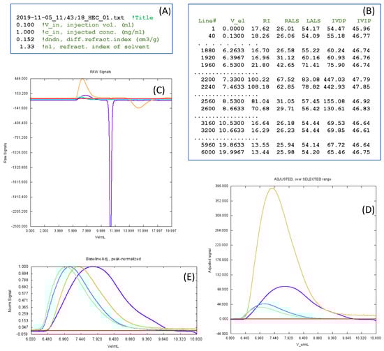
Figure 2.
Some details about the execution of ReadSECRaw 1.0. (A,B) Examples of the two input files: InitData.txt and ReadSECRaw 1.0. Text in green corresponds to labels that have been added here, but do not belong to the real files. In RawSignals.txt, only a few selected lines are shown. (C) Plot of the raw chromatograms corresponding to each detector, with the colors being as follows: RI, violet; LALS, dark green; RALS, light green; IVDP, brown; IVIP, red. Seeing this plot, the user will determine the limits of the range of elution volume, , which contains the peaks. In this example, it was = 6.0–10.8 mL. This way, instrumental artefacts and other features foreign to the macromolecular solute—such as the strong overshoot seen in this case—can be eliminated. Then, the program selects this range, determines the baseline for each detector and calculates them, displays the zero-baseline-corrected chromatograms—plot (D)—and stores the values in the file AdjustedSignalsSelected. Finally, the program constructs and visualizes a plot, (E), of chromatograms that are further normalized to the unit peak height. (C–E) are screenshots of plots displayed during program execution.
4.1.2. SECcal 1.0
The required previous calibration of the detectors is carried out using a standard (i.e., a polymer with a known molecular weight distribution or averages).
SECcal 1.0 first treats the RI data: With the integral (as a discrete sum) of the RI signal, the constant of the RI detector, as defined in Equation (10), is obtained with basis on Equation (22) using the values of and .
The calibration of LS detectors is simpler if the polymer standard has a moderate size, such that the LA approximation applies not only for LALS, but for RALS as well. Equations (27) and (28) could be applied to average over the whole peak to extract the and from the weight-averaged molecular mass, . For either LALS or RALS, the weight averages —required in Equations (26) and (27)—are evaluated from the registers with the weight fractions obtained from the registers using Equations (20) and (21).
Furthermore, if the standard is a nearly monodisperse polymer of molecular weight M, then detector constants and can be determined from Equations (29) and (30), using the values of and , along with the concentration, , of any particular fraction in the chromatogram (concentrations are directly evaluated from the signal according to Equation (21)). The j-th fraction can be that which maximizes the LS signal (i.e., the top of the peak), which maximizes the signal-to-noise ratio.
4.1.3. SECanal 1.0
Once the detector constants have been determined, they are employed in the SECanal 1.0 program to analyze the chromatograms of problem samples. The weight fraction for each slice, , can be directly evaluated from the signals using Equation (20). Having the value of , the concentrations are just = . If the refractive index increment of the sample is unknown, it can be evaluated using the constant of the RI detector by means of Equation (24).
Alternatively, knowing the of the sample, the product can be evaluated from Equation (19), and then proceed to obtain the values as mentioned. If both data points and are available, then the values can be carried out with both procedures to check their concordance.
With the series of values of the LS detectors for each slice, SECanal 1.0 obtains the value of the molecular weight, , both from (Equation (31)) and from (Equation (33)). If the LA approximation holds for both signals, then the two values should coincide, although differences due to instrumental effects may show up. Next, SECanal 1.0 evaluates the intrinsic viscosity, , from the combination of signals from the viscosity detectors and concentration, according to Equation (16) (recall that the viscosity analysis does not require previous calibration).
Then, SECanal 1.0 proceeds, combining all this resulting information in several ways. Combining the vs. values with the vs. values, the resulting series of vs. values provides an essential result in SEC, namely the molecular mass distribution. SECanal 1.0 also provides averages of molecular weight. The weight average is simply
The number fractions are evaluated as
and this enables the determination of other averages, for instance, the number and z averages:
Furthermore, SECanal 1.0 combines the vs. with the vs. . The resulting series of vs. describes the molecular weight dependence of the intrinsic viscosity, which is an essential indicator of the polymer conformation. The intrinsic viscosity of the unfractionated bulk sample is also evaluated. As the contribution of the components of a heterogeneous polymer to the viscosity increments are additive and proportional to concentrations, the bulk intrinsic viscosity is given by
Although these results may be of secondary interest, it could be useful to compare them with those from a separate measurement using conventional viscosimetry, as a way of checking the SEC determinations.
4.1.4. Workflow
Figure 3 presents a workflow indicating in different colours numeric and executable files in the various stages of data analysis. The values indicated as (AdRI)j, (AdLALS)j, and (AdRALS)j are the baseline-adjusted detector signals which are, obviously, those used in the analysis. The diagram includes the optional post-processing with MultyHydFit, as described in a later section.

Figure 3.
Workflow of the computer programs in SECtools. Blue blocks are those of data pre-processing treatment, common to calibration (orange) and analysis (green). Gray blocks are those of post-processing with MultyHydFit.
5. Experimental Results
Here, we present a series of results on real chromatographic experimental data obtained with our chromatograph for several polymer solutions and present the work flow for their analysis using our programs of our SECtools suite, namely, ReadSECRaw 1.0, SECcal 1.0, and SECanal 1.0.
5.1. Instrumentation and Materials
The chromatograph used in our experimental measurements was the Viscotek GPCmax VE-2001 (purchased from Malvern Instruments Ltd., Malvern, UK), coupled to the triple detector array TDA 305, both from Malvern-Viscotek. The detector array includes the following: (a) a differential refractometer measuring the refractive index increment, ; (b) light-scattering detection at two angles—a right angle, RALS, at 90°, and a low angle, LALS, at 7°, with 3 mW laser diode, with the light source being a laser with a wavelength of 670 nm; and (c) a viscosity detector consisting of four capillaries arranged as a differential Wheatstone bridge configuration [24,25]. The setup was equipped with a guard pre-column and one or two size-separating columns, namely, one A4000 column from Malvern-Viscotek and one PL-aquagel-OH-40-8 m column from Agilent Technologies (Santa Clara, CA, USA), serially connected to the first one. The integrated detectors and columns were fully temperature-controlled, with the working temperature being 303 K. The flow rate was 0.7 mL/min in all cases and the injection volume was 100 L.
Instrument control and data acquisition were performed using the Malvern-Viscotek OmniSEC 4.7.0 software. This is a comprehensive software, which additionally carries out a sophisticated protocol for data analysis; however, for the purpose of collecting the raw data to be processed with SECtools programs, OmniSEC 4.7.0 was—in principle—employed just for running the chromatogram and gathering the raw detector signals (mV).
The primary file with the raw experimental data used in our SECtools, named RawData.txt, will first contain the injection data, and , and the refractive index data, and , followed by a tabular list of values of the elution volume, , and the raw signals (mV) of the five detectors, , , , , and , at the j-slices of the chromatogram.
In order to obtain the data for RawData.txt from the OmniSec software, as mentioned above, we wrote an ancillary program, ReadSECRaw 1.0, which can extract the signal data of the TDA 305 module of the Viscotek GPCmax VE-2001. Hopefully, users of other SEC instrumentation will be able to do so for their own interface to SECtools.
5.2. Calibration with Pullulan Standard
The Pullulan standard from Malvern-Viscotek (PolyCAL, referenced PUL-71K, Pul71 in our notation) is practically monodisperse with = 70,768 Da. This was used to calibrate the instrument to obtain the instrument constants , , and (Equations (22), (27), and (32)) by means of SECcal 1.0. The sample concentration was 1 mg/mL.
The chromatograms recorded by OmniSec 4.7.0 were transferred by our ReadSECRaw 1.0 program to file RawData.txt, which is the standard format employed in SECtools. This file was then processed by ReadSECRaw 1.0, which—as indicated above—is in charge of building the input of our calibration program, SECcal 1.0.
Figure 4A shows the resulting multi-detection chromatograms (signals vs. elution volume, ) of the standard Pul71. As can be appreciated, they superimpose perfectly. The polymer elutes over a range of about 2 mL (approximate peak width). An immediate analysis can be made from combinations of detector signals. According to Equations (13) and (14), the LS signals are proportional to the concentration, , of the eluting polymer; therefore, their ratios to are as follows:
The concentration dependence is factored and would depend on and, eventually (if the polymer is large, which is not the case for Pul71) on its size, . Likewise, from Equation (16), is proportional to and the intrinsic viscosity , so that the ratio depends only on .
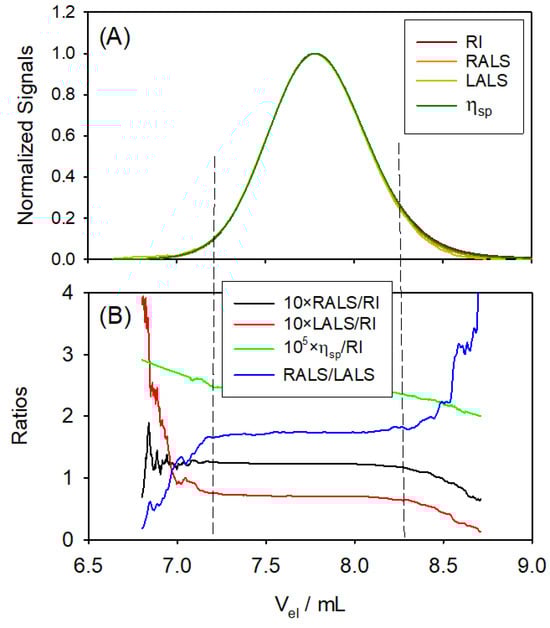
Figure 4.
Experimental results for Pullulan Standard 71 kDa (Pul71). (A) Resulting multi-detection chromatograms (normalized signals vs. elution volume) of the standard Pul71. (B) Signal ratios vs. elution volume. The fluctuations at the tails are a consequence of the very low values of the signals—blurred by detector noises—when concentration is very low.
In Figure 4B, these signal ratios are plotted vs. . The strong fluctuations at the tails of the peak are a simple consequence of the very low values of the signals—which are blurred by detector noises—when the concentration is very low. In the peak region of eluted volume, we note that the ratios are constant, as is obviously the same for all the eluting slices; the polymer is, certainly, monodisperse. Furthermore, the signals corresponding to the various properties show the same trend and reach their maximum peak values at the same , as seen in Figure 4B.
After these inspections, the detector constants are determined using SECcal 1.0. From the given values of , , and , contained in the chromatogram file, SECcal 1.0 uses Equation (22) to give the constant of the RI detector, given in Table 2, and Equation (23) enables the calculation of for every eluting slice. SECcal 1.0 then proceeds to evaluate the LS detector constants. This is performed first from the peak values; the slice that elutes at the peak has the maximum concentration for which g/mL. Then, Equation (29) is used to obtain . With a solute of moderate size, the -dependent term can be ignored, with . For Pullulan with kDa, the radius of gyration should be about 8.9 nm [15], and , which certainly fulfils this condition. Then, the constant of the RALS detector can be determined from Equation (30). SECcal 1.0 also obtains the constants of the LS detectors, obtaining weight averages by integration over the whole chromatogram, thus evaluating from Equation (26) and from Equation (28). The numerical results are presented in Table 2.
Table 2.
Constant detectors for RI, LALS, and RALS, determined by calibration with Pullulan 71 kDa.
5.3. Monodisperse and Paucidisperse Samples
In order to safely check the performance of our data-treatment programs, we proceeded to apply them to experiments carried out with well-characterized samples, containing pure monodisperse polymers or mixtures of them.
In a somehow trivial but illustrative exercise, we consider Pul71 as an unknown sample and process its data files with SECanal 1.0. The results are displayed in Table 3. The excellent agreement with the expected molecular weight was to be expected, as it is the very same sample used for calibration. The merit is, simply, that this confirms the proper functioning of SECanal 1.0. Next, we run three other monodisperse Pullulan samples—namely, Pul48, Pul113, and Pul210 in our notation—purchased from Sigma-Aldrich, Buchs, Switzerland (Fluka, PSS—Pullulan Standard Set (Product number 96351)). The numerical data obtained for the molecular weight are listed in Table 3. The agreement with the nominal values from the standards is most rewarding.
Table 3.
Results for the molecular weight and intrinsic viscosity obtained from our chromatograms, analyzed with our SECtools programs, compared to nominal data and the MHS parameters found in the literature.
Some details of the analysis for sample Pul210 are shown in Figure 5, which shows how the molecular weights for each slice within the peak region, from Equation (31) and from Equation (33), are practically identical, and very close to the nominal one. The molecular weight distribution, shown in the plot of vs. and vs. , presents a sharp peak, as expected, at the nominal M.

Figure 5.
Some results for the Pul210 sample. (A) M determined from the LALS and RALS detection, for each slice over the range of the chromatographic peak. (B) Molecular weight distribution (weight fraction) obtained from the LALS and RALS detectors. As can be appreciated, the molecular weights for each slice within the peak region are practically identical and very close to the nominal one.
Table 3 also contains the SECanal 1.0 results for the intrinsic viscosity, which can be compared with the literature data. Kasaai [31] has reported a Mark–Houwink–Sakurada equation for Pullulan:
As shown in Table 3, our results for of Pullulan standards are in good agreement with the numerical values obtained from Equation (42) with the nominal M of the standards.
A paucidisperse, bicomponent sample—Pul48+805 in our notation—was prepared by mixing two monodisperse Pullulan standards with widely separated molecular weights: 48 kDa and 805 kDa (Fluka, Pullulan Standard Set (Product number 96351), purchased from Sigma-Aldrich, Buchs, Switzerland).
The chromatogram displayed in Figure 6 shows two peaks clearly, the one eluting to lower corresponding to the higher M, and that eluting to higher corresponding to the lower M.

Figure 6.
Chromatograms of the Pul48+805 bimodal sample. (A) Raw signals from all the detectors. (B) Signals adjusted to zero-baseline, and values of the specific viscosity (Equation (15)); all values normalized to unit value for the height of the highest peak. (C) Molecular weights, and , and intrinsic viscosity, , calculated at each slice for each . Plots of log(properties) vs. for this bidisperse sample present two plateaus corresponding to each component peak.
Plots of properties vs. for this bidisperse sample present two regions, each with a plateau region corresponding to the peak of each component. Values of M and of each component can be estimated as the values of the slices in each chromatogram, and the values are included in Table 3. These approximate values are in reasonable agreement with the expected ones, thus showing the qualitative and semi-quantitative good performance of our setup for more complex samples.
5.4. A Polydisperse Sample: 2-Hydroxyethyl Cellulose
Water-soluble cellulose derivatives are appreciably inexpensive polymers that have a number of quite diverse applications, and are particularly suited to be characterized in solution by md-SEC; 2-hydroxyethyl cellulose (2HEC) is a relevant example [32].
Our sample of 2HEC was purchased from Sigma-Aldrich, Buchs, Switzerland (Product number 434964). The procedure for registering the chromatograms and their analysis with our SECtools programs was the same as for the Pullulan samples.
Figure 7 presents some of the results obtained with the SECtools programs. The molecular weight distribution, expressed as weight fraction , shows an interesting aspect of this sample: a somehow bimodal composition, as if it were a mixture of a majority, widely polydisperse component, with a range of M from 103 to 106 Da; and a second component, which appears at mL with a sharper M distribution with a peak at about ∼5.7 (i.e., M∼300 kDa). We also obtained the global properties of the sample; namely, the average molecular weights kDa, kDa, and kDa, with a polydispersity index of PDI∼6. The and results are less reliable than those for , as those averages are more influenced by the shorter and longer polymer chains, respectively, whose M values are affected by instrumental noise. The reason is that they elute at the higher and lower values of , respectively, at which the signal-to-noise ratio of the detectors is important (as evidenced in Figure 7). Furthermore, the global intrinsic viscosity is found to be 115 mL/g.
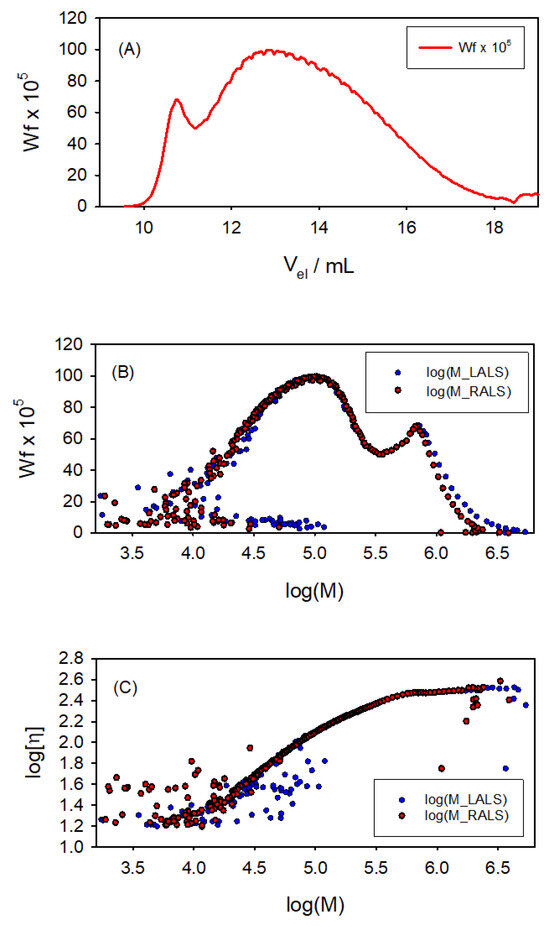
Figure 7.
Results for 2-hydroxyethyl cellulose. (A) Weight fraction along the chromatographic record. (B) Molecular weight distributions from both LALS and RALS detectors. (C) Log–log plot of vs. M, both LALS and RALS. A somehow bimodal composition is appreciated for this sample, as if it were a mixture of a widely polydisperse component, ranging from to Da, and a second component with a peak at about M∼ Da.
The wide molecular weight distribution in this sample also provides its use to illustrate the applicability of the SECtools to obtain structural information, as described in the next section.
6. Structural Determination
In addition to the molecular weight as the primary structural aspect, the dilute-solution properties of macromolecules are an essential source of information on the global structure. The dependence of properties like the intrinsic viscosity, , and the radius of gyration, , on molecular weight, M, depends on the macromolecular chain flexibility; therefore, it is informative about whether the macromolecule is rigid or flexible. For rigid macromolecules, that dependence will be related to the shape, and if flexible, the dependence will be informative about intramolecular and solute–solvent interactions. The possibility of determining the –M relationship from the md-SEC of polydisperse samples is particularly valuable, as shown in the above examples; this is also the case for the –M relationship if the macromolecule is quite large, and even the ratio , where is the hydrodynamic radius obtained from and M [12].
When the solution behavior of the macromolecule can be described by simple models, such as the random-coil (for very long and flexible polymers) or the spherical particle (for some globular proteins), the conformation–property relationships are expressed by simple, usually power-law equations of property vs. molecular weight. However, there are cases for which the theoretical aspects of the model are more complicated, and the extraction of structural parameters from solution property data is more involved. For such cases, we have developed a computer program, MultiHydFit [11,33], which embodies the theory for other models [12], such as short cylindrical particles (short rods and disks) [34] and semi-flexible, Kratky–Porod, worm-like chains (WCs) [35]. The procedure is based on the concept of equivalent radii [11]. The input data are a series of molecular weight values, M, and their corresponding property values, p, where p can be any of the diverse solution properties—including not only and but also including scattering-related and hydrodynamic properties like diffusion and sedimentation. MultiHydFit implements a global fitting procedure for obtaining optimal values of the structural parameters which, in the case of the WC model, are the persistence length P that indicates the degree of stiffness of the chain, its diameter (thickness), d, and the mass per unit of contour length, .
Within the SECtools package, we include an interface that connects the output of SECanal 1.0 to MultiHydFit. The series of , , and eventually —for the many fractions contained in the many slices of the chromatograms—is transferred to a MultiHydFit input file, and then this program obtains the structural parameters. For polymers like polysaccharides, which may present some degree of chain stiffness, the WC is a most appropriate representation. Then, we have used the results for 2-hydroxyethyl cellulose to obtain the WC parameters, obtaining nm, nm, and Da/nm. The P value is not high—it is appreciably smaller than that of other polysaccharides; thus, the cellulose skeleton of the 2HEC derivative is quite flexible. Chain stiffness is the consequence of intramolecular interactions, which, in the case of polyelectrolytes, include electrostatic repulsions. Such is the case for another polysaccharide, alginate, whose stiffness and its corresponding value of P depend on ionic strength. In a previous paper, we used a primitive version of SECtools in an md-SEC study to characterize this dependence [36].
7. Conclusions
In this work, we intended to present the basic aspects of the physical properties of macromolecules in solution and how they are the foundations of the technique of multi-detection size-exclusion chromatography, md-SEC. These fundamental aspects of md-SEC, which are described here with a tutorial purpose, may either be beyond the scope of textbooks, or may somehow have been overlooked in some monographs that are mainly focused on practical aspects and applications. Therefore, the conceptual and mathematical contents of this review may be valuable to beginners in the field and, as such, even for training and teaching purposes.
We implemented the fundamentals in a series of programs for SEC data analysis, contained in our public domain suite SECtools, with open-source codes. Although the SECtools suite of programs basically has the same functionality as other typical programs for GPC analysis—namely, the determination of the molecular weight distribution, molecular weight averages, and the relationship between intrinsic viscosity and the molecular weight—it provides an interface to MultiHydFit (our program for the structural analysis of macromolecules) and is vendor-independent: the input for the data analysis is simply a list of values of the raw (mV) RI, LALS, RALS, IVDP and IVIP detector signals vs. elution volume, . In addition, SECtools has an easy-to-use console dialogue interface and displays graphs during runtime for the visualization of intermediate results, allowing a user to fine-tune the region to be analyzed. We note, also, the valuable possibility of reading, on one hand, the Fortran source code of the programs and, on the other hand, the mathematical basis of the code as described in this paper. The performance of SECtools to extract all the possible information from md-SEC with sufficient accuracy was demonstrated in this article.
Classically, as well as at present, the study of the global structure (i.e., the conformation of macromolecules in solution) was based on measurements of solution properties and the characterization of property–M dependencies and M-dependent property–property relationships. Years ago, this process was performed by carrying out fractional precipitation and, more recently, by preparative chromatography, in order to extract a sufficient number of fractions of sufficiently narrow dispersion, followed by measuring the solution properties of each fraction one after another. With md-SEC, these studies are successfully facilitated. With a single, widely polydisperse sample, a single chromatogram followed by a few steps with appropriate software can produce the different property vs. M data needed for that purpose. As mentioned above, the inclusion of MultiHydFit within SECtools provides an efficient way to obtain structural information. One could affirm that polydispersity was a source of difficulty when used for this purpose years ago; however, at present, by means of md-SEC, it can be regarded as an advantage. With a single, sufficiently polydisperse sample, one can measure the M dependence of properties such as and over a wide range of M values. MultiHydFit can be extended to include other structural models; for instance, rod-like cylinders, disk-like cylinders [33,34] and planar-shaped nanoplatelets [37] for rigid particles, or flexible models for flexible chains with different kinds and extents of branching [38,39,40].
Our description is particularized for a simple md-SEC instrumentation consisting of a concentration detector—namely, a differential refractometer—a dual-angle light-scattering detector, and a capillary-bridge differential viscometer. The extension of the theory and the computational tools to cover md-SEC with multi-angle light-scattering (SEC-MALS) is straightforward; indeed, an array of detectors can be considered in the same way as just a pair. The less-used dynamic light-scattering (SEC-DLS) detector provides an alternative or complementary way to include (like the viscosity detector) a hydrodynamic property, the diffusion coefficient, or the Stokes radius in the information gathered from md-SEC (see, for instance, ref. [41]). Even the more sophisticated detection based on small-angle X-ray scattering (SEC-SAXS) may be a complement to LS to measure the radius of gyration, , and other structural properties of small macromolecules, such as low-molecular-weight polymers, oligomers, proteins, and RNAs [42,43,44,45].
8. Computer Programs
The SECtools suite of computer programs (ReadSECRaw 1.0, SECcal 1.0, and SECanal 1.0) will be freely available, including source codes, detailed user guides, and several examples of input and output files, on our website URL: https://leonardo.inf.um.es/macromol.
Author Contributions
Conceptualization, J.G.d.l.T.; methodology, J.G.d.l.T.; software, J.G.d.l.T. and J.G.H.-C.; validation, J.G.d.l.T. and J.G.H.-C.; formal analysis, J.G.d.l.T., J.G.H.-C. and F.G.D.B.; investigation, F.G.D.B. and M.C.-G.; resources, J.G.d.l.T.; data curation, J.G.H.-C.; writing—original draft preparation, J.G.d.l.T.; writing—review and editing, J.G.H.-C.; visualization, J.G.H.-C. and M.C.-G.; supervision, J.G.d.l.T.; project administration, J.G.H.-C. and M.C.-G.; funding acquisition, J.G.H.-C. and M.C.-G. All authors have read and agreed to the published version of the manuscript.
Funding
The authors greatly appreciate the financial support provided by grant TED2021-130334B-I00 funded by MICIU/AEI/10.13039/501100011033/ and by the European Union “NextGenerationEU/PRTR”. Funding was also provided through the call for Grants for Projects for the Generation of New Scientific Leadership “Young Leaders in Research” (22010/JLI/22) included in the Regional Program for the Promotion of Scientific and Technical Research (Action Plan 2022) of the Seneca Foundation of Science and Technology of Murcia (Spain). The publication is part of the grant RYC2021-034184-I funded by MCIN/AEI/10.13039/501100011033 and by the European Union “NextGenerationEU/PRTR”. This work has been partially supported by grants with the refs. TED2021-130389B-C21, PID2020-113081RB-I00, and PID2023-150761OB-C21, funded by MCIN/AEI/ 10.13039/501100011033 and by EU “Next Generation”, and part of the grant ref. 22129-PI-22 funded by the research support program of the Seneca Foundation of Science and Technology of Murcia (Spain).
Institutional Review Board Statement
Not applicable.
Data Availability Statement
Data are contained within the article.
Conflicts of Interest
The authors declare no conflicts of interest.
References
- Sun, S.F. Physical Chemistry of Macromolecules, 2nd ed.; John Wiley and Sons: Hoboken, NJ, USA, 2004. [Google Scholar]
- Hiemenz, P.C.; Lodge, T.P. Polymer Chemistry, 2nd ed.; CRC Press: Boca Raton, FL, USA, 2007. [Google Scholar]
- Snyder, L.R.; Kirkland, J.J. Introduction to Modern Liquid Chromatography; Wiley: New York, NY, USA, 1974. [Google Scholar]
- Serdyuk, I.N.; Zaccai, N.R.; Zaccai, J. Methods in Molecular Biophysics. Structure, Dynamics, Function; Cambridge University Press: New York, NY, USA, 2007. [Google Scholar]
- Striegel, A.M.; Kirkland, J.J.; Yau, W.W.; Bly, D.D. (Eds.) Modern Size-Exclusion Chromatography, 2nd ed.; Wiley: New York, NY, USA, 2009. [Google Scholar]
- Wu, C.S. (Ed.) Handbook of Size Exclusion Chromatography and Related Techniques, 2nd ed.; Dekker: New York, NY, USA, 2004. [Google Scholar]
- Grubisic, Z.; Rempp, P.; Benoit, H. A universal calibration for gel permeation chromatography. J. Polym. Sci. Part C Polym. Lett. 1967, 5, 753–759. [Google Scholar] [CrossRef]
- Horta, A.; Saiz, E.; Barrales-Rienda, J.M.; Galera Gomez, P.A. Direct estimation of the true Mark-Houwink-Sakurada parameters from gel permeation chromatography, intrinsic viscosity and one average of molecular weight. Polymer 1986, 27, 139–146. [Google Scholar] [CrossRef]
- Einstein, A. A new determination of molecular dimensions. Ann. Phys. 1906, 19, 289–306. [Google Scholar] [CrossRef]
- Flory, P.J.; Fox, T.G. Treatment of intrinsic viscosity. J. Am. Chem. Soc. 1951, 73, 1904–1908. [Google Scholar] [CrossRef]
- Ortega, A.; García de la Torre, J. Equivalent radii and ratios of radii from solution properties as indicators of macromolecular conformation, shape, and flexibility. Biomacromolecules 2007, 8, 2464–2475. [Google Scholar] [CrossRef]
- García de la Torre, J.; Hernández Cifre, J.G. Hydrodynamic properties of biomacromolecules and macromolecular complexes: Concepts and methods. A tutorial mini-review. J. Mol. Biol. 2020, 432, 2930–2948. [Google Scholar] [CrossRef]
- Rubinstein, M.; Colby, R.H. Polymer Physics; Oxford University Press: New York, NY, USA, 2003. [Google Scholar]
- Kröger, M. Models for Polymeric and Anisotropic Liquids; Springer: Berlin/Heidelberg, Germany, 2005. [Google Scholar]
- Fishman, M.L.; Damert, W.C.; Phillips, J.G.; Barford, R.A. Evaluation of root-mean-square radius of gyration as a parameter for universal calibration of polysaccharides. Carbohydr. Res. 1987, 160, 215–225. [Google Scholar] [CrossRef]
- Kashiwagi, K.; Norisuye, T.; Fujita, H. Triple helix of schizophyllum commune polysaccharide in dilute solution. 4. light scattering and viscosity in dilute aqueous solution. Macromolecules 1981, 14, 1220–1225. [Google Scholar] [CrossRef]
- Ioan, C.E.; Aberle, T.; Burchard, W. Structure properties of dextran. 2. Dilute solution. Macromolecules 2000, 33, 5730–5739. [Google Scholar] [CrossRef]
- Linegar, K.L.; Adeniran, A.E.; Kostko, A.F.; Anisimov, M.A. Hydrodynamic radius of polyethylene glycol in solution obtained by dynamic light scattering. Colloid J. 2010, 72, 279–281. [Google Scholar] [CrossRef]
- Devannand, K.; Selser, J.C. Asymptotic behavior and long-range interactions in aqueous solutions of poly(ethylene oxide). Macromolecules 1991, 24, 5943–5947. [Google Scholar] [CrossRef]
- Krigbaum, W.R.; Kuegler, F.R. Molecular conformation of egg-white lysozyme and bovine α-lactalbumin in solution. Biochemistry 1970, 9, 1216–1223. [Google Scholar] [CrossRef] [PubMed]
- Wilhelm, P.; Pilz, I.; Palm, W.; Bauer, K. Small-angle X-ray studies of a human immunoglobulin M. Eur. J. Biochem. 1978, 84, 457–463. [Google Scholar] [CrossRef]
- Godfrey, J.E. The flexibility of low molecular weight double-stranded DNA as a function of length: (I). Isolation and physical characterization of seven fractions. Biophys. Chem. 1976, 5, 285–299. [Google Scholar] [CrossRef]
- Müller, J.J.; Zalkova, T.N.; Ziwer, D.; Misselwitz, R.; Gast, K.; Serdyuk, I.N.; Welfle, H.; Damaschun, G. Comparison of the structure of ribosomal 5S RNA from E. coli and from rat liver using X-ray scattering and dynamic light scattering. Eur. Biophys. J. 1986, 13, 301–307. [Google Scholar] [CrossRef]
- Haney, M.A. The differential viscometer. I. A new approach to the measurement of specific viscosity of polymer solutions. J. Appl. Polym. Sci. 1985, 30, 3023–3026. [Google Scholar] [CrossRef]
- Haney, M.A. The differential viscometer. II. On-line viscosity detector for size-exclusion chromatography. J. Appl. Polym. Sci. 1985, 30, 3037–3049. [Google Scholar] [CrossRef]
- Dutta, P.K.; Hammons, K.; Willibey, B.; Haney, M.A. Analysis of protein denaturation by high-performance continuous differential viscometry. J. Chromatog. 1991, 536, 113–121. [Google Scholar] [CrossRef]
- Harding, S.E. The intrinsic viscosity of biological macromolecules. Progress in measurement, interpretation and application to structure in dilute solution. Prog. Biophys. Mol. Biol. 1997, 68, 207–262. [Google Scholar] [CrossRef]
- Solomon, O.F.; Ciuta, I.Z. Détermination de la viscosité intrinsèque de solutions de polymères par une simple détermination de la viscosité. J. Appl. Polym. Sci. 1962, 6, 683–686. [Google Scholar] [CrossRef]
- Solomon, O.F.; Gotesman, B.S. Calculation of viscosity number from a single measurement. Makromol. Chem. 1967, 104, 177–184. [Google Scholar] [CrossRef]
- Pamies, R.; Hernández Cifre, J.G.; López Martínez, M.C.; García de la Torre, J. Determination of intrinsic viscosities of macromolecules and nanoparticles. Comparison of single-point and dilution procedures. Colloid Polym. Sci. 2008, 286, 1223–1231. [Google Scholar] [CrossRef]
- Kasaai, M.R. Intrinsic viscosity—Molecular weight relationship and hydrodynamic volume for pullulan. J. Appl. Polym. Sci. 2006, 100, 4325–4332. [Google Scholar] [CrossRef]
- Marcelo, G.; Saiz, E.; Tarazona, M.P. Determination of molecular parameters of hydroxyethyl and hydroxypropyl celluloses by chromatography with dual detection. J. Chromatogr. A 2007, 1165, 45–51. [Google Scholar] [CrossRef]
- Ortega, A.; Amorós, D.; García de la Torre, J. Global fit and structure optimization of flexible and rigid macromolecules and nanoparticles from analytical ultracentrifugation and other dilute solution properties. Methods 2011, 54, 115–123. [Google Scholar] [CrossRef]
- Ortega, A.; García de la Torre, J. Hydrodynamic properties of rodlike and disklike particles in dilute solution. J. Chem. Phys. 2003, 119, 9914–9919. [Google Scholar] [CrossRef]
- Amorós, D.; Ortega, A.; Harding, S.E.; García de la Torre, J. Multi-scale calculation and global-fit analysis of hydrodynamic properties of biological macromolecules: Determination of the overall conformation of antibody IgG molecules. Eur. Biophys. J. 2010, 39, 361–370. [Google Scholar] [CrossRef]
- Díaz Baños, F.G.; Díez, A.; Hernández Cifre, J.G.; López Martínez, M.C.; Ortega, A.; García de la Torre, J. Influence of ionic strength on the flexibility of alginate studied by size exclusion chromatography. Carbohydr. Polym. 2014, 102, 223–230. [Google Scholar] [CrossRef]
- Hernández Cifre, J.G.; Rodríguez-Schmidt, R.; Almagro-Gómez, C.M.; García de la Torre, J. Calculation of the friction, diffusion and sedimentation coefficients of nanoplatelets of arbitrary shape. Polymer 2022, 262, 125467. [Google Scholar] [CrossRef]
- Freire, J.J. Conformational properties of branched polymers: Theory and simulations. In Advances in Polymer Science. Branched Polymers II; Roovers, J., Ed.; Springer: Berlin/Heidelberg, Germany, 1999; pp. 35–112. [Google Scholar]
- Del Río Echenique, G.; Rodríguez Schmidt, R.; Freire, J.J.; Hernández Cifre, J.G.; García de la Torre, J. A multiscale scheme for the simulation of conformational and solution properties of different dendrimer molecules. J. Am. Chem. Soc. 2009, 131, 8548–8556. [Google Scholar] [CrossRef]
- Rodríiguez Schmidt, R.; Hernández Cifre, J.G.; García de la Torre, J. Multi-scale simulation of hyperbranched polymers. Polymers 2015, 7, 610–628. [Google Scholar] [CrossRef]
- Deng, J.Z.; Rustandi, R.R.; Swartz, A.; Shieh, Y.; Baker, J.B.; Vlasak, J.; Wang, S.; Loughney, J.W. SEC coupled with in-line multiple detectors for the characterization of an oncolytic Coxsackievirus. Mol. Ther. Oncolytics 2022, 24, 139–147. [Google Scholar] [CrossRef] [PubMed]
- Brookes, E.; Vachette, P.; Rocco, M.; Pérez, J. US-SOMO HPLC-SAXS module: Dealing with capillary fouling and extraction of pure component patterns from poorly resolved SEC-SAXS data. J. Appl. Cryst. 2016, 49, 1827–1841. [Google Scholar] [CrossRef] [PubMed]
- Bucciarelli, S.; Midtgaard, S.R.; Pedersen, M.N.; Skou, S.; Arleth, L.; Vestergaard, B. Size-exclusion chromatography small-angle X-ray scattering of water soluble proteins on a laboratory instrument. J. Appl. Cryst. 2018, 51, 1623–1632. [Google Scholar] [CrossRef] [PubMed]
- Graewert, M.A.; Vela, S.D.; Gräwert, T.W.; Molodenskiy, D.S.; Blanchet, C.E.; Svergun, D.I.; Jeffries, C.M. Adding size exclusion chromatography (SEC) and light scattering (LS) devices to obtain high-quality small angle X-ray scattering (SAXS) data. Crystals 2020, 10, 975. [Google Scholar] [CrossRef]
- Matsui, T.; Rajkovic, I.; Mooers, B.H.; Liu, P.; Weiss, T.M. Adaptable SEC-SAXS data collection for higher quality structure analysis in solution. Protein Sci. 2024, 33, e4946. [Google Scholar] [CrossRef]
Disclaimer/Publisher’s Note: The statements, opinions and data contained in all publications are solely those of the individual author(s) and contributor(s) and not of MDPI and/or the editor(s). MDPI and/or the editor(s) disclaim responsibility for any injury to people or property resulting from any ideas, methods, instructions or products referred to in the content. |
© 2025 by the authors. Licensee MDPI, Basel, Switzerland. This article is an open access article distributed under the terms and conditions of the Creative Commons Attribution (CC BY) license (https://creativecommons.org/licenses/by/4.0/).