3.1.1. Density
We start the analysis of the model PNCs with the calculation of the mass monomer density profile of the polymer (PE) chains as a function of the distance from the graphene sheet. Average density profiles, which have been calculated for the center of mass of the monomers,
ρ(
r), are presented in
Figure 2a,d for all four systems. In
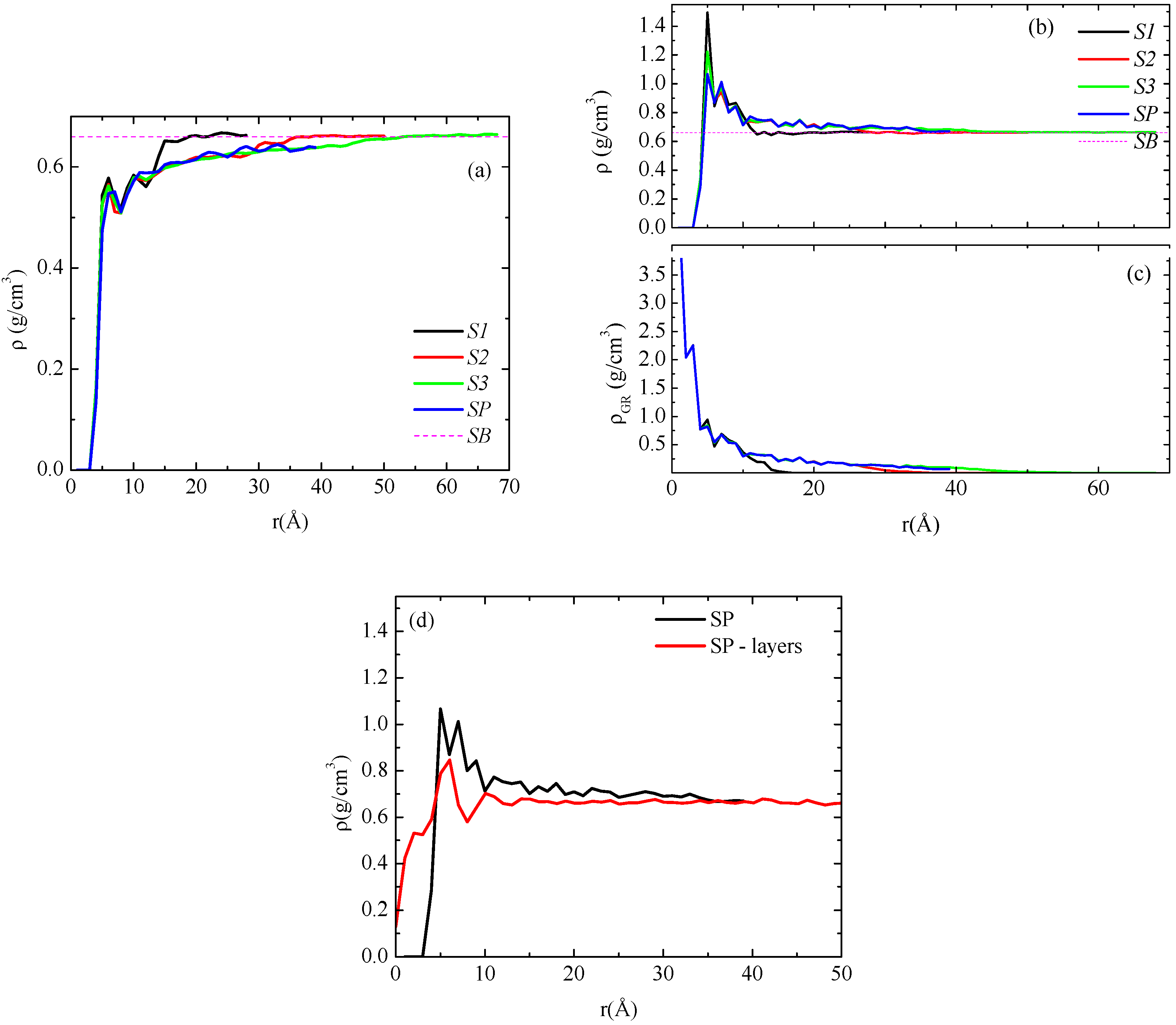
Figure 2a, the polymer mass at each spherical shell has been divided with the total volume of the shell, which for the inner shells contains a number of graphene atoms as well, whereas the outer shells contain only polymer atoms. For this reason in
Figure 2a PE mass density values at short distances are smaller than the corresponding bulk density value, while for longer distances bulk density is attained from the three systems with the finite graphene sheets. For the system with the infinite size graphene, monomer density approaches, but do not reach, the corresponding bulk value since graphene mass exists in all spherical shells. In all four systems the density of PE close to the sheet is almost the same and unaffected by the size of the sheet. Αway from the graphene layer, all curves reach/approach the bulk density value, though at different distances, as a result of the graphene sheet dimensions.
Figure 2.
(a) Mass monomer density profiles of polyethylene as a function of r (distance from the center of the graphene layer) for the five systems studied here; (b) Density profiles of polyethylene chains excluding the volume occupied by graphene; (c) Mass density profiles of graphene layer as a function of r; (d) Density profile of polyethylene chains for the periodic graphene layer analyzed via spherical shells and parallel slabs.
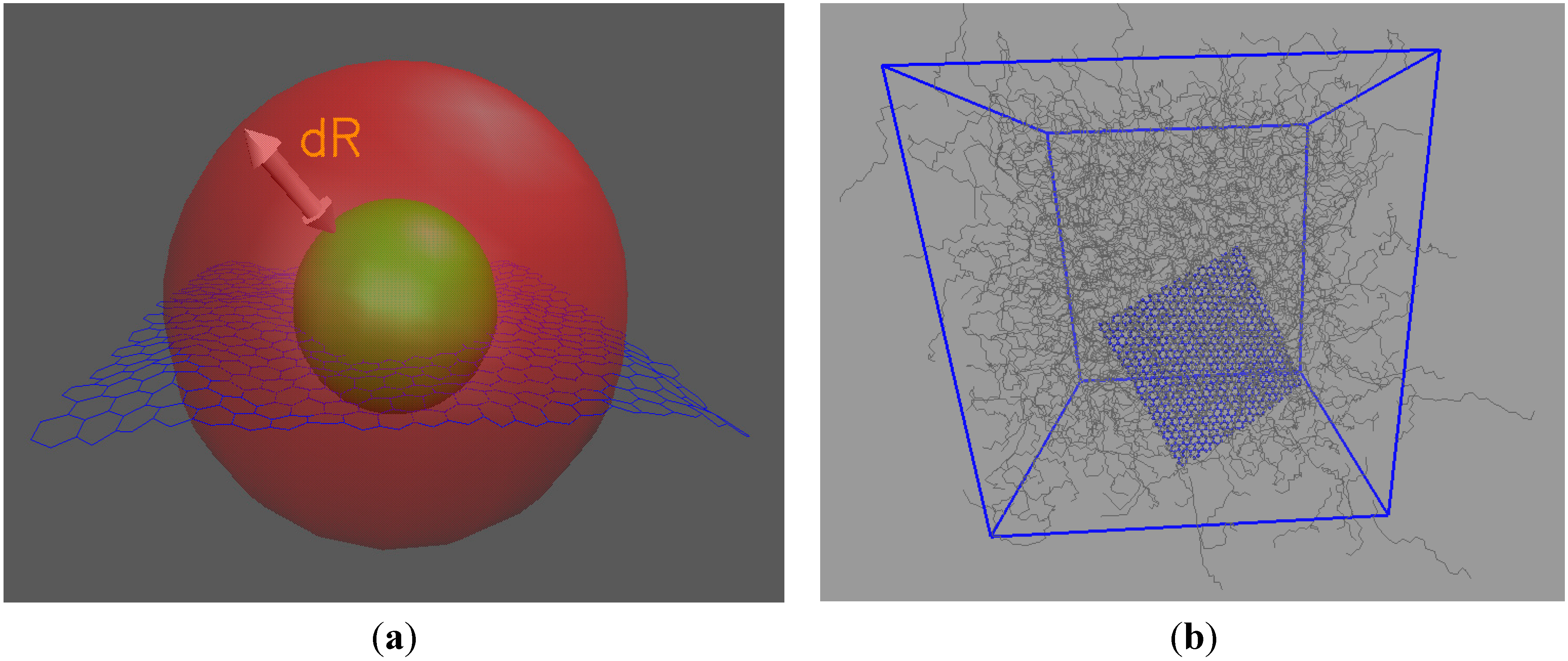
In the next stage PE monomer density profiles are calculated dividing the polymer mass with a portion of the spherical shell volume that corresponds to this mass. For this purpose we have performed a rough estimation for the volume that graphene atoms occupy in each spherical shell and subtracted it from the total volume of the shell. This has been performed as mentioned in the previous section, through the following procedure: First, a sphere with a radius equal to a distance of 3.47 Å, which corresponds to the excluded volume between an atom in the graphene sheet and the polymer, is defined and the number of graphene atoms in this sphere is counted. No polymer atoms are included in this volume. Through these values the average effective volume occupied by each graphene atom in the graphene sheet is calculated. Second, the number of graphene atoms in any spherical shell is computed. Then, we calculate their effective volume within each spherical shell and subtract it from the volume of the whole shell. Finally, polymer mass is divided with the remaining volume which corresponds to the polymer atoms. In
Figure 2c the density of the amount of the graphene in each spherical shell is presented for all systems studied here. We observe that these curves attain the same values up to a specific distance, defined from the size of the sheet, beyond which no more graphene atoms are included in the spherical shell.
Chain density profiles, derived with the above procedure, for all model systems are shown in
Figure 2b. All systems exhibit the same behavior: a peak of rather similar height (larger than the bulk value) is observed for all four systems at a distance/radius of about 0.5 nm, which denotes the attraction of the polymer from the graphene at short distances, while at longer distances the bulk density is attained.
As mentioned in
Section 2 one issue related to the analysis method using spherical cells, is that this might not be the natural choice for systems with the infinite-periodic graphene sheet. For the latter the analysis in parallel slabs seems to be a more appropriate choice [
18]. In
Figure 2d we compare the density profiles of the polymer chains for this system (SP) and the two different analysis methods;
i.e., using spherical shells and parallel slabs. As we can see there are slight differences for the ρ(
r) data between the two methods in the region of 1–2 nm from the graphene sheet. Note finally that for the case of the parallel slabs the zero is defined on the position of the center of the graphene sheet, therefore due to thermal undulations of graphene it is probable to have polymer mass at zero distance.
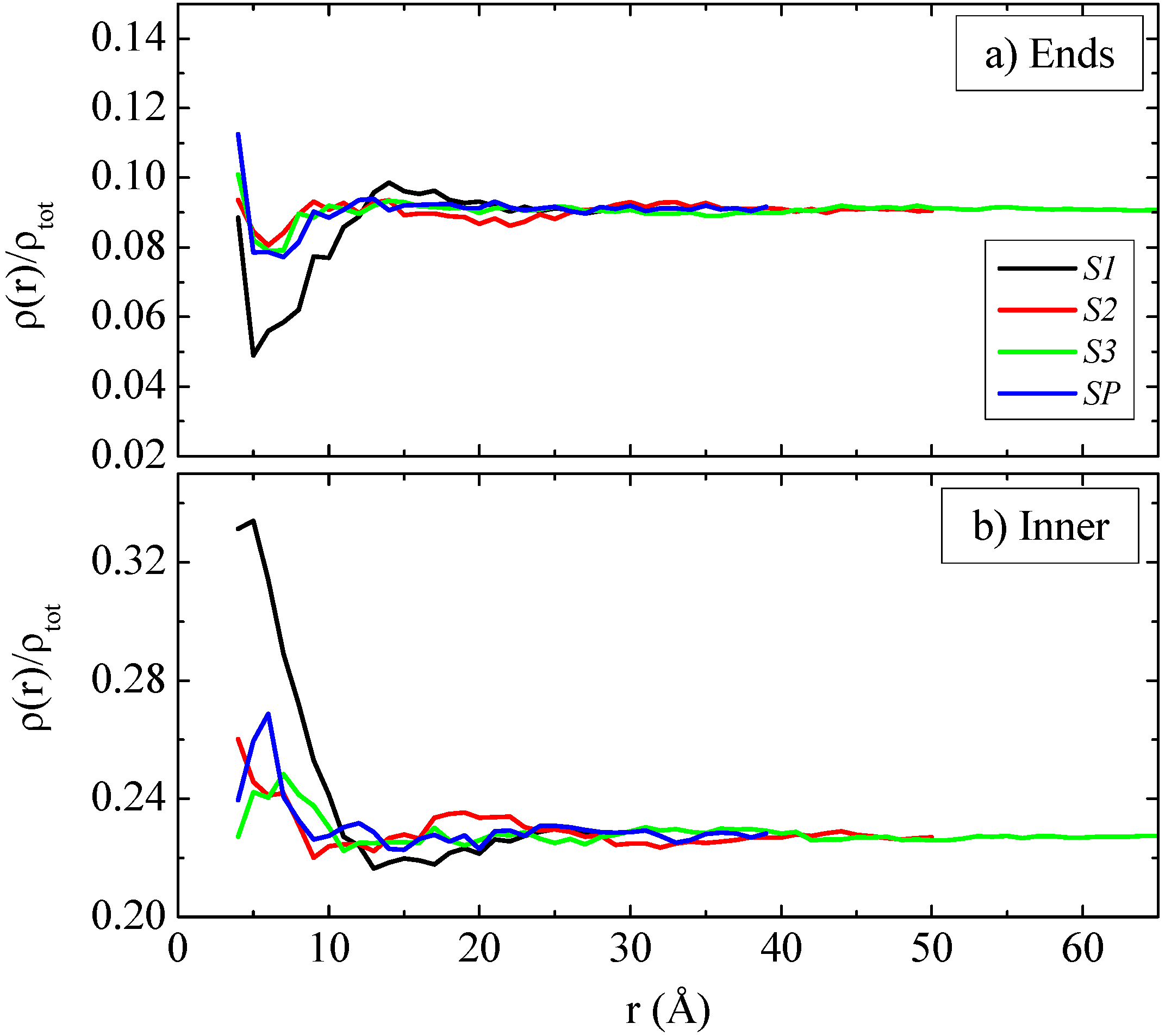
In the following we analyze the distribution of ends and inner parts of the polymer chains at the PE/graphene interface. The preference of the chain ends to stay close to the surface, compared to the rest of the monomers, has been reported in previous studies of polymer/surface interfaces and it is primary of entropic origin [
17]. We have also observed this behavior in our previous studies at the polymer/graphene interface of polymer thin films confined between two “infinite” (periodic) graphene sheets, as well as at polymer/vacuum interface [
20,
21,
26]. A similar analysis has been performed in our current systems for both the end and the inner monomers. It is interesting to observe the effect of the motion of the sheet, the range of fluctuations and the different size on this tendency. In
Figure 3a,b the density profiles based on the monomer center of mass for the end and the inner monomers are presented for all systems, respectively. The “end part” concerns only two monomers, the first and the last one, while the “inner part” is defined as the monomers of the chain in the interval
, where
N is the total number of monomers per chain. Following such a convention some monomers on the left and on the right side of the central part of the chain do not participate in the analysis; thus avoiding any contribution of the chain end effects in the analysis of the inner segments and vise-versa. For the infinite layer the preference of the ends for the interface is comparable to the one observed before for a PE/graphene system with a frozen graphene layer [
17,
21];
i.e., thermal fluctuations of a very large (“infinite”) graphene sheet are not very important for the overall chain arrangement at the PE/graphene interface.
Qualitatively different is the case for the systems with the finite graphene sheets. Data presented in
Figure 3a for the two smaller sheets show that although an amount of end monomers are concentrated close to the graphene flake they do not exceed the highest density. In more details, for the S1 system the accumulation of end monomers in the bulk region is higher than the one at the interface, while for the S2 system the density of the end monomers at the interface increases and is almost equal to that in the bulk region. For the largest sheet (S3 system) there is a small increase of the end monomers’ density close to the graphene layer, compared to the two smaller systems (S1, S2), which roughly speaking indicates a tendency of the end monomers to be accumulated at the interface. The preference of the end monomers for the interface becomes clear only in the case of “infinite” graphene layer (SP). The density profiles for the inner monomers, shown in
Figure 3b, have a complementary to the end monomers behavior, as expected. This is a combinatory effect of the size, the mobility and the fluctuations of the sheet and as it will be discussed in a following section,
i.e., the smaller the sheet the higher its mobility while the smaller its fluctuations. In addition, for the graphene sheets of finite size considerable system size effects exist, which are more pronounced for the smaller sizes.
Figure 3.
Mass monomer density profiles as a function of R (distance from the center of the graphene layer) based on (a) chain ends and (b) inner monomers of the polymer chain for the polymer/graphene nanocomposite systems.
Figure 3.
Mass monomer density profiles as a function of R (distance from the center of the graphene layer) based on (a) chain ends and (b) inner monomers of the polymer chain for the polymer/graphene nanocomposite systems.
3.1.2. Conformational Properties
We start the analysis of the chain conformations by calculating the average chain end-to-end distance,
, and the radius of gyration,
. An important question concerns whether chain swelling occurs due to chain adsorption at the polymer/graphene interface. In
Table 2 we report data concerning the end-to-end distance of the polymer chains as a function of distance from the graphene sheets. As we can see chain dimensions are rather similar at all distances (and same to the bulk values) but the very first layer where a slight increase of the
Ree and
Rg are observed. However, the latter values are within the error bars.
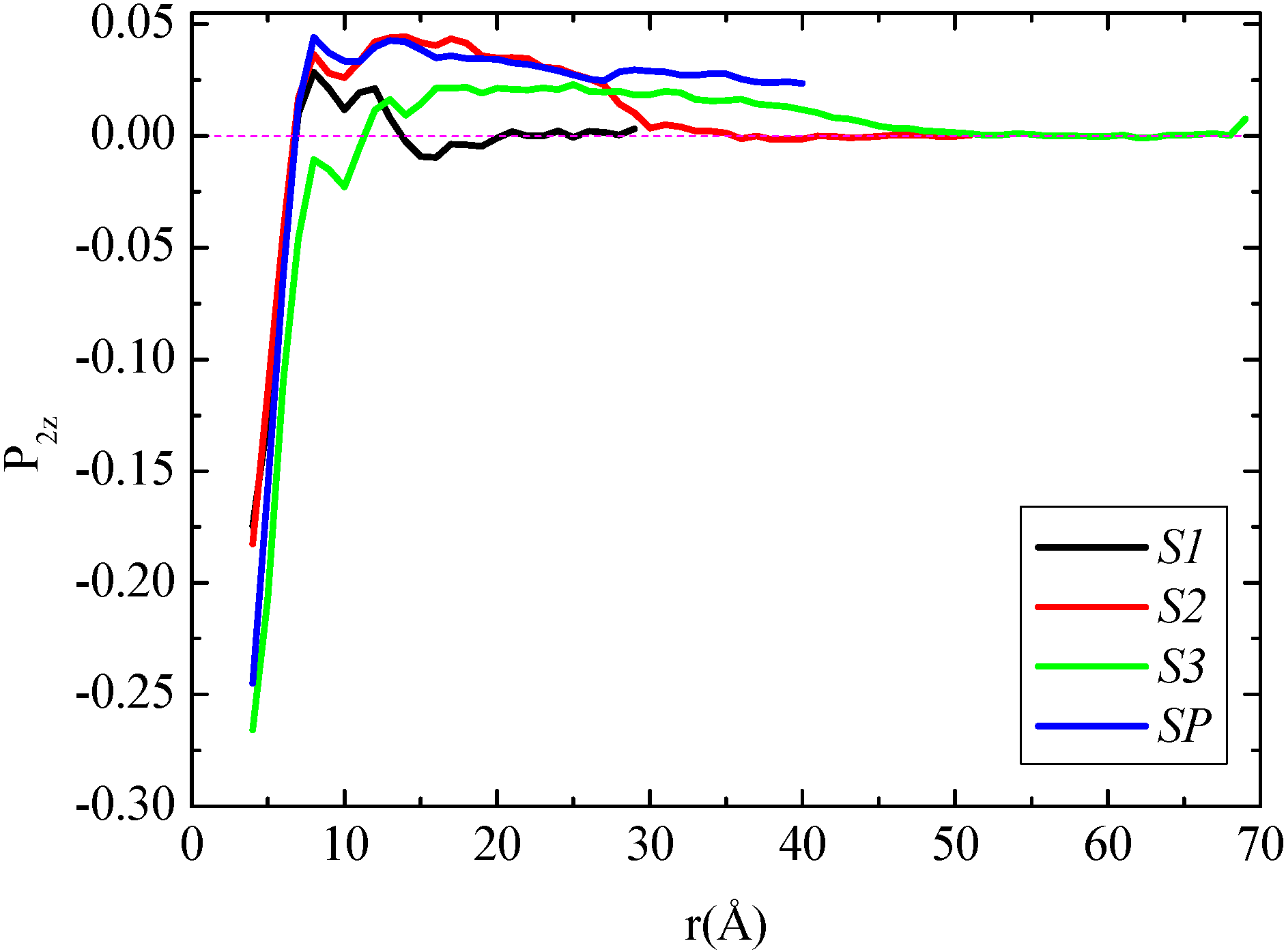
In the following we examine the orientation of the polymer chains close to the graphene layer in the segmental level through the
v1−3 vector which connects two non-consecutive carbon atoms. In more detail, the second rank bond order parameter [
27,
28] defined as
is calculated.
P2(cosθ) limiting values of
−0.5, 0.0, and 1.0 correspond to perfectly parallel, random, and perpendicular vector orientations relative to the graphene layer, respectively. In the above formula θ is the angle between the vector, which is defined along the molecule (here the
v1−3 one) and the radial distance from the center of graphene. The bond order parameter of
v1−3 for all four systems is depicted in
Figure 4. In all cases there is an obvious tendency of the segments of the polymer chain for an almost parallel to the graphene layer orientation at short distances which is gradually randomized with the distance. However, there is a systematic increase of the order of the PE segments closest to the graphene layer with the increase of the size of the layers; the minimum values are about −0.17 for the two smaller sheets, whereas the value for the system with the largest sheet (S3) is about −0.25 very similar to that of the infinite sheet.
Table 2.
Average chain end-to-end distance,
, and radius of gyration,
for chains belonging in different adsorption layers, R. Corresponding bulk values: Ree = 17.20 Å, Rg = 6.15 Å. Error bars are 3%–5% of the actual values based on block averaging techniques.
Table 2.
Average chain end-to-end distance,
, and radius of gyration,
for chains belonging in different adsorption layers, R. Corresponding bulk values: Ree = 17.20 Å, Rg = 6.15 Å. Error bars are 3%–5% of the actual values based on block averaging techniques.
| R (Å) | Ree (Å) | Rg(Å) |
|---|
| S1 | S2 | S3 | SP | S1 | S2 | S3 | SP |
|---|
| 0–6 | 17.30 | 17.46 | 17.48 | 17.48 | 6.44 | 6.55 | 6.51 | 6.46 |
| 6–10 | 17.28 | 17.41 | 17.44 | 17.46 | 6.32 | 6.54 | 6.50 | 6.45 |
| 10–20 | 17.24 | 17.33 | 17.36 | 17.41 | 6.28 | 6.31 | 6.36 | 6.35 |
| 20–30 | 17.23 | 17.28 | 17.32 | 17.37 | 6.21 | 6.24 | 6.28 | 6.27 |
| 30–40 | 17.22 | 17.25 | 17.30 | 17.35 | 6.18 | 6.22 | 6.23 | 6.26 |
| 40–50 | - | 17.24 | 17.27 | 17.33 | - | 6.20 | 6.23 | 6.23 |
| 50–60 | - | 17.24 | 17.25 | 17.31 | - | 6.18 | 6.21 | 6.19 |
| 60–70 | - | - | 17.25 | - | - | - | 6.20 | - |
| 70–80 | - | - | 17.25 | - | - | - | 6.19 | - |
Figure 4.
Second rank bond order parameter P2(cosθ) of polyethylene for v1−3 vector as a function of R distance (distance from the center of the graphene layer) for all polymer/graphene nanocomposite systems studied here.
Figure 4.
Second rank bond order parameter P2(cosθ) of polyethylene for v1−3 vector as a function of R distance (distance from the center of the graphene layer) for all polymer/graphene nanocomposite systems studied here.
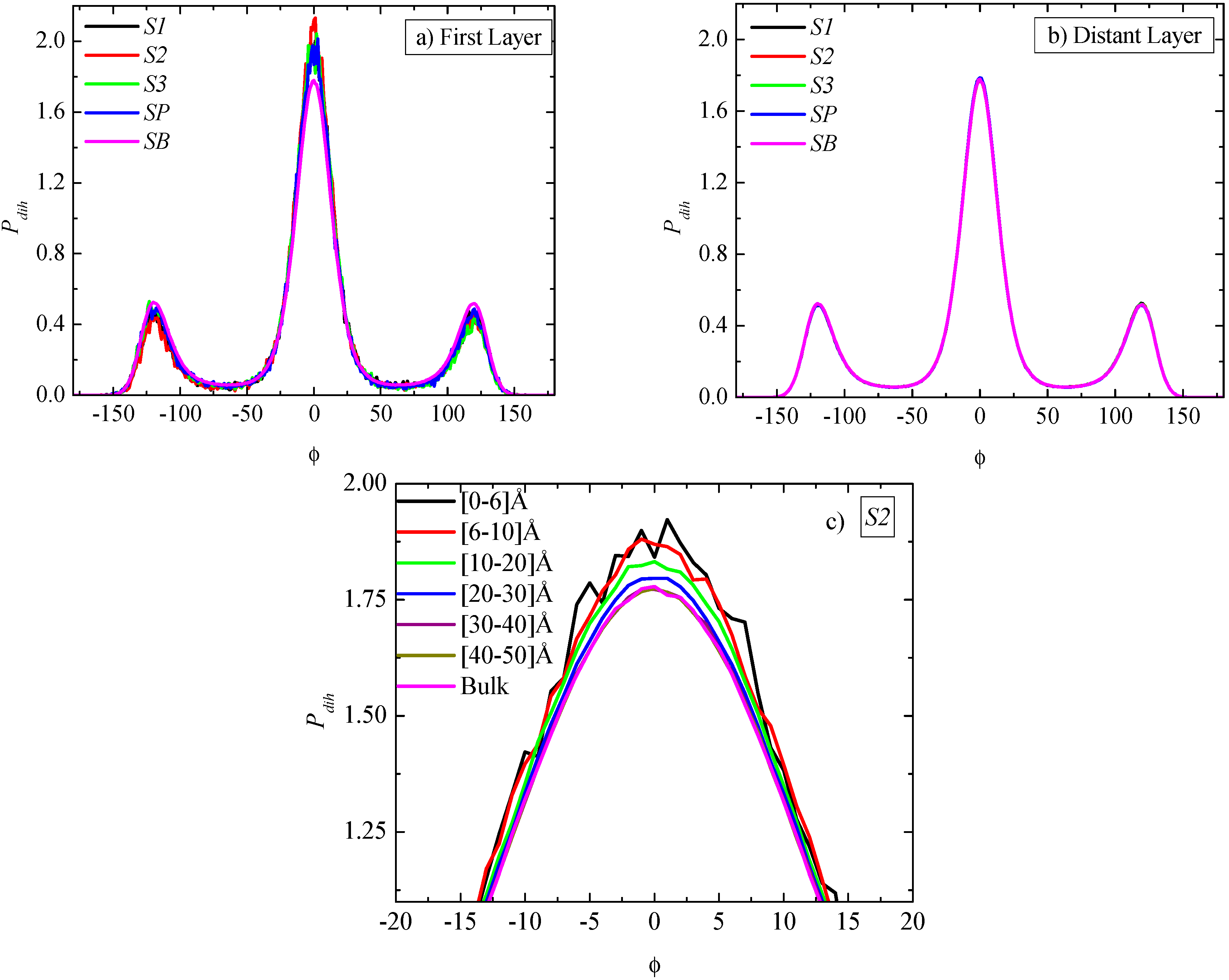
A further analysis of the PE chain conformations is based on the calculation of the distribution of the torsional (dihedral) angles,
Pdih, in different distances from graphene. This is of particular importance since for PE the distribution of its (backbone) dihedral angle is critical for the determination of its overall chain conformation (e.g., radius of gyration and characteristic ratio). In the analysis performed here all torsional angles with values between −60
° and +60
°, are defined as “trans”, whereas outside this interval angles are considered as “gauche+” or “gauche−”. Our results which are depicted in
Figure 5a–c indicate clear spatial heterogeneous dihedral angle distribution, for all PNCs.
Figure 5a contains a comparison of the distribution of the torsional angles in the (spherical) first adsorption layer (
i.e., from 0 to 6 Å) for the four systems together with the corresponding bulk system. A non-negligible enhancement of the trans states with a consequent reduction of the gauche ones is observed for all systems compared to the bulk case. This observation reflects the more ordered PE chains close to the graphene sheet, something which has been reported previously as well, for thin polymer films supported by graphene or graphite [
17,
18]. Enhancement of “trans” population would be expected to affect the cystallinity of PE chains as well as the mechanical properties of the hybrid PNC system. This will be studied in a forthcoming work. Moreover no differentiation in the torsional angle distributions among the various sizes of graphene sheets is detected. The corresponding information for the most distant adsorption layer (
i.e., bulk region) is presented in
Figure 5b, where the curves are completely identical to each other and to the corresponding bulk one.
Figure 5.
Torsional angles distribution as a function of R distance (distance from the center of the graphene layer). (a) Data for the first adsorption layer (R = 0.6 nm) for all systems; (b) Data for the last adsorption layer (distant layer) (R = LBOX/2) for all systems; (c) Magnification for all spherical shells of the (S2) system. In all cases the corresponding bulk curve is included.
Furthermore, if we compare
Pdih as a function of radial distance from the center of the graphene sheet, the enhancement of “trans” states remains, presenting a small but gradual decrease compared to the first adsorption layer, up to a different distance depending on the system. Beyond a specific distance for each system the rest of the curves coincide with those of
Figure 5b. The enhancement of “trans” states for dihedral angles of the S2 system, and for the various regimes studied here, is presented in
Figure 5c, where it is clear that the curves are distance dependent, despite the rather noisy data due to the small size of each regime. Overall, the distance above which all
Pdih’s become similar to the bulk
Pdih defines the width of the interphase for the particular property and the way that it is affected by each graphene sheet. The effect can be thought as a combination of the differentiations among the sheets (
i.e., size, mobility, fluctuations), which will be analyzed in detail in a following section.
Based on the above discussion of the spatial chain structural-conformational heterogeneities, a rough estimation of the distance beyond which the bulk behavior of the hybrid PNC system, is attained can be given as: (~r ≤ 10 Å), for the smallest graphene sheet, (S1), extended to larger values (~r ≤ 30 Å) for the S2 system and even further (~r ≤ 40 Å) for the S3 system, while for the infinite graphene layer (SP) system size limitations do not allow the prediction of a specific value for the distance beyond which the bulk behavior is attained.
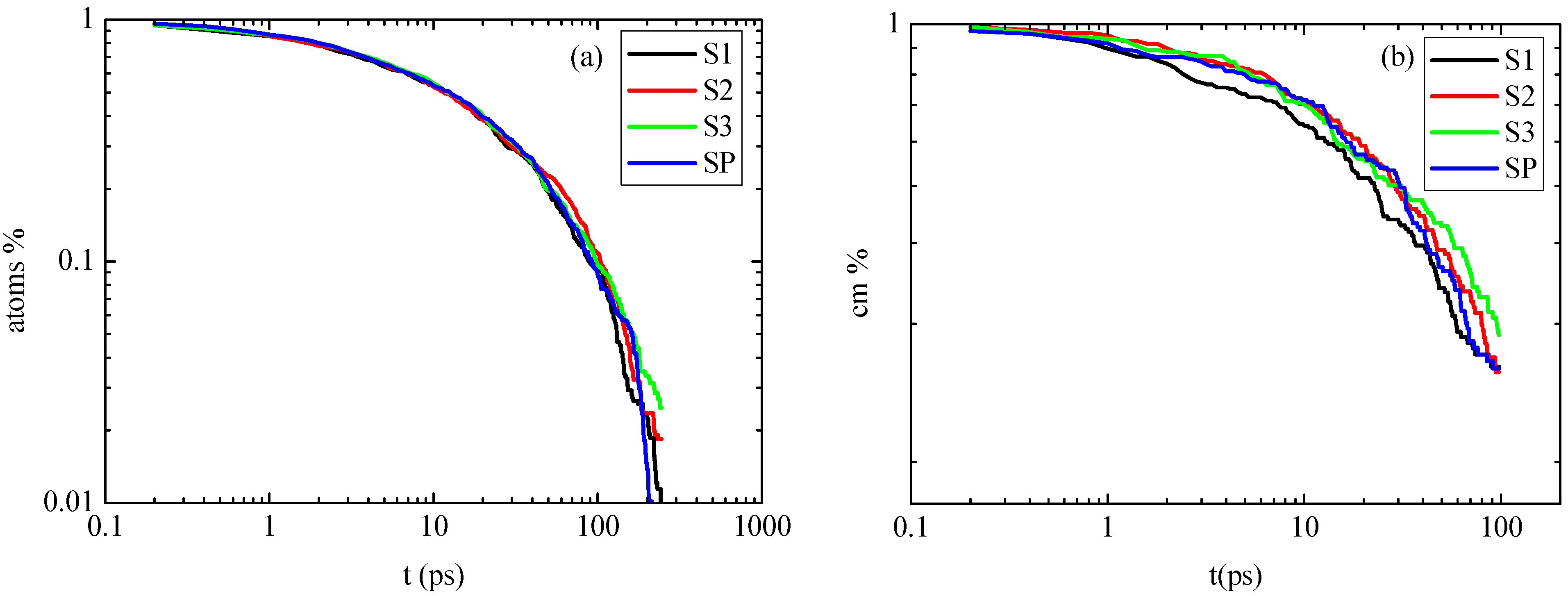
3.1.3. Dynamics
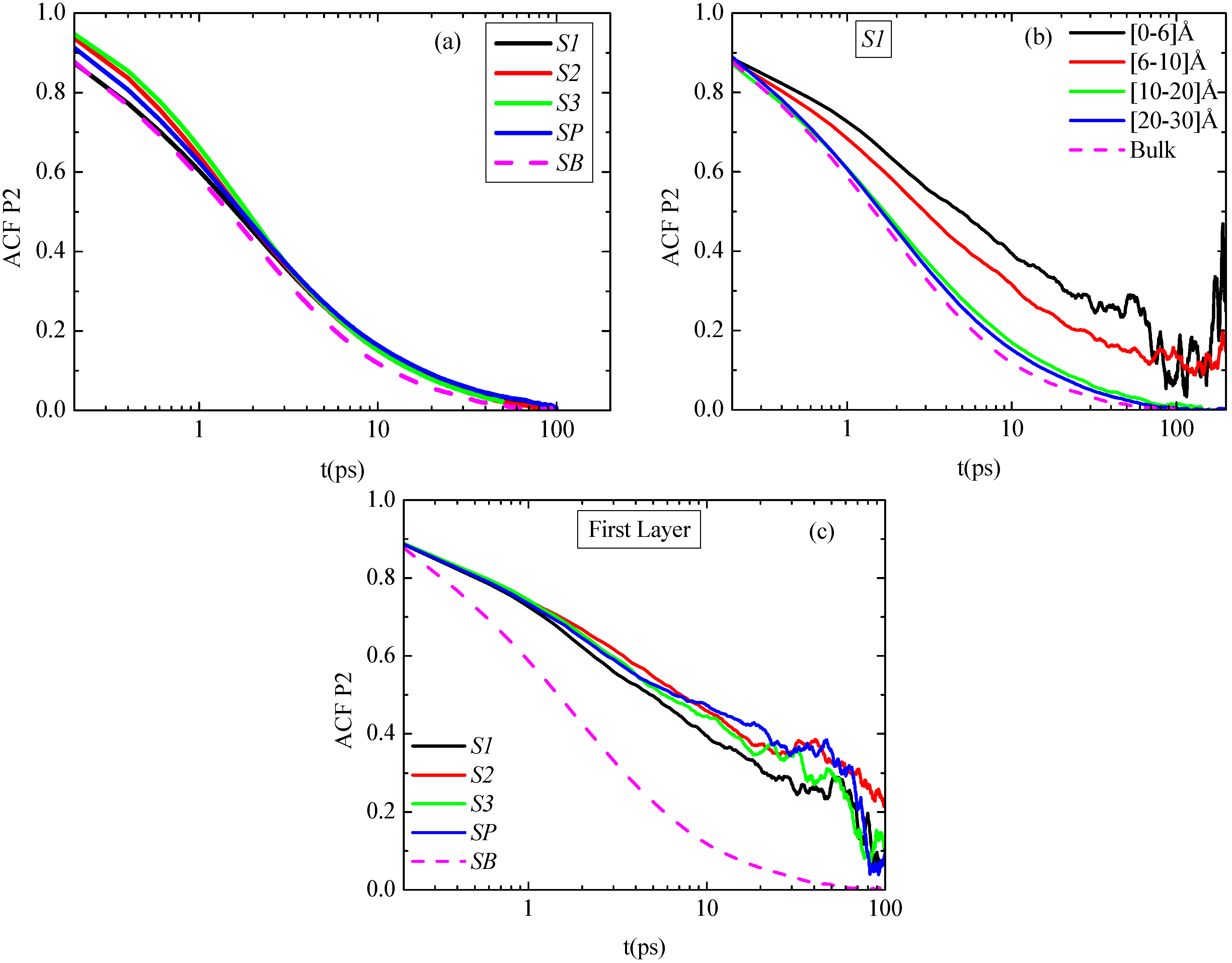
We continue the analysis of the model PNCs by presenting dynamical properties of PE as a function of the distance from the graphene layer. Using the time autocorrelation function (ACF) of the second Legendre polynomial:
, we first study the
orientational dynamics at the segmental level. The
v1−3 vector, which has been defined previously, is used and θ(
t) is the angle of this vector at time
t relative to its position at
t = 0. Results for the autocorrelation function,
P2(
t) are presented in
Figure 6a–c for all hybrid PE/graphene nanocomposites studied here. Corresponding data for a bulk PE system are shown in these Figures as well. Note that for these calculations we monitor the position of each segment/vector only for the time period it belongs to the corresponding analysis regime.
First, in
Figure 6a data concerning the
P2(
t) function of PE chains, averaged throughout the entire hybrid systems, are presented for the four nanocomposite systems as well as for the bulk PE system. There are only small differences between the different systems,
i.e., hybrid systems show a slightly slower average segmental dynamics compared to the bulk one. In more detail, at very short times
P2(
t) curve that corresponds to the system with the smallest graphene sheet (S1) coincides with the bulk one, while for the other three systems
P2(
t) curves attain higher values. This can be thought as a result of the fast motion of the very small sheet, which hinders the immediate effect on the polymer chains, so for a very short period they behave like being in bulk, but they diverge rapidly from this behavior.
Second, in
Figure 6b
P2(
t) at different radial adsorption layers (
i.e., different distances from the graphene sheet’s center) for the S1 system are shown. PE chains in the first adsorption layer show much slower segmental dynamics compared to the bulk one. A faster decorrelation is then observed moving away from the surface up to a specific distance, while beyond this all curves coincide. This distance determines the width of the PE/graphene interphase for the orientational segmental dynamics. Qualitatively similar data were found also for the other two hybrid PE/graphene systems (S2, S3). An extended interphase is also detected here as a result of the different kinetic behavior among the graphene flakes of various sizes. The width of the interphase is found to be rather similar to the one reported previously, concerning the distribution of the dihedrals angles.
Figure 6.
Time autocorrelation function (ACF) of bond order parameter P2(t) as a function of time for the characteristic vector v1−3 of polyethylene for all systems. (a) Average P2(t) values are over the entire system; (b) P2(t) values for the S1 system, for various spherical shells; (c) P2(t) values for all systems in the first adsorption layer. In all cases the corresponding bulk system is presented as well.
To further quantify differences, concerning the segmental dynamics of the PE chains in the vicinity of the PE/graphene interface,
P2(
t) for the first adsorption layer for all systems studied here are shown in
Figure 6c. It is clear that the relaxation of PE chains is much slower in all systems compared to the bulk case. In addition, there are small differences between the different systems; the S1 system exhibits slightly faster relaxation (larger mobility) compared to the S2 and S3 systems. Overall, in agreement to the structural characteristics of the hybrid systems, it seems that the behavior of the PE chains for the two larger systems is closer to the infinite one, whereas for the smallest system the differences are more pronounced.
Another important aspect concerns the examination of the polymer chain dynamics at the polymer/graphene interface of the PNC, compared to previous studies of PE/graphene thin films [
18,
20,
21]. Slight differences exist between the current study and our previous publications concerning PE/graphene systems (using a periodic and frozen graphene layer). In more detail data reported here show a slightly faster decorrelation of the
P2(
t) functionof
v1−3 vectors that are at the polymer/graphene interface (distances up to about 1 nm) compared to the frozen graphene sheets, whereas for longer distances relaxation times are identical for both cases. The analysis in the last studies was based on layers parallel to the graphene sheet and equidistant from the surface. For this reason we observed that at long distances the
P2(
t) curves overlap with the corresponding bulk curve. It is the periodicity of the sheet that favors this geometry in contrast to the present work where the finite size of the sheets demands a different geometric scheme for the analysis of the model configurations.
The effect of the PE/graphene interface on the PE segmental dynamics of each system can be further quantified by computing the corresponding segmental relaxation times, through proper fits of curves shown above (
Figure 6a–c), with a Kohlrausch–Williams–Watts (KWW) stretch exponential function [
29] of the form:
, where,
A is a pre-exponential factor which takes into account relaxation processes at very short times (e.g., bond vibrations and angle librations), τ
KWW is the KWW relaxation time and β the stretch exponent, which describes the broadness of the distribution of the relaxation times (
i.e., the deviation from the ideal Debye behavior—β = 1). Then, segmental relaxation time, τ
seg, is calculated as the integral of the KWW curves through:
where Γ() is the gamma function.
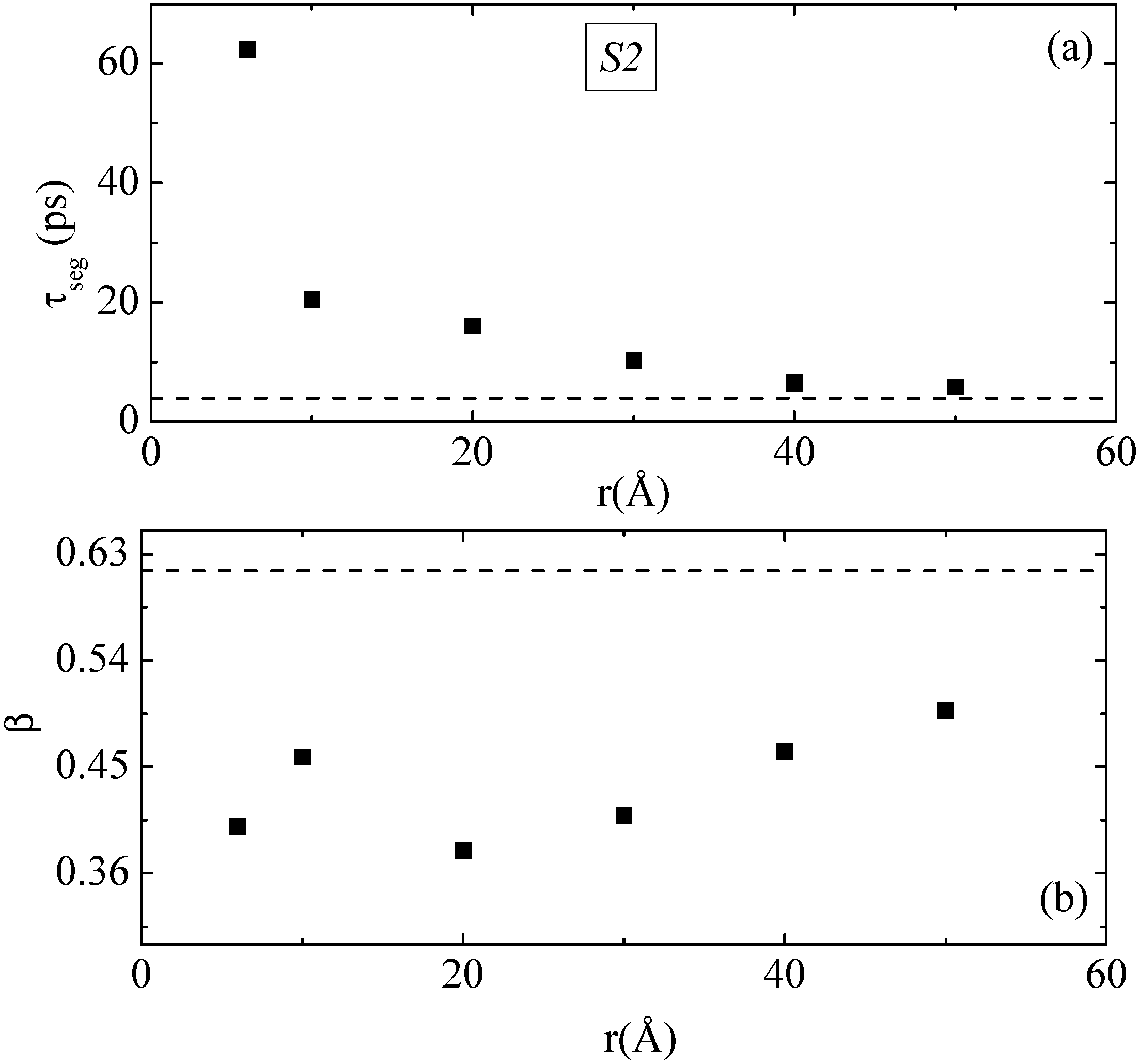
The results of the above analysis for both the segmental relaxation time τ
seg and the β exponent for PE chains of the S2 system are presented in
Figure 7a,b, respectively. Bulk values are also shown in this figure with dashed lines. It is clear the much slower orientational dynamics (larger segmental relaxation time τ
seg) of PE chains that are very close to the graphene layer (about 0.5 nm); τ
seg is about 10 times larger than the bulk one. As expected polymer segments become more mobile as their distance from the graphene layer increases, reaching a plateau, bulk-like regime, at distances of about 4.0–5.0 nm away from the graphene sheet. In addition, β-exponent values of PE chains at all distances are smaller than the bulk value (~0.62), shown in
Figure 7b with dashed line.
Qualitatively similar to the above behavior is also the case for the other systems studied here. In order to compare the behavior of the PE chains closest to the graphene layer we present in
Table 3 the τ
seg and the β exponent for the different systems in the first adsorption layer as well as for the bulk system. We observe that as the size of the graphene layer increases the relaxation time of the PE chains slightly increases,
i.e., their mobility becomes slower, for the cases of the finite graphene sheets. However, in periodic graphene a slightly smaller relaxation time, compared to the finite sheets, is observed, which can be attributed to the reduced motion of the periodic graphene’s center-of-mass. Values for the β exponent are similar for all systems (around 0.4), smaller than the bulk value of 0.62. The latter indicates a
broader distribution of the polymer segmental dynamics, compared to the bulk one, even for distances far away from the graphene sheets, where the
average τ
seg is similar to its bulk value. Therefore, when the way that polymer/graphene interfaces affect the dynamical properties of a PNC system is considered, average properties do not provide the full information, but rather the whole distribution of segmental dynamics should be examined. This results shows that dynamical heterogeneities present in polymer nanocomposites systems is an even more complex phenomenon than those appeared in polymer/solid interfacial systems (e.g., PE confined between graphene sheets [
18]), for which the behavior far away from the surface reaches the bulk one.
Figure 7.
(a) Segmental relaxation time, τseg, of v1−3 characteristic vector based on P2(t) time autocorrelation as a function of R (distance from the center of the graphene layer) for the S2 system; (b) The stretch exponent β, as extracted from the fit with KWW functions. Dashed lines represent τseg and β values of bulk PE under similar conditions (T = 450 K, P = 1 atm).
Table 3.
Average segmental relaxation times τseg and stretch exponents β of PE chains for all systems studied here (columns 2 and 3). τseg values and stretch exponents β for all systems in the first adsorption layer are shown in columns 4 and 5. Error bars are obtained using block averaging techniques.
| Systems | τseg-Average (ps) | β-Average | τseg-1st Layer (ps) | β-1st Layer |
|---|
| S1 | 4.6 ± 0.3 | 0.53 ± 0.05 | 44 ± 6 | 0.40 ± 0.05 |
| S2 | 6.7 ± 0.4 | 0.46 ± 0.05 | 62 ± 6 | 0.40 ± 0.05 |
| S3 | 6.1 ± 0.4 | 0.49 ± 0.05 | 63 ± 6 | 0.38 ± 0.05 |
| SP | 5.8 ± 0.4 | 0.52± 0.05 | 47 ± 5 | 0.41 ± 0.05 |
| SB | 3.9 ± 0.3 | 0.61 ± 0.05 | - | - |
In the next stage, we examine the
translational segmental dynamics of PE chains. To distinguish translational dynamics for different layers we have calculated the average segmental mean-square displacement (msd) defined as:
where
j is a specific radial region,
i is a particular segment (CH
2 or CH
3 group here) within region
j, r
i(
t) and r
i(
t + τ) are the coordinate vectors of segment
i at time
t and
t + τ, respectively, whereas brackets < > denotes statistical average. Note, that in the analysis used here a segment
i contributes to the above average msd for a given time interval
τ and for a radial region
j, if and only if it was constantly present in that region in the entire course of time
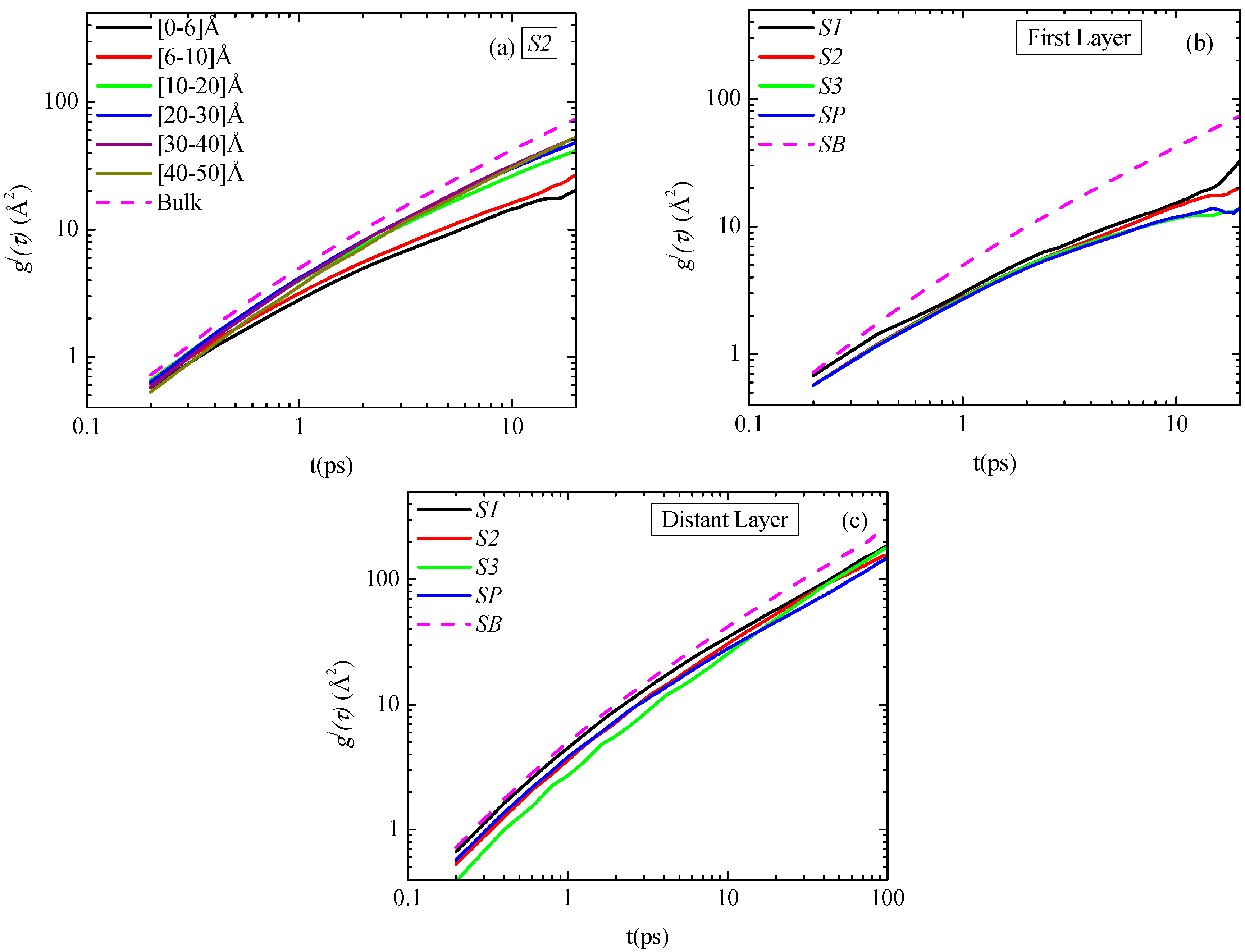
τ. First, in
Figure 8a data concerning
gj(τ) for all (radial) adsorption layers for the S2 system are shown. The segmental dynamics of the polymer atoms that are closer to the graphene sheet atoms (mainly in the first two adsorption layers) is slower compared to the one of the atoms in the other layers. On the contrast, segments belonging to the other regimes, (above second layer) exhibit rather similar dynamics, which is slightly slower to the bulk one, shown in
Figure 8a with dash line.
In
Figure 8b data concerning
gj(τ) for the first adsorption layer (
j = 1) for all systems studied here are presented. It is clear that the segmental dynamics of the PE chains closest to the graphene layers is slower, compared to the bulk one, for all model PNCs systems. In addition, there is a slight dependence of the PE segments
gj(τ) msd on the size of the graphene sheet mainly in the
~5–20 ps time regime,
i.e., the segmental dynamics for the small-graphene system (S1) is faster than the two other systems, whereas
gj(τ) for the biggest graphene system (S3) is similar to the periodic-infinite case. In
Figure 8c
gj(τ) msd data for PE chains belonging in a radial layer far away from the graphene sheet are shown for all systems. Segmental translational mobilities of different systems are very similar to each other, slightly slower than the unconstrained bulk one.
Figure 8.
(a) Segmental mean squared displacement for polyethylene chains along R (distance from the center of the graphene layer); (a) Values for the S2 system, for various spherical shells; (b) Data for the first adsorption layer (distant layer) (R = 0.6 nm) for all systems; (c) Data for the last adsorption layer (R = LBOX/2) for all systems. In all cases the corresponding bulk curves are included.
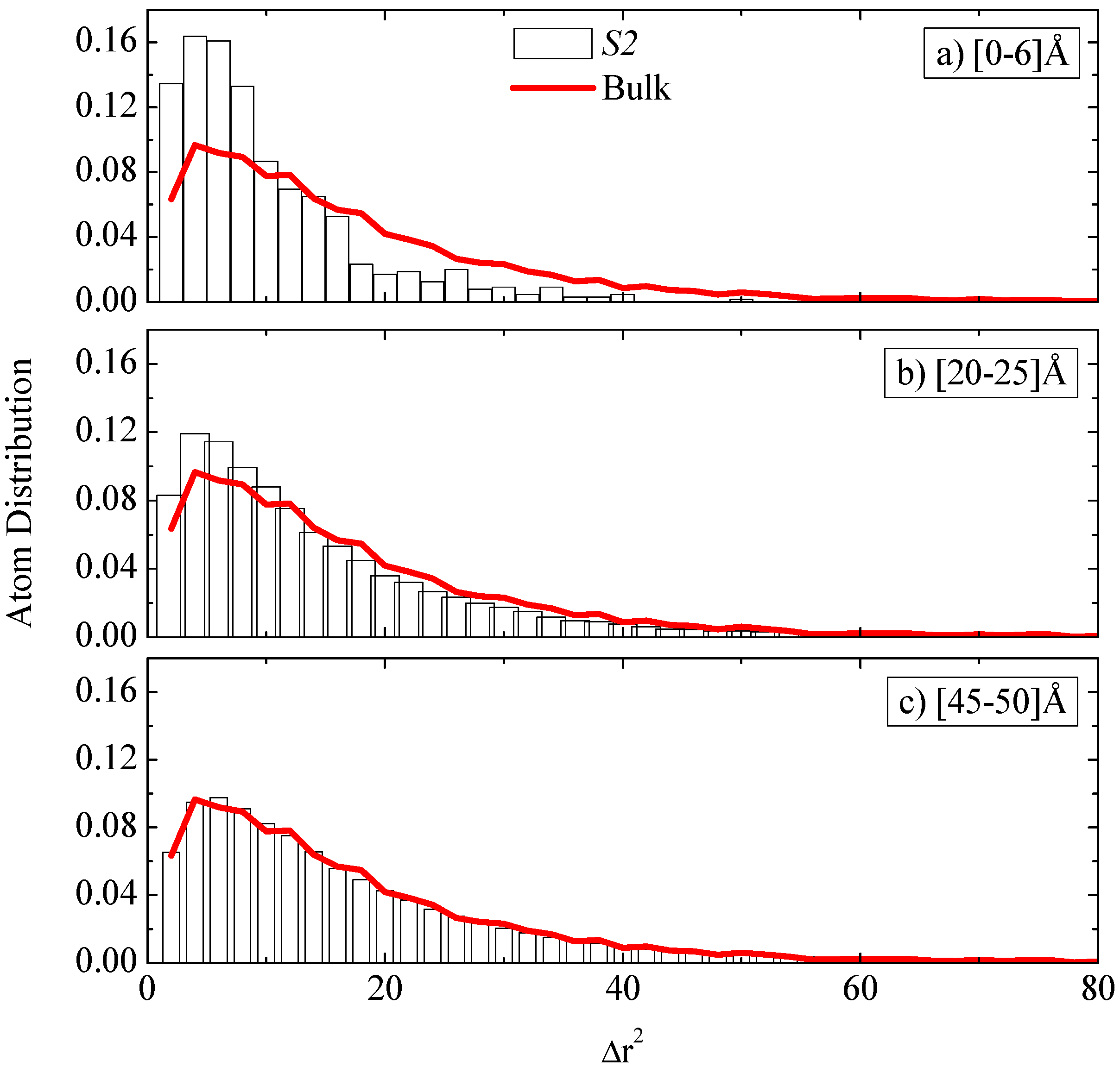
The
dynamical heterogeneity of polymer atoms discussed above can be examined in greater detail if we consider the probability distribution of segmental
gj(τ) msds for a specific time period τ. An important aspect is related to the disturbance of such a distribution, compared to the bulk polymer system. Data for the distribution of
gj(τ) for the S2 system and a specific time period similar to the bulk segmental relaxation time (τ
= 5 ps) are shown as bars in
Figure 9a–c for three different radial regimes: 0–6 Å, 20–25 Å and 45–50 Å. In all cases the distribution of a bulk system is shown with a solid line. First, a broad distribution is shown for all regimes, especially for the second and third regime shown here (
Figure 9b,c), for which msds have been found in the range 0–80 Å
2 similar to the one of the bulk system. Segments in the first regime (atoms closest to the graphene sheet) show a more narrow distribution, with msds in a 0–40 Å
2 range. Second, the probability distribution of
gj(τ) msd’s, of atoms belonging in the first adsorption regime (
Figure 9a), is larger than the bulk one for small displacements (Δ
r2), up to about 10 Å
2. On the contrary, the probability to find larger msds, above about 10 Å
2 is smaller than the bulk one. As we move far away from the graphene sheet the probability distribution of the
gj(τ) msd’s data approaches the bulk one,
i.e., probability of finding small msds decreases, whereas the probability to find larger msds increases. This is particular clear for the longer distances 45–50 Å, which exhibit very similar distribution to the bulk PE atoms.
Figure 9.
Probability distribution of the mean squared displacements, gj(τ), for the S2 system at a specific time period (τ = 5 ps) for three different radial regimes: (a) 0–6 Å; (b) 20–25 Å and (c) 45–50 Å. In all cases the distribution of a bulk system is shown with a solid line.
Figure 9.
Probability distribution of the mean squared displacements, gj(τ), for the S2 system at a specific time period (τ = 5 ps) for three different radial regimes: (a) 0–6 Å; (b) 20–25 Å and (c) 45–50 Å. In all cases the distribution of a bulk system is shown with a solid line.
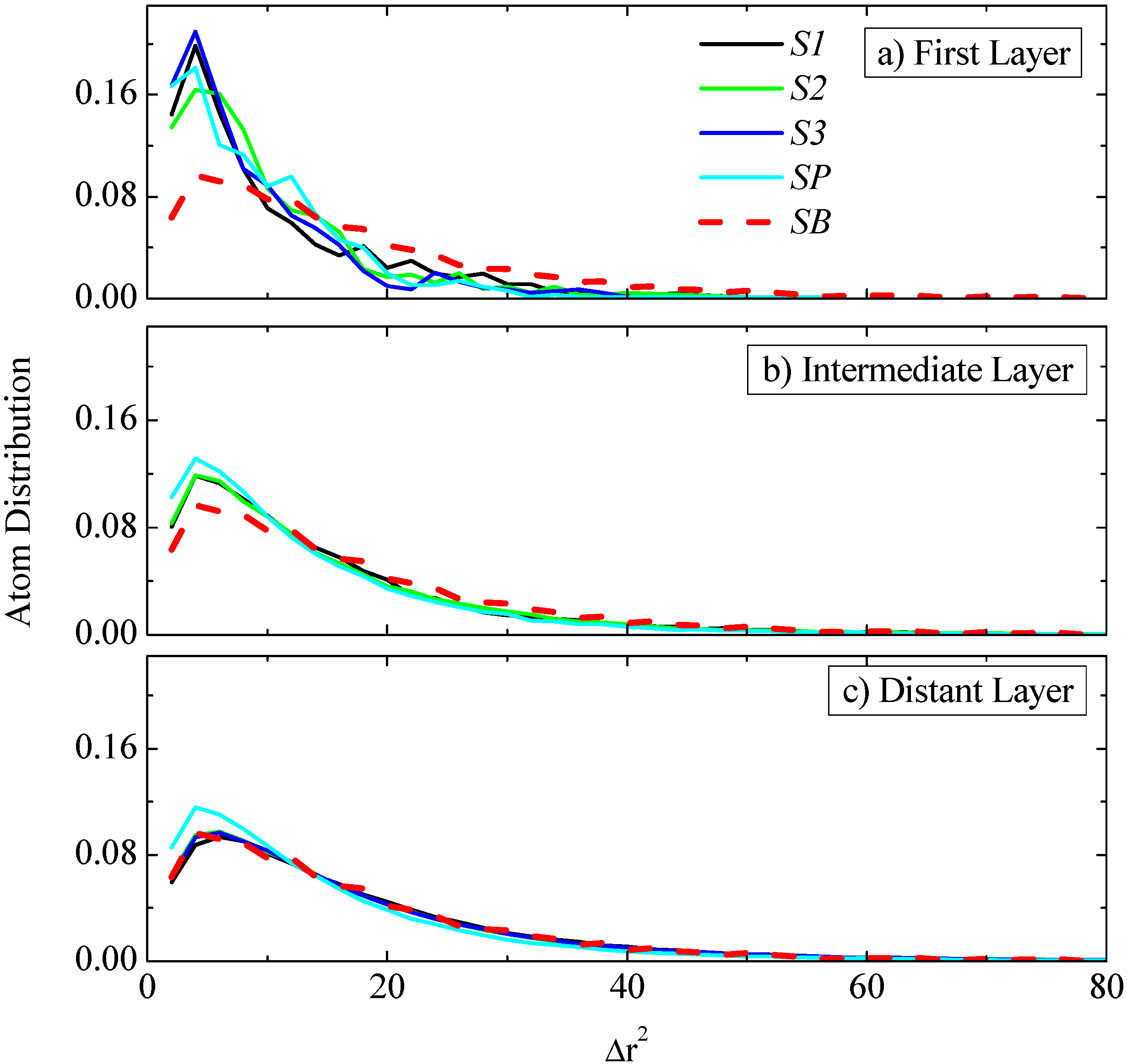
Data concerning the probability distribution of
gj(τ), computed at three different regimes and for the specific time period discussed above (τ = 5 ps), are shown in
Figure 10a–c for all S1, S2 and S3 systems, respectively. All systems exhibit a similar behavior to the S2 system discussed above (see
Figure 9);
i.e., for segments belonging to the radial regime closest to the graphene surface there is a larger probability for smaller msds, compared to the bulk one. This is in agreement with the average
gj(τ) data presented above in
Figure 8a–c. On the contrary, segments belonging to the regime that is far away from the graphene sheet show similar distribution to the bulk system. In the same graph the distribution for the infinite-periodic system (SP) is shown as well. The latter exhibit qualitatively similar behavior as expected. There is only a small difference in the far distant layer for the SP system that still exhibits larger (smaller) probabilities for small (large) distances, compared to the bulk one. The reason for this difference is that due to the “infinite” size of the periodic graphene layer there are always some atoms in the radial analysis used here that are in small distances from the graphene atoms. The msds of these atoms is on the average smaller; thus increasing the probability to find smaller msds in the graphs shown in
Figure 10c.
Figure 10.
Probability distribution of the mean squared displacements, gj(τ), for all three systems at a specific time period (τ = 5 ps) for three different regimes: (a) First layer: 0–6 Å; (b) intermediate layer: (10–15 Å for S1, 20–25 Å for S2, 30–35 Å for S3, 15–20 Å for SP) and (c) distant layer: (25–30 Å for S1, 45–50 Å for S2, 65–70 Å for S3, 35–40 Å for SP). In all cases the distribution of a bulk system is shown.


