Abstract
The impact of phase morphology in electrically conducting polymer composites has become essential for the efficiency of the various functional applications, in which the continuity of the electroactive paths in multicomponent systems is essential. For instance in bulk heterojunction organic solar cells, where the light-induced electron transfer through photon absorption creating excitons (electron-hole pairs), the control of diffusion of the spatially localized excitons and their dissociation at the interface and the effective collection of holes and electrons, all depend on the surface area, domain sizes, and connectivity in these organic semiconductor blends. We have used a model semiconductor polymer blend with defined miscibility to investigate the phase separation kinetics and the formation of connected pathways. Temperature jump experiments were applied from a miscible region of semiconducting poly(alkylthiophene) (PAT) blends with ethylenevinylacetate-elastomers (EVA) and the kinetics at the early stages of phase separation were evaluated in order to establish bicontinuous phase morphology via spinodal decomposition. The diffusion in the blend was followed by two methods: first during a miscible phase separating into two phases: from the measurement of the spinodal decomposition. Secondly the diffusion was measured by monitoring the interdiffusion of PAT film into the EVA film at elected temperatures and eventually compared the temperature dependent diffusion characteristics. With this first quantitative evaluation of the spinodal decomposition as well as the interdiffusion in conducting polymer blends, we show that a systematic control of the phase separation kinetics in a polymer blend with one of the components being electrically conducting polymer can be used to optimize the morphology.
1. Introduction
Electrically conducting polymers have created many success stories in the commercial world of electronics. Organic light-emitting diodes, photon-harvesting components in organic photovoltaics, hole-transport layers, and also components in organic field-effect in transistors are all results from the great invention of doping semiconducting polymers by Heeger, MacDiarmid, and Shirakawa in the late 70’s [1]. The enhanced solubility and processability of these electroactive polymers have yielded the understanding of the impact of the resulting morphology in their composites and blends. The phase separation and interdiffusion of the poly(3-hexyl)thiophene (P3HT) have also become essential control parameters in bulk heterojunction organic photovoltaics [2]. Chen et al. [2] discussed how the mixture of P3HT with modified C60 was shown to be highly miscible and eventually separated in nanoscopic, bicontinuous morphology after annealing at elevated temperatures. The further crystallization of P3HT was shown to have an additional importance at the end of exciton migration in the performance of the solar cells.
We applied an “electroplating” approach to build organic solar cells on various shapes of surfaces by polymerizing electrochemically the organic components on the transparent electrodes [3,4,5,6]. In spite of the excellent developed nano-structured hole-transport layer, the efficiency of the organic solar cell was not improved with the annealing step because of the limited crystallization of the electropolymerized polymers with the high degree of crosslinking. In order to obtain improved understanding for obtaining the needed bicontinuous morphology in the bulk heterojunction solar cells, we decided to conduct a model study for the behavior to thiophene polymers in a two-polymer, thermoplastic blend. According to our previous studies, poly(3-dodecylthiophene) (P3DDT) was shown to be miscible with poly(ethylene-co-vinylacetate), with vinylacetate content 20% (EVA 20), up to a composition of 30% P3DDT [7,8]. The driving force for the miscibility is the interaction between the components resulting in conformational changes in the P3DDT backbone. The decrease in the length of the conjugated segment is related to the planarity of the polymer backbone structure. This observed change was evidenced as a solvatochromic shift in the UV-spectrum, when diluting P3DDT in the EVA 20 matrix in the miscible region [7,8]. This confirmed initial state of miscibility in the polythiophene blends gave us the motivation for the fundamental approach investigating the phase separation and interdiffusion processes as shown in Figure 1.
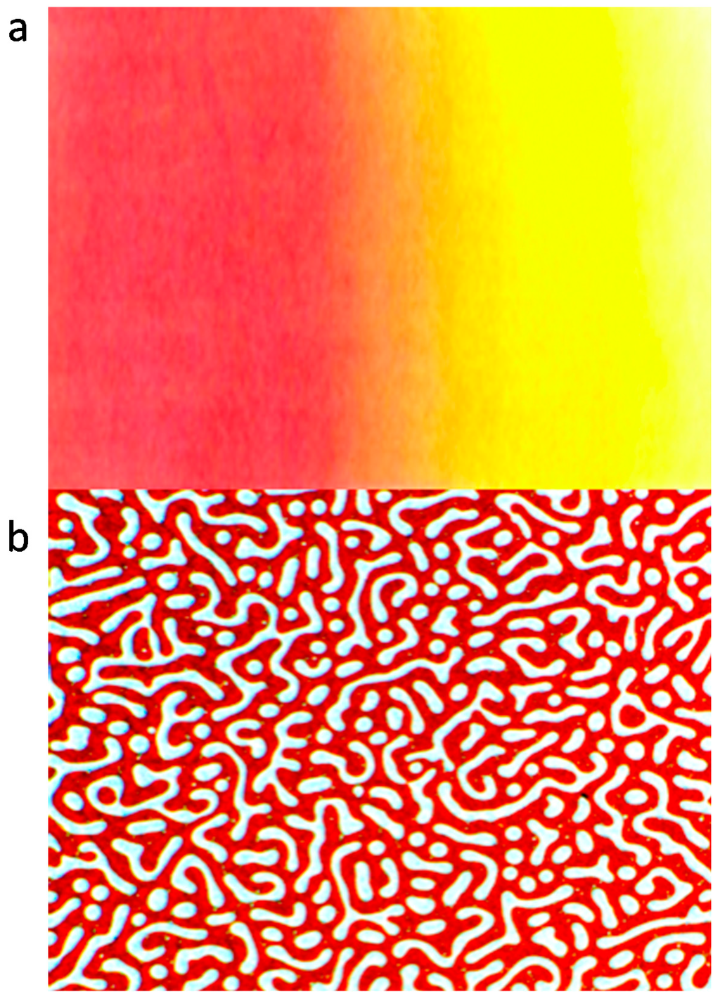
Figure 1.
Optical microscope pictures of inter-diffusion (a) and phase separation (b) of polyalkylthiophene blends.
Figure 1.
Optical microscope pictures of inter-diffusion (a) and phase separation (b) of polyalkylthiophene blends.

Figure 1a presents the concentration profile/gradient after a certain time of interdiffusion of the two components to a single, miscible phase and Figure 1b a bicontinuous morphology after a controlled phase separation from a miscible P3DDT blend. The pictures presented are purely schematic for guidance and both phenomena are discussed with experimental details in this manuscript. P3DDT has an absorption maximum at around 490 nm measured by UV spectroscopy revealing red color in a solution or on a thin film, with dilution, the color changes to yellow due to the solvatochromic effect. The miscibility of two (or more) polymers depends on the thermodynamic stability of the phase state and can be studied from the thermodynamic point of view by understanding the thermodynamics of mixing. If two polymers have a partial miscibility with lower critical solution temperature (LCST) behavior, the homogeneous blend can decompose to two separate phases by the nucleation and growth (NG) or by the spinodal decomposition (SD) mechanism depending of the temperature and the composition of the blend. In the early and in the intermediate stages of the SD, the structure of the phases is bicontinuous; one insulating polymer rich phase and the other conducting polymer rich phase. This kind of behavior is one proposed explanation for a multiple percolation concept, which can be used to reduce the amount of the conducting polymer in polymer blends [9]. The classical percolation theory persists that the conductivity is achieved when the critical volume fraction of the conducting polymer, φc, is ~16%. By using multiple percolation concept the conductivity can be achieved with φc ~3% in a binary blend. In Figure 1b the paths are already disconnected by the coarsening and ripening process in the later stage of SD. This breaking of the continuous clusters to the discrete droplets was envisaged by Reich as a percolation process by reversing the time arrow [10].
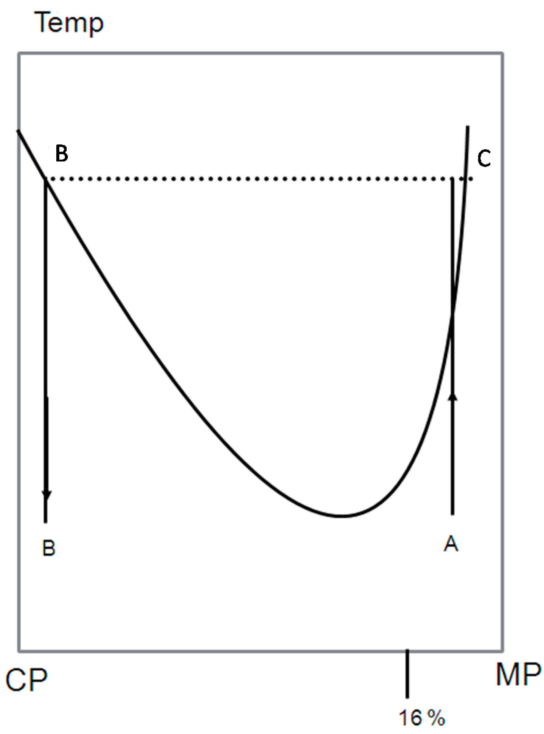
A schematic LCST phase diagram is shown In Figure 2 to illustrate double percolation. The blend is made of the conducting polymer (CP) and the matrix polymer (MP), which is insulating polymer. Because the starting composition φ0 in the mother phase A in Figure 2 contains less than 0.16 volume fraction of CP, the mother phase is not conducting. After phase separation, the mother phase has decomposed into two phases B and C. The phase B has a composition φb, which volume fraction of CP is more than 0.16, and thus, it must be conducting. There is also additional requirement for conduction of the whole blend: the phase B itself must also be connected. This kind of percolation inside percolation is called double percolation.
The connected paths of the phase B can be created by spinodal or nucleation and growth. After the required conditions of the connected paths are achieved, the phase must be “locked” in such a composition. This can be done by cooling the blend to glassy state (below the glass transition temperature) accompanied by crystallization, before the coarse-graining occurs. The resulting of the blend preserves the desired connectivity and conductivity properties. By this method conductivity can be reached by 0.03 volume fraction of CP, which is much less than the classical theory predicts [9].

Figure 2.
Schematic phase diagram with a lower critical solution temperature presented to illustrate double percolation. A, initial miscible composition; B, phase separated composition with high CP concentration; C, phase separated composition with low CP concentration.
Figure 2.
Schematic phase diagram with a lower critical solution temperature presented to illustrate double percolation. A, initial miscible composition; B, phase separated composition with high CP concentration; C, phase separated composition with low CP concentration.
If we denote the critical volume fraction of CP in the B required for conductivity φCP and the critical volume fraction of phase B in the blend required for B itself to be connected as φB, then the critical volume fraction of CP in the blend φC can be expressed as:
φC = φB·φCP
To reach the connected paths, both φB and φCP must be ~0.16 in binary blend [9]. Thus, the φC is ~0.028.
The Equation (1) can be easily generalized for multiple percolation. If there is n levels of connected paths each inside the other, only the last of which is required to actually be conductive, φC can be expressed as:
φC = φCP·φBn−1
In ternary blend Equation (2) gives us result φC = 0.004. This estimate defines an upper boundary for the CP content since this approach is based on spherical particles. In reality, anisotropic shapes may appear in the morphology and the effect of those changes will make the required CP content even smaller as is well-known from percolation theory. If anisotropic shapes appear in any level of the multiple percolation hierarchy, the appropriate numerical estimate of the percolation threshold needs to be substituted instead of spherical φB and φCP in Equations (1) and (2). The estimate of the multiple percolation threshold introduced in the Equation (2) represents only a rough estimate and reflects the notion of the statistical independence of the levels in multiple percolation [9].
Poly(3-alkylthiophene)s have partial miscibility with EVA, if the vinylacetate content of the EVA is less than 40% and the composition of thiophene in the blend is smaller than 30% [7,8]. A phase diagram is shown in the Figure 3 based a cloud point (A–C for compositions 15/85, 20/80 and 25/75) and the melting temperature measurements (E) for poly(3-octylthiophene) (P3OT) and EVA20 blends [7,8]. The cloud point B for 20/80 composition (P3OT/EVA20) was obtained at 132 °C and A for 15/85 composition at 180 °C. The 10/90 composition does not reveal any evidence for phase separation when heated to 200 °C. Above this temperature the thermal degradation starts to interfere. The 30/70, 40/60, and 50/50 composition blends formed uniformly colored films, which phase-separated when heated above the melting point of the EVA20. Point D in the phase diagram for composition 40/60 presents a phase-separated structure already at room temperature (RT) [7,8]. The semitransparent arrow presents the direction of the temperature jump experiments described later.
The phase separation can take place two different ways depending on composition, temperature, and pressure; by nucleation and growth or by spinodal decomposition in which structures coarsen by an interfacial energy-driven viscous flow mechanism [11,12]. The intermediate demixed structures are expected to be quite different for these two mechanisms. In the early NG stage, the nuclei with equilibrium composition in the mother phase with average composition is formed by the thermal activation process. The nuclei larger than the critical nucleus size will spontaneously grow. As the nucleation process proceeds, the composition of the nucleus stays constant; instead the composition of the mother phase approaches the equilibrium composition. The composition difference is controlled by the thermodynamic conditions of the mixture. The average size of the nuclei is determined by the kinetics, i.e., by the time of the process.
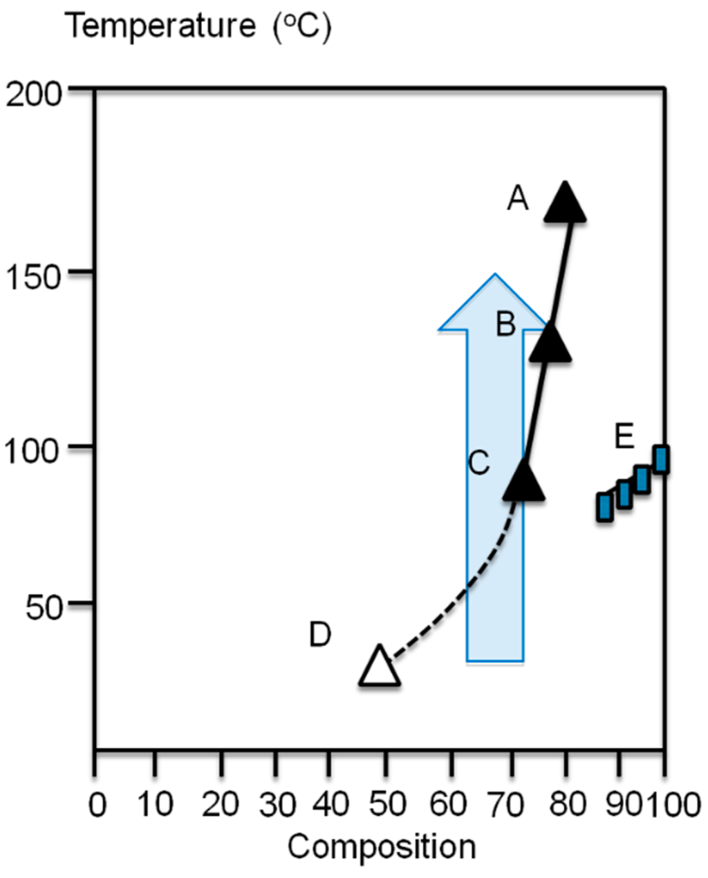
Figure 3.
The phase diagram of the P3OT/EVA20 blend.
Figure 3.
The phase diagram of the P3OT/EVA20 blend.

In the early SD stage the oscillating composition field is set up and the concentration fluctuations start to grow with time, i.e., the amplitude grows, while the wavelength is nearly constant. The wavelength is controlled by the thermodynamics conditions of the mixture, characterized by the “quench depth”, i.e., either by supercooling or by supersaturation. The amplitude of the fluctuations are controlled by the kinetics, i.e., by the time for the phase separation. Thus, the control of the size of the nuclei and the amplitude of the fluctuations are just opposite of those in NG regime. Since the mid-seventies, many authors have studied SD by wide and small angle light scattering (WALS and SALS, respectively) [13,14,15,16,17,18,19,20,21,22,23,24,25,26,27,28,29,30,31], by optical microscope (OM) [22,23,24,25,26,27,28,29,30,31], by pulsed nuclear magnetic resonance (NMR) [29], by small angle neutron scattering (SANS) [31], and by small angle X-ray scattering (SAXS) [32]. In this paper the main attention is paid for WALS, SALS, and OM.
The poly(3-dodecyl thiophene) (P3DDT)/EVA20 blend was prepared via solvent casting for the 20/80 and 25/75 compositions. The cloud point temperatures were measured as the function of three different heating rates and the confirmed temperatures for PDDT/EVA20 blend at compositions 20/80 and 25/75. The corresponding Tcp’s are 109.0 and 103.9 °C respectively. Temperature jump (Figure 3, semitransparent arrow) was initiated to a temperature where the phase separation was expected to occur based on the cloud point measurements. First, the phase separation was monitored using optical microscope. Optical microscope pictures show qualitatively the development of the morphology of the PDDT/EVA20 film with the composition of 25/75 at 130 °C. For quantitative measurements we used SALS technique to monitor the kinetics with so-called spinodal ring when the connected intermediate structure changes to separate droplets, the spinodal ring vanishes. Time-evolution SALS patterns of the spinodal region under reveals an isotropic “spinodal ring” scattering pattern is observed in the early stage of the phase separation when the domain formation is independent of the azimuthal angle and can be attributed to the concentration fluctuation. Within this period, the corresponding OM images show a bicontinuous phase structures. According to the Cahn-Hilliard linearized theory, the change of the elastic scattered light intensity IVv with time arising from the concentration fluctuation is related by:
where R(q) is the growth rate of the Fourier component of the fluctuations with q, the wave number of the sinusoidal composition fluctuations. The plot lg (IVv) vs. time will yield 2R(q), which is given by the slope. If this is done at various angles at the constant temperature, repeated with various temperatures and the results are plotted in the form of (R(q)/q2) vs. q2, this will yield (R(q)/q2) = Dapp by extrapolating q2 to zero.
IVv ~ exp[2R(q)t]
The spinodal temperature Ts can be estimated from the plot Dapp vs. temperature by extrapolating Dapp to zero. By doing this over the whole composition range, the spinodal curve can be estimated [25]. The kinetics of the phase separation for blend 20/80 were measured at 119, 120, 121, 122, 127, 128, and 130 °C and for 25/75 blend at 120, 121, 122, 123, and 130 °C. Figure 4 shows the linear behavior for (R(q)/q2) vs. q2 as expected for the spinodal region. The diffusion coefficient obtained from Figure 5 can then be used to estimate the spinodal temperatures. As seen in Figure 5, the spinodal temperatures for the two compositions are around 118–120 °C.
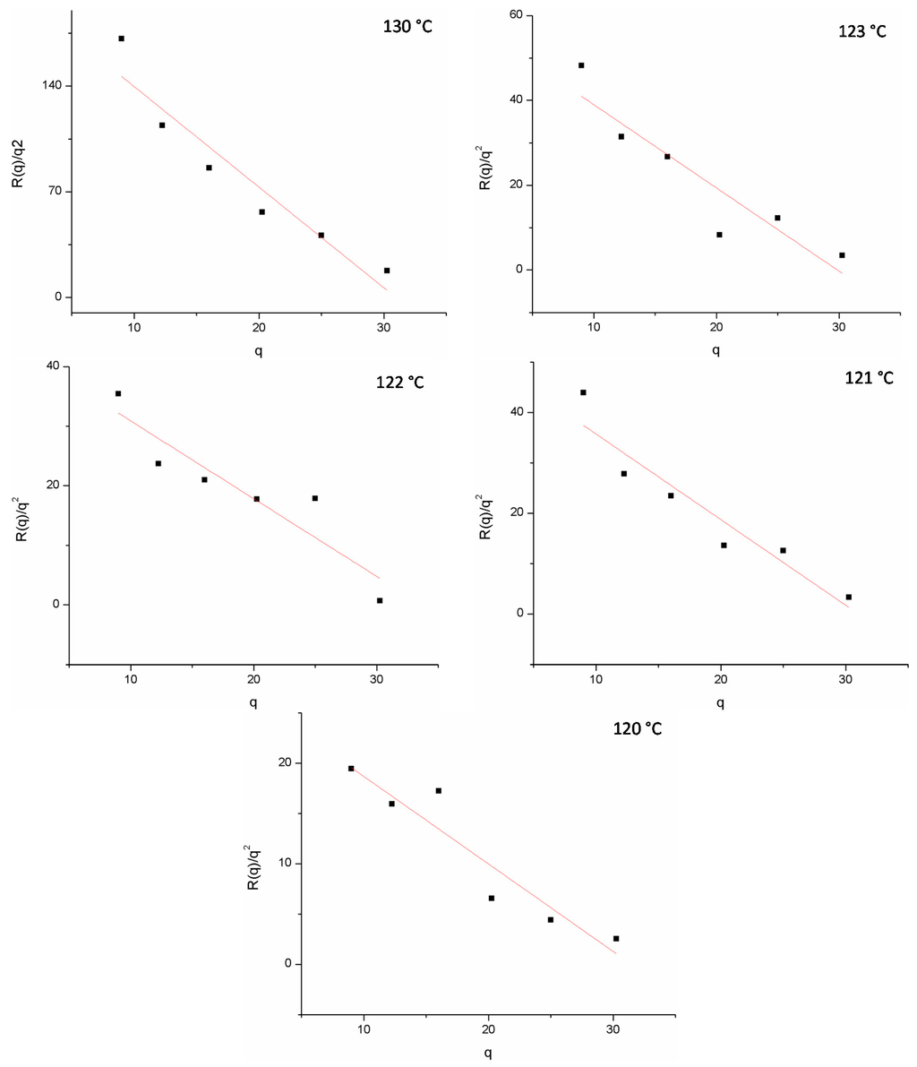
Figure 4.
Linear relation between R(q)/q2 and q.
Figure 4.
Linear relation between R(q)/q2 and q.
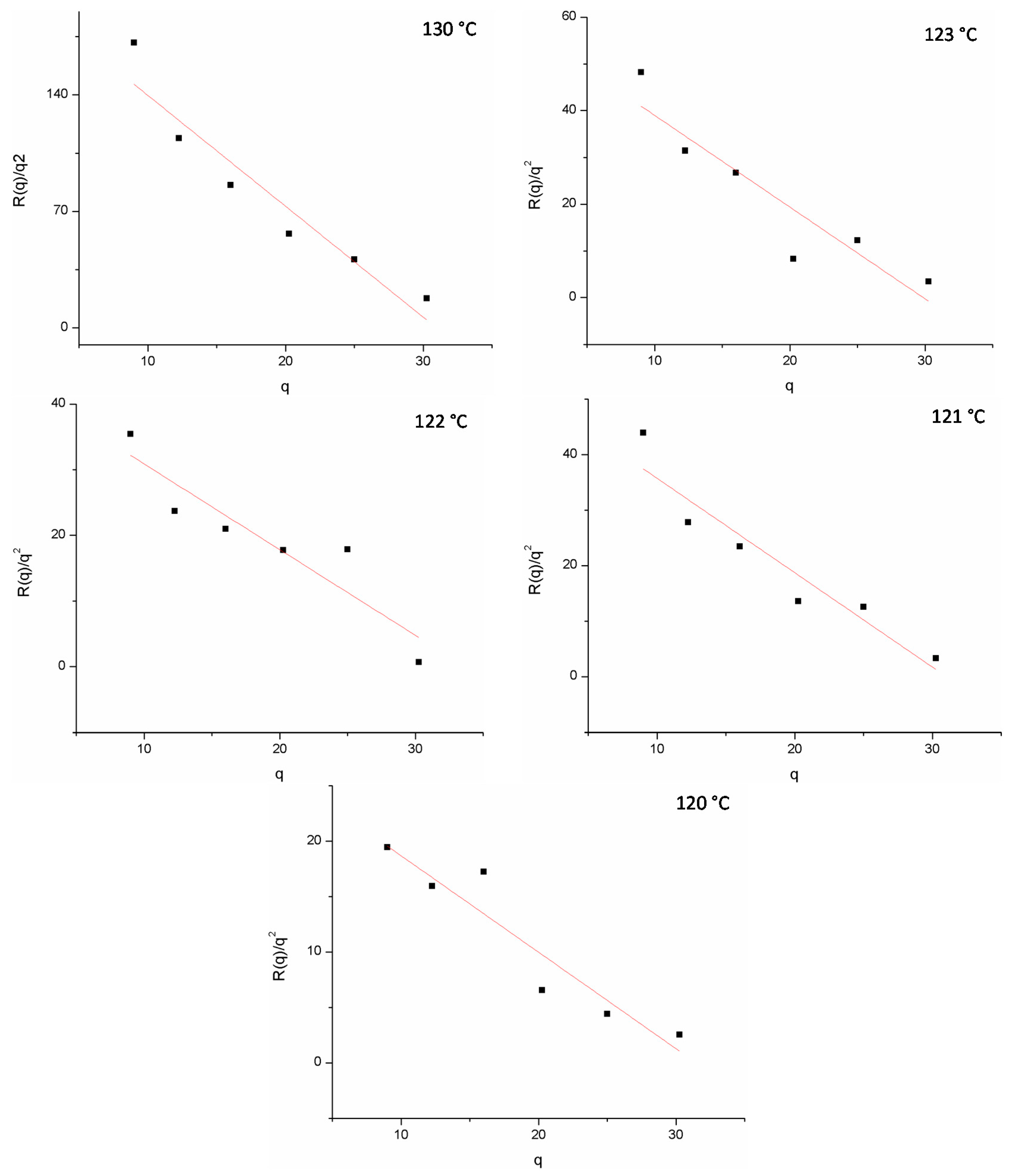
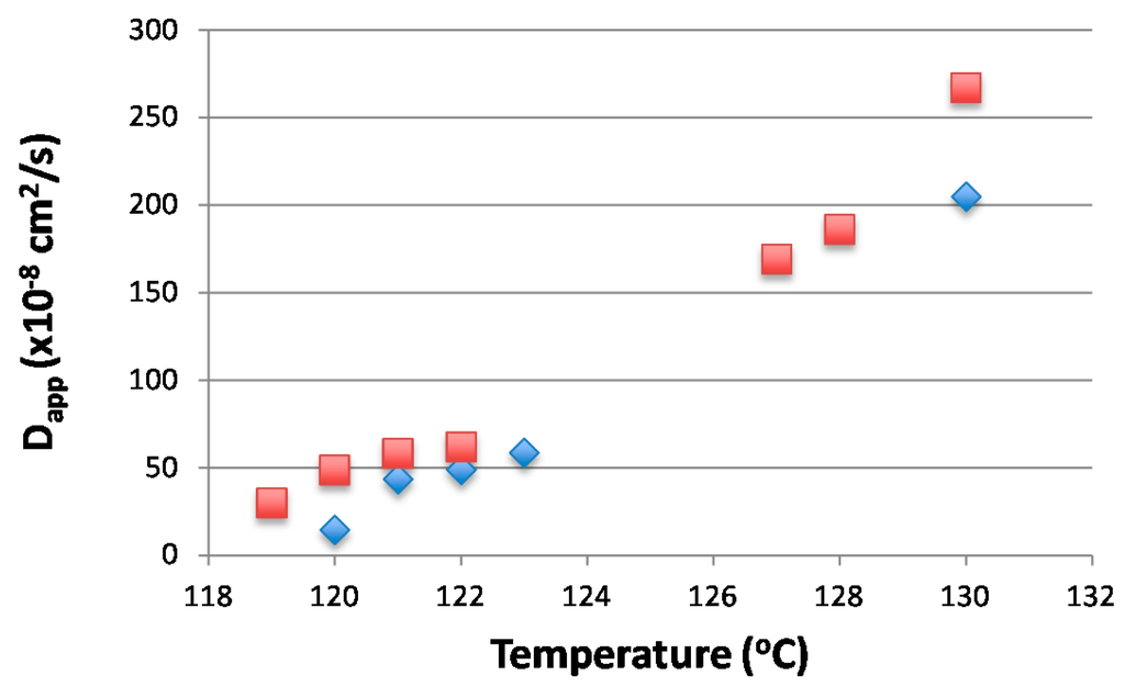
Figure 5.
The diffusion coefficients at measured temperatures (20/80 Blend Square, 25/75 Blend in Diamonds).
Figure 5.
The diffusion coefficients at measured temperatures (20/80 Blend Square, 25/75 Blend in Diamonds).

2. Spinodal Decomposition and Conductivity
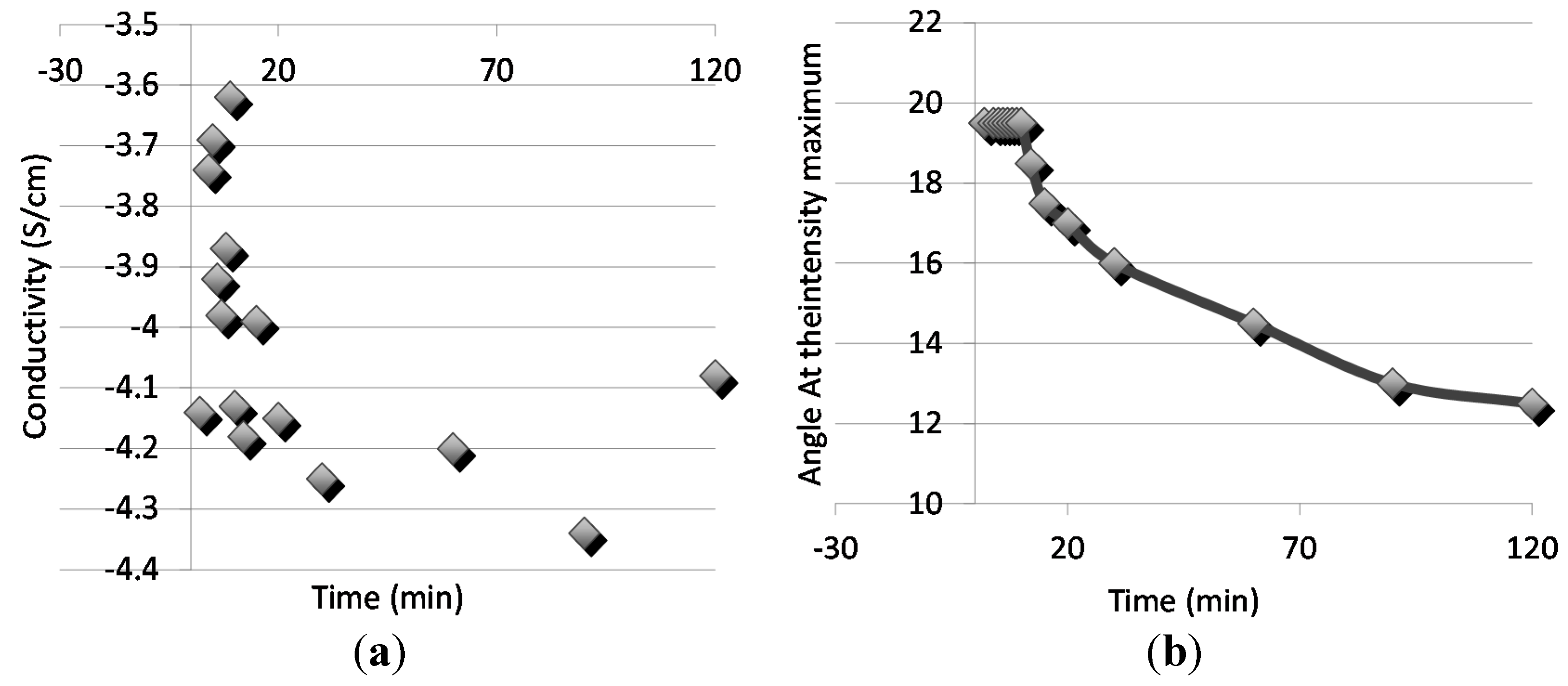
A classical percolation theory persists, that the conductivity is achieved when the volume fraction of conducting polymer fc in binary system is 0.16, if the conducting polymer exists as hard-core spheres. The polythiophene polymers in the blends were then doped with FeCl3 as explained the experimental section and the conductivities of the films were e then measured with the four-probe method. The doping was done to all the phase separated samples, thus the conductivities were measured with the kinetics of phase separation. The sequence is due to the fact that doped polymers would not have the diffusional properties needed for the kinetic observation due to the highly charged nature of the doped samples. Figure 6 relates the scattering angle (Figure 6a) and the conductivities (Figure 6b) with the phase separation time. Although the mixing was done in the undoped state, the relation of conductivity with the phase separation reveals interesting data. Initially before the phase separation, conductivities are at the same level as with the insulating polymer alone. In the early phase separation, in the spinodal region, where the scattering angle remains constant, a distinguished increase in conductivity is observed as a result of percolation of the conducting polymer rich phase. This may additionally be due to the continuing composition change packing the chains in ordered manner and impacting the charge transfer.

Figure 6.
(a) Conductivity and (b) the scattering angle with the time for the phase separation.
Figure 6.
(a) Conductivity and (b) the scattering angle with the time for the phase separation.
3. Interdiffusion of P3DDT and EVA Polymers
Interdiffusion has an effect on many physical properties, but the most direct information of the interdiffusion can be obtained by using experiments that yield concentration profiles across an interface. The detailed shape and the width of such profiles and the way these vary with time comprise in principle all the information on the interdiffusion process. They show how the interdiffusion rate varies with local composition, from which the molecular mechanisms that control it can be derived. Transmission Fourier transform infrared spectroscopy (FTIR) has been used to study mutual diffusion between poly(ethylene-co-methacrylic acid) and Poly(vinyl methylether) (PVME). The observation of the interdiffusion is due to the specific interaction between these polymers; the carboxylic acid and the ether groups interact forming a “free” carbonyl group. Attenuated total reflection infrared spectroscopy (ATR-FTIR) has been used to study interdiffusion between polymer couples polystyrene (PS) with PVME [33]. ATR-FTIR has several advantages: the interdiffusion can be measured in situ (reducing the sampling error), and the diffusion can be monitored without labeling (both polymers must have specific absorption bands in the IR region). We have applied UV spectroscopy similarly to follow the interdiffusion without using any additional labeling system.
The films of two polymers which were mechanically placed on top of each other on the glass micro slide were then heated and the inter diffusion started to occur when the temperatures were above the glass transition and melting (EVA20 89 °C and PDDT 139 °C) temperatures of the polymers and the sharp interface progressively disappeared. The observation revealed that colorful PDDT was diffusion into the EVA20 matrix.
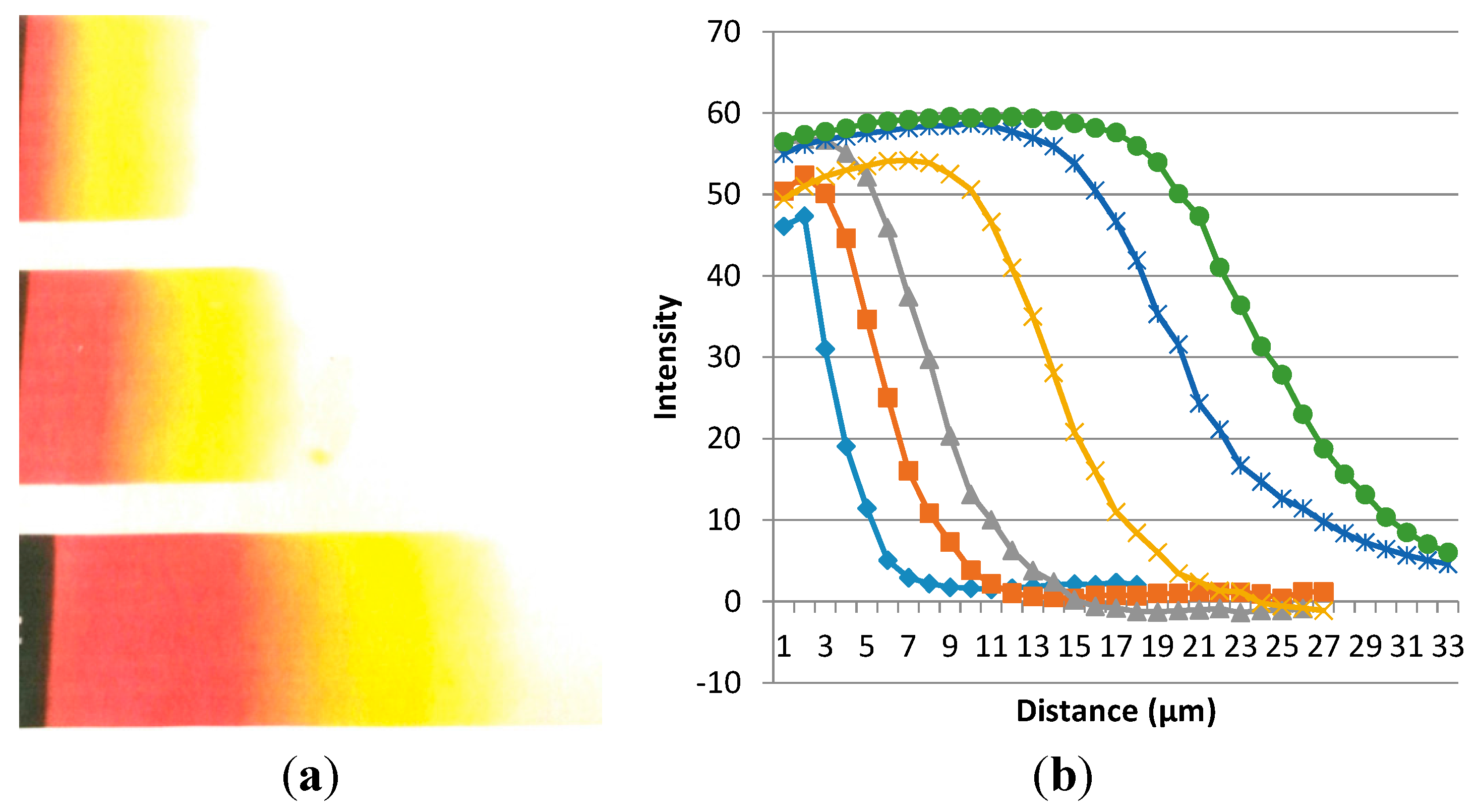
EVA20 and PDDT have a narrow miscibility window [7], mainly due to the “similarity” of the chemical structure: both polymers have about 80% hydrophobic components when the backbone and side chains chemical components are included. In addition the polar components may have weak polar interactions between them enhancing the miscibility. Figure 7A shows a typical result on the diffusion evaluation at room temperature for the heating experiment after the temperature reached 160 °C. It is obvious that the diffusion distance is dependent on the heating time suggests that the longer heating the longer the heating distance becomes. The color in the beginning of the diffusion is red/orange or and with the diffusion distance growing the color becomes lighter and lighter yellow. The color is an indication of PDDT concentration and the chromaticism (color change) reveals conformational changes with the dilution. Similar process has been evidenced with conducting polymer solutions and is called solvatochromism.
The concentration profiles shown in Figure 7a were then processed using Image-Pro Plus software. The digitized profiles of intensity/distance relation are shown after taking the pictures at 140 °C and between 30 and 240 min time intervals. The first horizontal line shows that all light passes through before any inter-diffusion occurs. With the evolution of the red/yellow color, less light is transmitted and the profiles show the diffusion with time and distance.
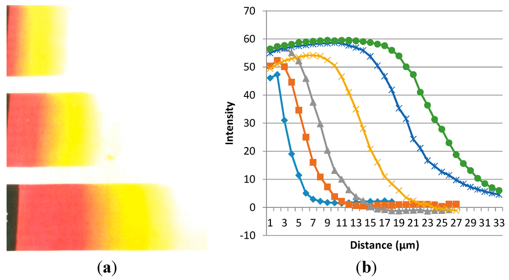
Figure 7.
(a) PAT diffusion profiles into EVA layers at different time intervals; (b) The diffusion frontier moves with time. Curves from left to right are for 30, 45, 75, 122, 180, and 240 min. The temperature for this experiment was 140 °C and the magnification of the optical microscope picture is 100×.
Using the data from Figure 7b we then evaluated the diffusion coefficient using the Equation (4):
where X is the diffusion distance in the selected direction at a time t. D is the diffusion coefficient, with a unit of cm2/s and the diffusion coefficients obtained after heating to the three different temperatures are shown in Figure 8. The fastest diffusion = largest diffusion coefficient values occur at highest temperatures and at smallest PDDT concentrations. At high temperatures the diffusion profiles become narrow and the meaning of the selection of the intensity point becomes smaller. Diffusion is clearly stabilized at longer times/distances. The largest diffusion coefficient at 160 °C is 8.44 × 10⁻⁷ cm2/s. The large diffusion coefficient of PDDT is an effect of the long side chains attributing the solvent-like effect as also seen in PDDT’s liquid crystal like behavior.
D = <X2>/(2t)

Figure 8.
Diffusion coefficients at different temperatures.
Figure 8.
Diffusion coefficients at different temperatures.
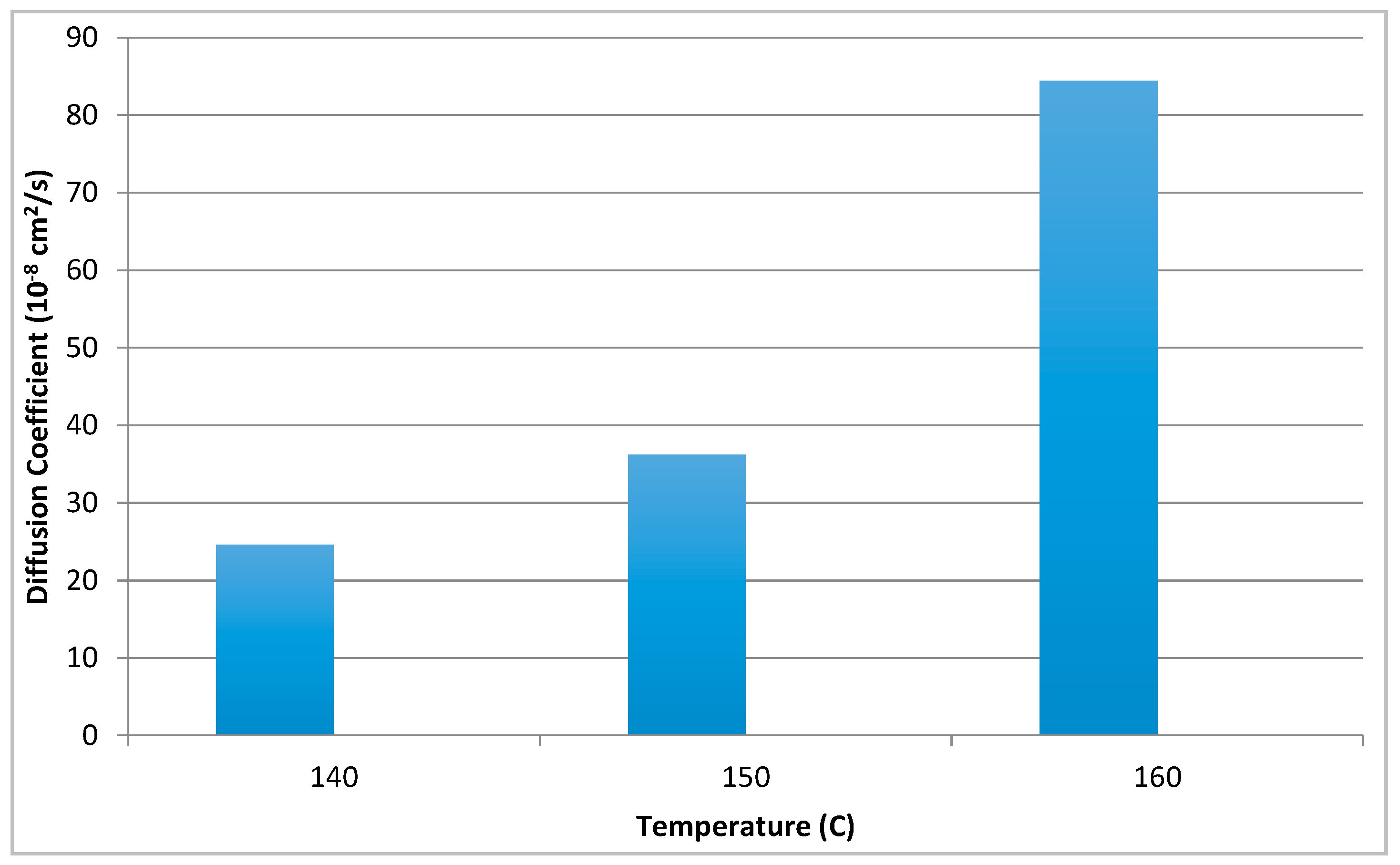
The large diffusion coefficient of PDDT is an effect of the long side chains attributing the solvent-like effect as also seen in PDDT’s liquid crystal like behavior.
4. Materials and Methods
4.1. Monomer Preparation
Monomer was made in two different batches (A and B). First the Grignard-reagent was made, the amounts of reagents are shown in Table 1. Dry ether and vacuum dried magnesium were placed in a 3-neck flask (condenser, nitrogen-atmosphere and magnetic stirring). The N2-atmosphere is necessary because the Grignard-reagent is sensitive to humidity and oxygen. Stirring was started and a few crystals of iodine was added. After that 3-bromododecane was added slowly, drop by drop, because of the exothermic reaction. The reaction was started by a little warming with a hair dryer. The adding of 3-bromododecane was controlled so that the mixture was refluxed evenly. After all alkylbromide was added the flask was placed in an oil bath and the reflux was maintained for two hours at 50 °C. Then the reaction vessel was left to cool down to room temperature.

Table 1.
Amounts of used reagents when the Grignard reagent for monomer batches A and B was made.
| Reagent | Monomer Batch A | Monomer Batch B |
|---|---|---|
| Dry ether | 200 mL | 400 mL |
| Magnesium | 13 g (0.53 mol) | 26 g (1.07 mol) |
| Iodine | Few crystals | Few crystals |
| 3-bromododecane | 54.96 g (0.22 mol) | 119.59 (0.48 mol) |
To determine the concentration of the Grignard-reagent, a sample of 10 mL was taken and put in 150 mL of deionized water. And 2–3 drops of phenolphthalein (0.5%) was added, so that the color turned to violet. Then 0.2044 M HCl-solution was added until the color disappeared and additionally 10 mL. After that the mixture was titrated with 0.202 M NaOH-solution, so that the color came back. After titration the concentration was calculated as follows:
where c = concentration, V = volume.
C (G-reagent) = [c(HCl)·V(HCl) − c(NaOH)·V(NaOH)]/V(sample)
The concentration of both Grignard reagents is shown in Table 2.
The volume of G-reagent was measured and it was transferred to another 3-neck flask consisting of the same equipment as the previous one. The amounts of needed 3-bromothiophene and 1,3-[bis(diphenylphosphino)propane]nickel(II)chloride were calculated from Equation (6):
where D = the amount of 3-bromothiophene (g),
where E = the amount of catalyst (1,3-[bis(diphenylphosphino)propane]nickel(II)-chloride).
D = c(G-reagent)·V(G-reagent) × 0.078
E = 0.0087D
The amounts of reagents are shown in Table 2.
Table 2.
The amounts of used reagents in monomer batches A and B.
| Reagent | Monomer Batch A | Monomer Batch B |
|---|---|---|
| G-reagent | 192 mL | 392 mL |
| C (G-reagent) | 0.840 mol/L | 0.977 mol/L |
| 3-bromothiophene | 12.58 g | 30.05 g |
| Catalyst | 0.11 g | 0. 26 g |
The catalyst was placed in the reaction vessel with G-reagent and the adding of 3-bromothiophene was started slowly, drop by drop and the vessel was heated a little with the hair dryer to start the reaction. After the reaction started the adding was controlled so that the reflux was complete. After all 3-bromothiophene was added, the reaction vessel was moved into the oil bath and warming was started. The mixture was left to reflux for three hours at 50 °C. Then the mixture was let to cool down to room temperature and it was washed in a funnel three times with deionized water, three times with saturated Na2CO3-solution and finally three times with deionized water. The yellow solution containing the monomer was dried with CaCl2 overnight. And then the ether was evaporated with rotavapor.
After evaporation the mixtures were combined and distilled under reduced pressure. Seven different fractions were obtained at different pressures and temperatures. The last two fractions had the right boiling point and were analyzed with 1H-NMR (GN-300 NMR, General Electric, Inc., Fairfield, CT, USA). They both were pure monomer (3-dodecylthiophene).
4.2. Polymerization of 3DDT
Both pure monomer fractions were polymerized separately. The fraction number seven was polymerized first. A 3-neck flask with reflux and nitrogen atmosphere was put into an ice bath. 600 mL of chloroform and 46.5 g of ferrichloride were placed in the flask. To reach the low temperature (+5 °C) the mixture was first stirred about 15 min and after that during 30 min 18.3 g of 3-dodecylthiophene was added into the mixture. Stirring was continued an additional four hours and the ice bath was removed after 3.5 h. The obtained viscose, black mixture was poured into a solution of methanol and HCl (1000 mL:50 mL). During precipitation the mixture was stirred with a glass rod. The black precipitate was filtrated and washed with water and methanol. The precipitate and 1100 mL of chloroform were put in a flask covered with aluminum foil and stirred overnight. Next day the reddish solution was washed twice with deionized water, once with solution of NH4·OH and water (1:9) and finally twice with water. The orange-red solution was precipitated in a solution of 2500 mL of methanol and 75 mL of HCl; it was let to precipitate overnight. After that the mixture was filtrated and the precipitate was washed with water and methanol. P3DDT was dried under vacuum in room temperature. After drying the polymers from both batches, they were dissolved in 1000 mL of chloroform and stirred over weekend. Then the polymer-solution was poured in 2500 mL of methanol and it was let to precipitate in refrigerator overnight. The next day the mixture was filtrated and the polymer was dried under vacuum at room temperature for three days. The yield of the polymer was about 22 g (64%).
4.3. Purification of P3DDTs
The polythiophene obtained from the batch one (P3DDT I) was used without further purification. The second polymer (P3DDT II) was purified several times and the iron was tested from the washing-solutions with KMnO4-solution, which forms a red solution in the presence of iron.
P3DDT II was first dissolved in chloroform (about 1 wt% solution). The solution was let to stir overnight. To obtain a clear solution it has to be heated a little, but the temperature was kept at ~40 °C and only for a few minutes. After dissolving the solution was filtrated and then the precipitation was done by pouring methanol in the solution so that the color changed from orange to brown and so much that the color did not change any more after adding methanol. The polymer was let to precipitate overnight in refrigerator before filtration. Then the iron was tested from the filtrate and the precipitate was dried under vacuum in room temperature overnight. This purification was done so many times, that no iron could be noticed from the filtrate.
4.4. Gel Permeation Cromatography (GPC)
The GPC of EVA20 was done in Neste Company, Porvoo, Finland. Its weight average molecular weight (Mw) is 224,403, number-average molecular weight (Mn) is 18,040, and molecular weight distribution (d) is 12.44.
4.5. Differential Scanning Calorimetry
The temperature profile for P3DDT thermal analysis with Perkin-Elmer DSC-7 (Waltham, MA, USA) was following: the starting temperature was −60 °C and it was kept there for 15 min, then the sample was heated up to 200 °C with 10 °C/min heating rate and left to stay there for 3 min, after cooling down (10 °C/min) to −60 °C, the second heating was done like the first one. The melting point for P3DDTs was taken from the middle of the double peak; for P3DDT I it was ~138 °C and for P3DDT II 130 °C.
4.6. Infrared Spectroscopy
The IR-spectra obtained with the Perkin-Elmer 1600 series FTIR the spectra was scanned 16 times with the resolution was 2 cm−1. The peak positions were compared with those found in literature [34] and the comparison is expressed in Table 3.
Table 3.
The IR-spectra of P3DDTs compared to the values in literature.
| Peak # | Mode | P3DDT I | PDDT II | Reference [34] |
|---|---|---|---|---|
| 1 | CH2 rocking band | 721 | 721 | 725 |
| 2 | C–H out-of-plane vibrations | 823 | 825 | 819 |
| 3 | Bending of the dodecyl group | 1,377 | 1,376 | 1,377 |
| 4 | Stretching of the 2,5 substituted thiophene ring | – | – | 1,440 |
| 5 | The same as #4 | 1,465 | 1,465 | 1,454 |
| 6 | The same as #4 | 1,511 | 1,511 | 1,509 |
| 7 | Stretching of the 3-dodecyl group | 2,852 | 2,853 | 2,853 |
| 8 | The same as #7 | 2,955 | 2,954 | 2,954 |
| 9 | Cb–H stretching | 3,057 | 3,056 | 3,058 |
4.7. UV-Visible Spectroscopy
The UV results were obtained by Varian DMS 100S UV-Visible spectrophotometer (Palo Alto, CA, USA) using 200 nm/min scanning rate and wavelength range from 300 nm to 700 nm. The absorption maximum at 500 nm and the shoulder positions at 560 nm and 600 nm were same for both thiophenes.
4.8. Film Preparation
1 wt% solution in chloroform was done from each of the polymer. The solution were stirred at least three days or so long, that a clear solution was obtained. The EVA-solutions were warmed a little and then cooled down before casting. The P3DDT-solution bottles were covered with aluminum foil, because P3DDT in chloroform is very sensitive to light.
After the clear solutions were obtained the films were casted on Petri-dishes by pouring a certain amount of polymer-solution in a Petri-dish and then evaporating the chloroform first in fume hood and finally in vacuum at least 24 h. The P3DDT films were casted in a dark room with light.
After evaporation the films were peeled off the Petri-dishes by pouring deionized water on the films. Then the films were dried under vacuum 24 h.
After drying the samples were made. First a small piece (~10 mm × 10 mm) of the matrix film (EVA) was cut with razor blade and placed on a microslide and then even smaller piece of P3DDT (~2 mm × 10 mm), which was cut either with razor blade or in liquid nitrogen, was placed on the top of the matrix polymer. In Figure 9 is a schematic illustration of the bilayer preparation. During the work it was noticed that the cover has an effect on the diffusion and that is why some of the samples were done without cover glass.
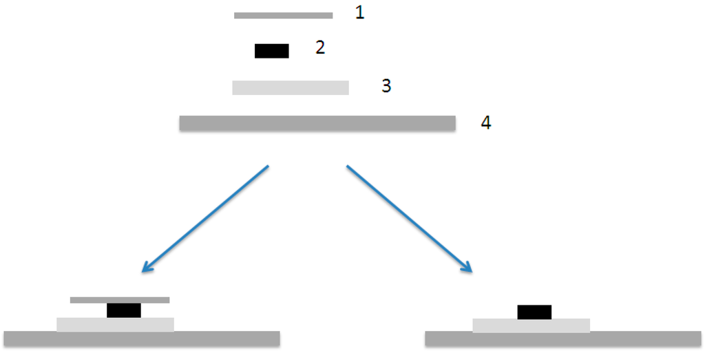
Figure 9.
A schematic illustration of the bilayer preparation. (1) Cover glass, (2) P3DDT-film, (3) matrix (EVA)-film and (4) microslide. On the left sample with cover glass and on the right without cover.
Figure 9.
A schematic illustration of the bilayer preparation. (1) Cover glass, (2) P3DDT-film, (3) matrix (EVA)-film and (4) microslide. On the left sample with cover glass and on the right without cover.

The cutting of P3DDT-films in liquid nitrogen was done so that a slice of the film was placed between two microslides with a small piece of film was outside. Then the “three-layer” sandwich was put in liquid nitrogen for a while and after that the small piece of film was hit with another microslide and a nice film slice was obtained.
5. Conclusions
Electrically conducting polymers, such as alkylated polythiophenes (PAT), can form a thermodynamically miscible blend with a thermoplastic insulating polymers under certain mixing conditions, mainly depending on the molecular control parameters: the degree of polymerization, statistical segment length and the Flory-Huggins interaction parameter. The alkyl group behave in a liquid-like manner promoting liquid crystallinity, improved entropy, and also limited interactions. In this manuscript we evaluate the mixing and demixing processes of the PATs: the spinodal decomposition from the miscible state and the interdiffusion of the separated components at elevated temperatures reveal comparable diffusion behavior and the possibility of controlling percolate conditions with the thermodynamic parameters. The interesting relation with the morphology and phase separation kinetics was observed importantly as several studies [35,36,37,38] have evaluated the bicontinuity only based on morphology from solvent cast blend samples.
Author Contributions
Jukka Seppälä and Kalle Levon designed the research; Antti Takala, Päivi Takala and Kalle Levon conducted the experimentation and wrote the manuscript.
Conflicts of Interest
The authors declare no conflict of interest.
References
- Chiang, C.K.; Druy, M.A.; Gau, S.C.; Heeger, A.J.; Louis, E.J.; MacDiarmid, A.G.; Park, Y.W.; Shirakawa, H. Synthesis of highly conducting films of derivatives of polyacetylene, (CH)x. J. Am. Chem. Soc. 1978, 100, 1013–1015. [Google Scholar]
- Chen, D.; Nakahara, A.; Wei, D.; Nordlund, D.; Russell, T.P. P3HT/PCBM bulk heterojunction organic photovoltaics: Correlating efficiency and morphology. Nanoletters 2010, 11, 561–567. [Google Scholar]
- Nasybulin, E.; Wei, S.; Cox, M.; Kymissis, I.; Levon, K. Morphological and spectroscopic studies of electrochemically deposited poly(3,4-ethylenedioxythiophene) (PEDOT) hole extraction layer for organic photovoltaic device (OPVd) fabrication. J. Phys. Chem. C 2011, 115, 4307–4314. [Google Scholar]
- Nasybulin, E.; Feinstein, J.; Cox, M.; Kymissis, I.; Levon, K. Electrochemically prepared polymer solar cell by three-layer deposition of poly(3,4-ethylenedioxythiophene)/poly(2,2'-bithiophene)/fullerene (PEDOT/PBT/C60). Polymer 2011, 52, 3627–3632. [Google Scholar]
- Nasybulin, E.; Cox, M.; Kymissis, I.; Levon, K. Electrochemical codeposition of poly(thieno[3,2-bithiophene) and fullerene: An approach bulk heterojunction organic photovoltaic device (OPVd). Synth. Met. 2012, 162, 10–17. [Google Scholar]
- Nasybulin, E.; de Albuquerque, I.; Levon, K. Electrochemical synthesis of oligothiophenes by radical termination of the growing macromolecular chain. Electrochim. Acta 2012, 63, 341–345. [Google Scholar]
- Levon, K.; Ho, K.-S.; Laakso, J.; Mao, J.; Zheng, W.-Y. Phase behavior of undoped poly(3-alkyl thiophene) with ethylene-co-vinylacetates. A solvatochromatic transition in the solid state. Synth. Met. 1993, 55–57, 3591–3596. [Google Scholar]
- Levon, K.; Chu, E.; Ho, K.-S.; Kwei, T.K.; Mao, J.; Zheng, W.-Y.; Laakso, J. Miscibility studies of poly(3-octylthiophene)/poly(ethylene-co-vinylacetate) blends with a solvatochromatic shift in the solid state. J. Polym. Sci. B 1995, 33, 537–545. [Google Scholar]
- Levon, K.; Margolina, A.; Patashinky, A.Z. Multiple percolation in conducting polymer blends. Macromolecules 1993, 26, 4061–4063. [Google Scholar]
- Reich, S. Percolation characteristics of spinodal phase separation in polymer blends. Phys. Lett. 1986, 114A, 90–94. [Google Scholar]
- Cahn, J.W. Phase separation by spinodal decomposition in isotropic systems. J. Chem. Phys. 1965, 42, 93–99. [Google Scholar]
- Cahn, J.W. Spinodal decomposition. Transac. Metall. Soc. AIME 1968, 242, 166–180. [Google Scholar]
- Hashimoto, T.; Kumaki, J.; Kawai, H. Time resolved light scattering studies on kinetics of phase separation and phase dissolution of polymer blends. 1. Kinetics of phase separation of a binary mixture of polystyrene and poly-(vinylmethylether). Macromolecules 1983, 16, 641–648. [Google Scholar] [CrossRef]
- Nojima, S.; Tsutsumi, K.; Nose, T. Phase separation process in polymer systems. I. Light scattering studies on a polystyrene and poly(methylphenylsiloxane) mixture. Polym. J. 1982, 14, 225–232. [Google Scholar]
- Nojima, S.; Ohyama, Y.; Yamaguchi, M.; Nose, T. Phase separation process in polymer systems. III. Decomposition in the critical mixture of polystyrene and poly(methylphenylsiloxane) and scaling analysis. Polym. J. 1982, 14, 907–912. [Google Scholar]
- Snyder, H.; Meakin, P.; Reich, S. Dynamical aspects of phase separation in polymer blends. Macromolecules 1983, 16, 757–762. [Google Scholar]
- Izumitani, T.; Hashimoto, T. Slow spinodal decomposition in binary liquid mixtures of polymers. J. Chem. Phys. 1985, 83, 3694–3701. [Google Scholar]
- Hashimoto, T.; Itakura, M.; Shimidzu, N. Late stage spinodal decomposition of a polymer mixture. II. Scaling analyses on Qm(τ) and Im(τ). J. Chem. Phys. 1986, 85, 6773–6786. [Google Scholar]
- Takenaka, M.; Hashimoto, T.; Izumitani, T. Slow spinodal decomposition in binary liquid mixtures of polymers. 2. Effects of molecular weight and transport mechanism. Macromolecules 1987, 20, 2257–2264. [Google Scholar] [CrossRef]
- Yang, H.; Shibayama, M.; Stein, S.S.; Shimizu, N.; Hashimoto, T. Deuteration effects on the miscibility and phase separation kinetics of polymer blends. Macromolecules 1986, 19, 1667–1674. [Google Scholar]
- Inaba, N.; Sato, K.; Suzuki, S.; Hashimoto, T. Morphology control of binary polymer mixture by spinodal decomposition and crystallization. 1. Principle of method and premilinary results on PP/EPR. Macromolecules 1986, 19, 1690–1695. [Google Scholar] [CrossRef]
- Nakai, A.; Shiwaku, T.; Hasegawa, H.; Hashimoto, T. Spinodal decomposition of polymer mixtures with a thermotropic liquid crystalline polymer as one component. Macromolecules 1986, 19, 3008–3010. [Google Scholar]
- Inaba, N.; Yamada, T.; Suzuki, S.; Hashimoto, T. Morphology control of binary polymer mixture by spinodal decomposition and crystallization. 2. Further studies on polypropylene ethylene-propylene random copolymer. Macromolecules 1988, 21, 407–414. [Google Scholar] [CrossRef]
- Hashimoto, T.; Izumitani, T.; Takenaka, M. Homogenization of immiscible rubber/rubber polymer mixtures by uniaxial compression. Macromolecules 1989, 22, 2293–2302. [Google Scholar]
- Hashimoto, T.; Sasaki, K.; Kawai, H. Time resolved light scattering studies on kinetics of phase separation and phase dissolution of polymer blends. 2. Phase separation of ternary mixtures of polymer A, polymer B, and solvent. Macromolecules 1984, 17, 2812–2818. [Google Scholar] [CrossRef]
- Sasaki, K.; Hashimoto, T. Time resolved light scattering studies on kinetics of phase separation and phase dissolution of polymer blends. 3. Spinodal decomposition of ternary mixtures of polymer A, polymer B, and solvent. Macromolecules 1984, 17, 2818–2825. [Google Scholar] [CrossRef]
- Inoue, T.; Ougizawa, T.; Yasuda, Y.; Miyasaka, K. Development of modulated structure during solution casting of polymer blends. Macromolecules 1985, 18, 57–63. [Google Scholar]
- Inoue, T.; Ougizawa, T. Characterization of phase behavior in polymer blends by light scattering. J. Macromol. Sci. Chem. 1989, 26, 147–173. [Google Scholar]
- Nishi, T.; Wang, T.T.; Kwei, T.K. Thermally induced phase separation behavior of compatible polymer mixtures. Macromolecules 1975, 8, 227–234. [Google Scholar]
- Nojima, S.; Shiroshita, K.; Nose, T. Phase separation process in polymer systems. II. Microscopic studies on a polystyrene and diisodecylphthalate mixture. Polym. J. 1982, 14, 289–294. [Google Scholar]
- Han, C.C.; Okada, M.; Muroga, Y.; Mccrackin, F.L.; Bauer, B.J.; Tran-Cong, Q. Static and kinetic studies of polystyrene/poly(vinylmethylether) blends. Polym. Eng. Sci. 1986, 26, 3–8. [Google Scholar]
- Russell, T.P.; Hadziioannou, G.; Warburton, W.K. Phase separation in low molecular weight polymer mixtures. Macromolecules 1985, 18, 78–83. [Google Scholar]
- Jabbari, E.; Peppas, N.A. Use of ATR-FTIR to study interdiffusion in polystyrene and poly(vinyl methyl ether). Macromolecules 1993, 26, 2175–2186. [Google Scholar]
- Inganäs, O.; Salaneck, W.R.; Österholm, J.-E.; Laakso, J. Thermochromic and solvatochromic effects in poly(3-hexylthiophene). Synth. Met. 1988, 22, 395–406. [Google Scholar]
- Wang, J.Z.; Zheng, Z.H.; Li, H.W.; Huck, W.T.S.; Sirringhaus, H. Dewetting of conducting polymer inkjet droplets on patterned surfaces. Nat. Mater. 2004, 3, 171–176. [Google Scholar]
- Asadi, K.; Wondergem, H.J.; Moghaddam, R.S.; McNeill, C.R.; Stingelin, N.; Noheda, B.; Blom, P.W.M.; de Leeuw, D.M. Spinodal decomposition of blends of semiconducting and ferroelectric polymers. Adv. Funct. Mater. 2011, 21, 1887–1894. [Google Scholar]
- Haberko, J.; Raczkowska, J.; Bernasik, A.; Rysz, H.; Nocun, M.; Nizioł, J.; Łuz ̇ny, W.; Budkowski, A. Conductivity of thin polymer films containing polyaniline. Mol. Cryst. Liq. Cryst. 2008, 485, 796–803. [Google Scholar]
- Mezzenga, R.; Ruokolainen, J.; Fredrickson, G.H.; Kramer, E.J.; Moses, D.; Heeger, A.J.; Ikkala, O. Templating organic semiconductors via self-assembly of polymer colloids. Science 2003, 299, 1872–1874. [Google Scholar] [CrossRef] [PubMed]
© 2015 by the authors; licensee MDPI, Basel, Switzerland. This article is an open access article distributed under the terms and conditions of the Creative Commons Attribution license (http://creativecommons.org/licenses/by/4.0/).