3.1. Mathematical Relationship among the Three Equations
The WLF equation was first proposed by Williams et al. to describe the temperature dependence of relaxation mechanisms in amorphous polymers [
2]. It is usually expressed in the following form:
in which
αT is the shift factor, the ratio of relaxation times at temperatures
T and
Ts, respectively.
Ts is the reference temperature, and
C1,
C2 are empirical constants.
C1 = 17.44 and
C2 = 51.6 K are applicable to most amorphous polymers provided
Tg is chosen as
Ts. A concept, the so-called cooperatively rearranging region introduced by the Adam–Gibbs theory [
3] and the free-volume theory [
1], has provided the theoretical rationalization for the WLF equation. Another equation equivalent to the WLF function called the VFTH equation is given as [
4,
5]:
where
τ is the relaxation time at
T,
τ0 is a pre-exponential factor,
B is a numerical constant and
T∞ is the so-called Vogel temperature. Based on the definition of the shift factor,
αT is the ratio of two relaxation times, which can be expressed as Equation (2), and rearranging the resulting formula algebraically as the WLF form yields [
27] (the detailed mathematical derivation is provided in the
Supporting Information):
According to the Adam–Gibbs theory,
T∞ is the temperature at which conformational entropy induced by segment motion vanishes and is about 50~60 K below the
Tg for most polymers [
3]. This fact is consistent with the empirical value of the WLF equation, i.e.,
C2 = 51.6 K in the case of
Ts =
Tg. Moreover, for the WLF and VFTH equations, there are the same temperatures at which the relaxation time is infinity, i.e.,
TWLF =
TVFTH =
T∞ (
TWLF =
Ts −
C2,
C2 =
Ts −
T∞), which accords with the Adam–Gibbs theory.
On the other hand, it is well known that secondary relaxations and terminal flow follow an Arrhenius behavior written as:
in which
Ea is the activation energy of relaxation and
R is the gas constant. Moreover,
Ea is the temperature independent activation energy in the Arrhenius form [
3]. However, as for real polymers, approaching the glass transition, the apparent activation energy of relaxation will increase significantly [
19]. This is the obstacle in essence hindering the application of the Arrhenius equation to glass-forming liquids. Regardless, mathematically, the Arrhenius form is the limit equation of the VFTH form provided
T∞ = 0. Consequently, ignoring the physical meaning of
T∞, the VFTH and WLF form may be universal for glass-forming liquids and terminal flow of polymers. The rationality of
T∞ = 0 for the application of the VFTH or WLF equation at high temperatures will be discussed in more detail later.
Introducing relaxation times of the Arrhenius form into the shift factor, the resulting formula rearranged algebraically as the WLF form can be written as (the detailed mathematical derivation is provided in the
Supporting Information):
Introducing two new parameters
and
,
Then, a developed WLF (DWLF) equation derived from the Arrhenius form can be obtained:
Certainly, Equation (9) is applicable to terminal flow of polymers at high temperatures as Equation (5), at least while
= 0.434
Ea/
RTs,
=
Ts. However, the doubt is whether there are rational values for
and
that are suitable for glass-forming liquids and terminal flow simultaneously. For this purpose, the apparent activation energy of Equation (9) should meet two requirements: (i) it decreases strongly with increasing temperature nearby the glass transition; (ii) it tends to be a temperature independent value at high temperatures far away from the glass transition. For the WLF equation, apparent activation energy can be calculated formally as [
1,
27]:
Analogously, the apparent activation energy of Equation (9) can be written as:
In order to meet the two requirements above, we have:
From the calculation of the two inequalities above, the criterion for the universality of Equation (9) can be obtained:
Consequently, Equation (9) may be universal while the criterion above (Inequality (14)) is met. However, it should be pointed out that when = Ts, Equation (9) will evolve into the Arrhenius equation according to Equation (6), and the criterion (Inequality (14)) is a necessary, but not a sufficient condition for the universality of Equation (9).
3.2. Application of the DWLF Equation for Viscoelastic Behavior of Pure Polymers at High Temperatures
As mentioned above, the DWLF equation may be applied at high temperatures where the Arrhenius equation is traditionally employed. Here, the viscoelastic properties of various pure polymers (crystalline and amorphous polymer) and polymer blends (amorphous/amorphous blend and crystalline/amorphous blend) were investigated.
Figure 1 gives the master curve by horizontal shifting of the frequency (
ω) dependence of the dynamic storage modulus (
G′) and dynamic loss modulus (
G″) for pure
iPP at temperatures from 424 to 525 K. It is found that all curves obtained at different temperatures can superpose together and then form a satisfactory master curve by horizontal shifting. This result indicates that the TTS principle can be applicable for
iPP at high temperatures.
However, it should be pointed out that from the theory of free volume, the WLF equation is only applicable for amorphous polymers at the temperature range of
Tg ~
Tg + 100 K [
1,
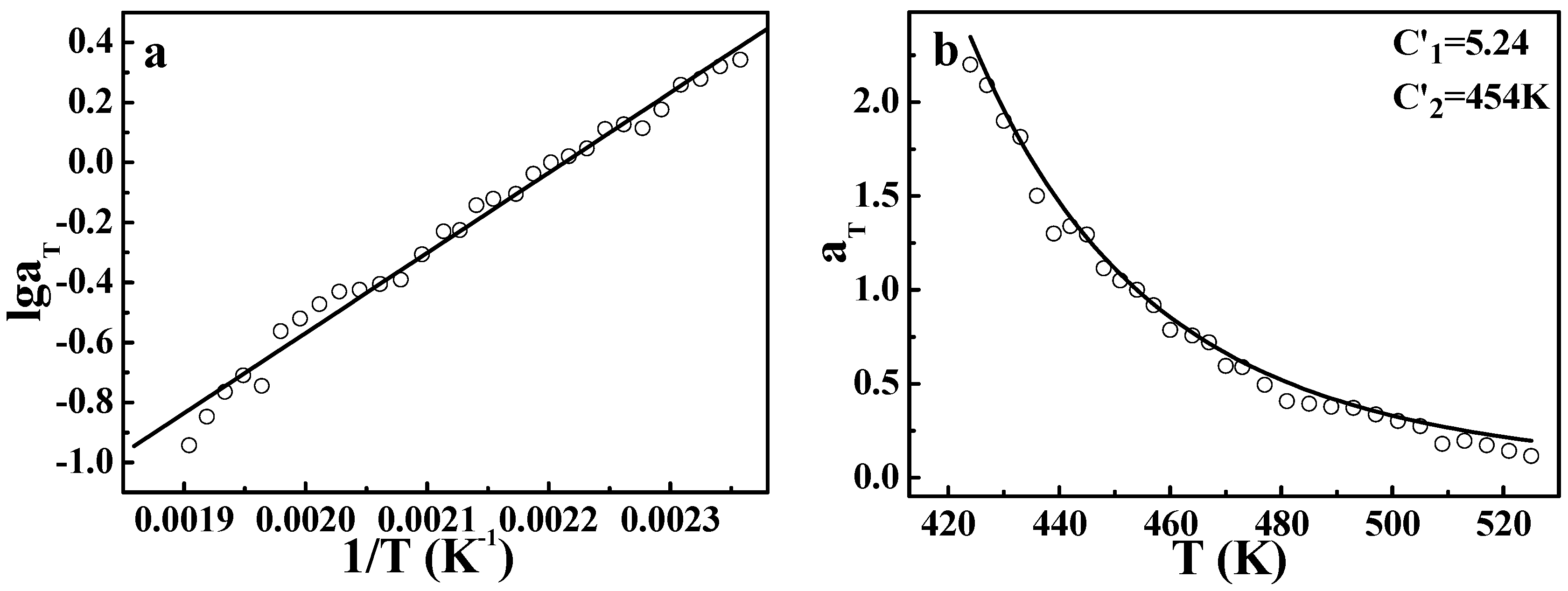
2], since the crystalline phase will certainly restrict the expansion of free volume and change the linear dependence of free volume on temperature. While in the molten state, the limitation of the crystalline phase vanishes, the equation of the WLF form may be applicable again. Based on this understanding and the discussion above, both the Arrhenius equation and the DWLF equation are used to describe TTS of
iPP, as shown in
Figure 2. It is to be expected that both = equations can describe TTS of
iPP well at high temperatures. Here,
Ts = 454 K is chosen as the reference temperature, and the two parameters of the DWLF form are
C1′ = 5.24 and
C2′ = 454 K, respectively. The extreme equivalence of
C2′ to
Ts indicates that this result is logical according to the criterion above (Inequality (14)). However, the values of the two parameters deviate from the empirical values of the WLF equation, suggesting that the apparent activation energies of the viscoelastic behavior for different polymers at high temperatures vary widely and may be correlated with a specific chemical structure [
28]. This viewpoint is also supported by Williams’ results [
2] that the curves log
αT ~ (
T −
Ts) no longer overlap for different polymers at high temperatures. In that case,
C1′ and
C2′ will deviate from the empirical values. These results show that the viscoelastic behavior of
iPP, a typical crystalline polymer, follows the TTS principle and could be described by the DWLF equation in the molten state, in spite of the deviation from empirical values for
C1′ and
C2′.
It should be reasonable that the choice of reference temperature is quite arbitrary according to the knowledge of the traditional WLF equation.
Table 1 gives the two parameters at different reference temperatures. Additionally, the goodness of fit (GOF) calculated from:
was used to evaluate the consistency between measured value
yi and calculated value
yi′ from the DWLF equation.
It is clearly seen that for all reference temperatures investigated, the value of
C2′ is equal to that of
Ts, meaning that the choice of reference temperature can be indeed quite arbitrary. Moreover, the results of the viscoelastic behavior described by the DWLF equation at other reference temperatures are also perfect (seen in the
Supporting Information, Figure S1). Considering that the glass transition temperature of
iPP is about 288 K (seen in the
Supporting Information, Figure S2), the temperature here is much higher than
Tg + 100 K, indicating that the application of the DWLF equation at high temperatures is feasible. Furthermore, the apparent activation energy of viscoelastic behavior can be calculated from the Arrhenius equation, i.e., ∆
Ea = 51.2 kJ/mol, while that obtained by using the data in
Table 1 with the DWLF equation according to Equation (7) is ♦
Ea-WLF = 48.1 ± 3.1 kJ/mol. These two values of apparent activation energies are approximate, confirming the effectiveness of the DWLF equation at high temperatures again.
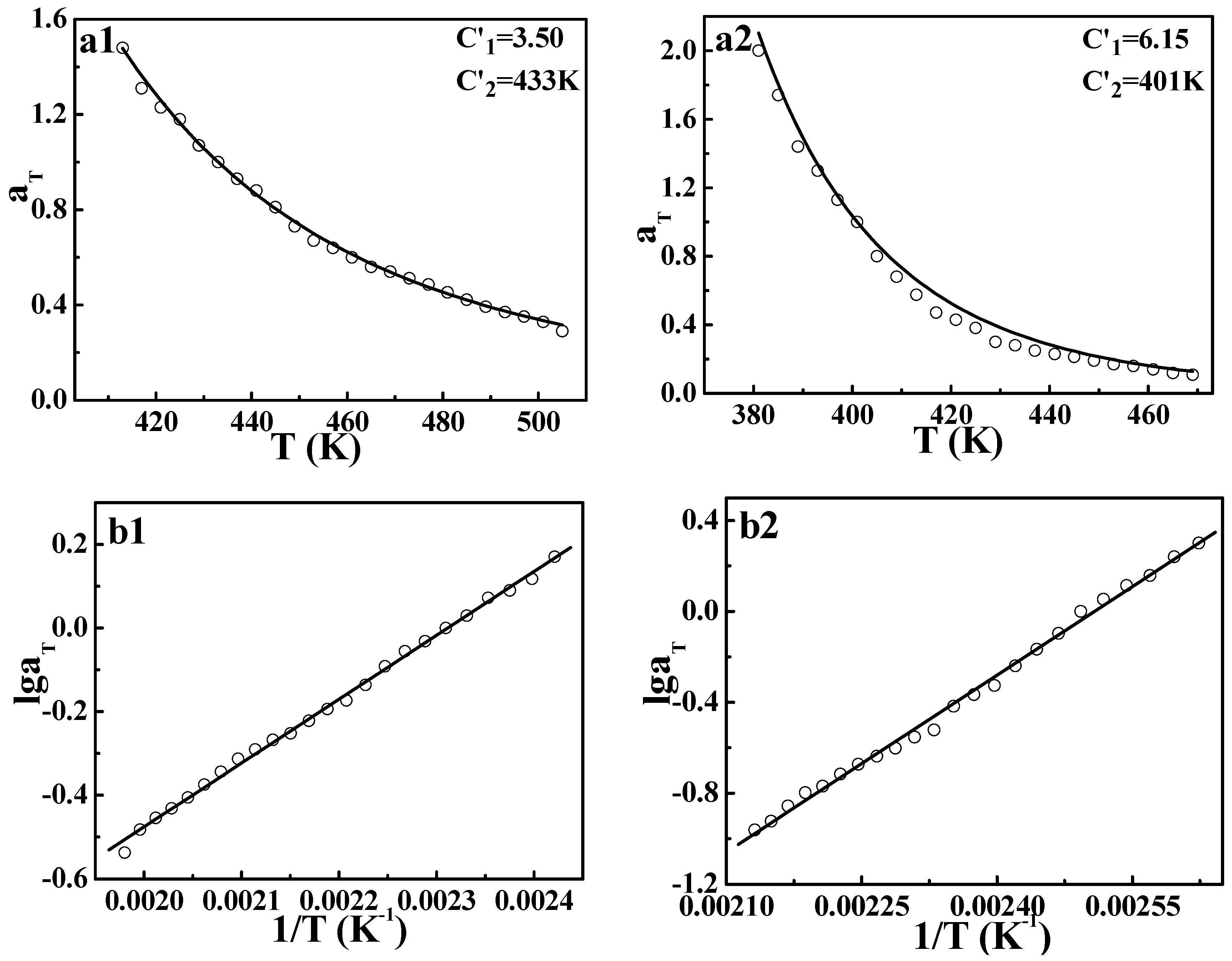
However, the application of the TTS principle to viscoelastic behavior for crystalline polymers is still rarely reported. In order to further explore the validity of the DWLF equation, another two crystalline polymers, i.e., HDPE and LDPE, were also investigated. The master curves of HDPE and LDPE are displayed in
Figure 3. Similar to the case of
iPP, both HDPE and LDPE show a good overlapping curve. Moreover, the temperature dependences of shift factors described by the DWLF equation and the Arrhenius equation for each polymer are shown in
Figure 4. It is found that as a whole, the DWLF equation can describe the relaxation behavior well for them in the molten state similar to the Arrhenius form. It is noted that the fitting curve of the DWLF equation deviates from the experimental data for LDPE at a temperature ranging from 400 to 440 K, as shown in
Figure 4(a2). It may be ascribed to the existence of the abundantly branched structure in LDPE, which may lead to some additional relaxation. In addition, the values of parameter
C2′ are equal to the reference temperatures, respectively, according to the criterion above (Inequality (14)). At other reference temperatures, the results are also perfect. Considering the fact that both the glass transition temperatures of HDPE and LDPE are far lower than the temperature range investigated here (166 K and 158 K for
Tg of HDPE and LDPE respectively, seen in the
Supporting Information, Figure S3), it is reasonable to draw the conclusion that in the molten state, the limitation of the expansion of free volume by the crystalline phase disappears, leading to the application of the DWLF equation. From the calculation, the apparent activation energies of the viscoelastic behavior obtained by the DWLF equation and the Arrhenius form are ♦
Ea = 29.0 kJ/mol (the DWLF equation), ♦
Ea = 29.3 kJ/mol (the Arrhenius form) for HDPE, ♦
Ea = 50.0 kJ/mol (the DWLF equation) and ♦
Ea = 49.8 kJ/mol (the Arrhenius form) for LDPE, respectively. Almost the same apparent activation energy obtained by the two equations supports the universality of the DWLF equation for crystalline polymers in the molten state well.
The results of crystalline polymers above have proven that the DWLF equation at a high temperature can be equal to the Arrhenius form provided
C2′ =
Ts and can be used to describe the relaxation behavior of crystalline polymers. Consequently, it seems no obstruction for application on the amorphous polymer.
Figure 5 shows the TTS results of the viscoelastic behavior of EPR, a rubber with
Tg of 233 K (seen in the
Supporting Information). Similar to the results of crystalline polymers, the DWLF equation can describe the relaxation behavior of EPR at high temperatures far away from the glass transition range.
3.3. Application of the DWLF Equation for the Phase-Separation Behavior of Polymer Blends at High Temperatures
The discussions above have shown that the DWLF equation is applicable to describe the relaxation behavior of pure crystalline and amorphous polymers at high temperatures far above
Tg. Our previous work has also proven that the WLF-like equation can perfectly describe the phase-separation behavior of the PMMA/SAN blend investigated by SALLS within the temperature range of
Tg ~
Tg + 100 K [
13]. Considering the results above, it should be logical that the DWLF equation can also describe the phase separation behavior of polymer blends at higher temperature above
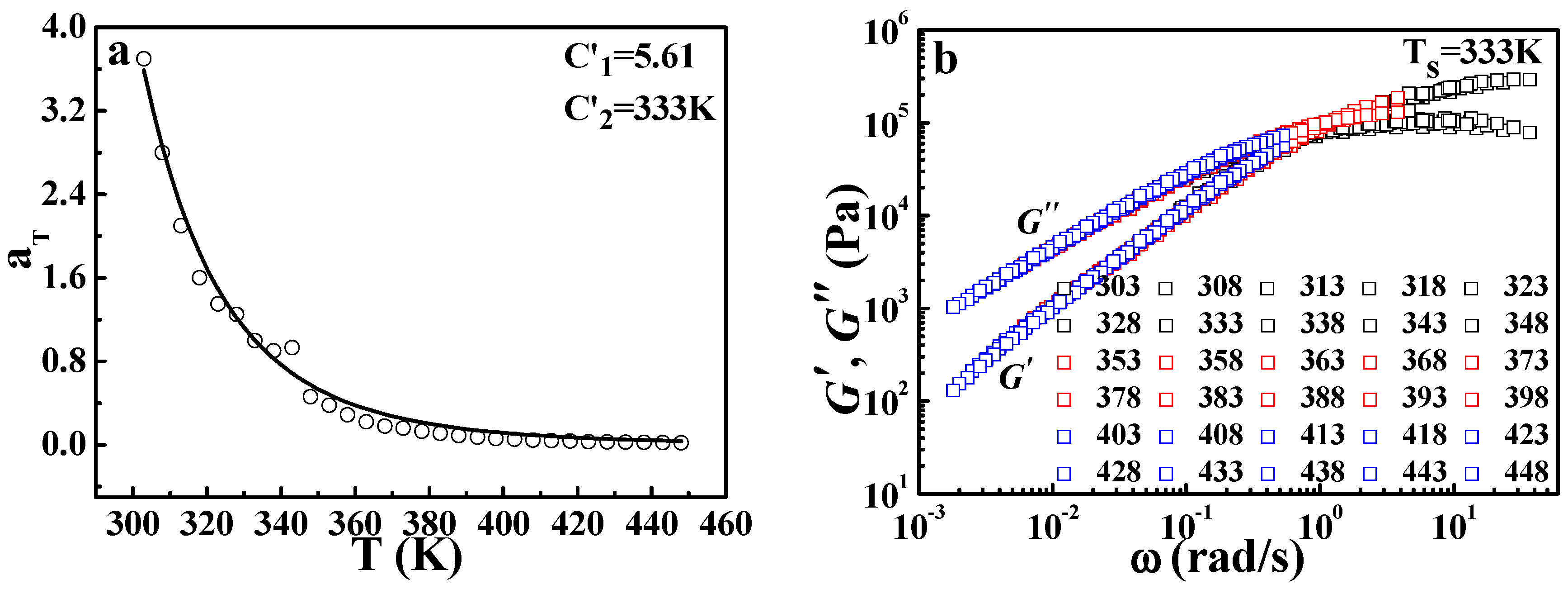
Tg + 100 K. Here, the data of the phase separation of the amorphous/amorphous polymer blend (PMMA/SMA) with a lower critical solution temperature (LCST) character, which have been described by the Arrhenius equation in our previous paper [
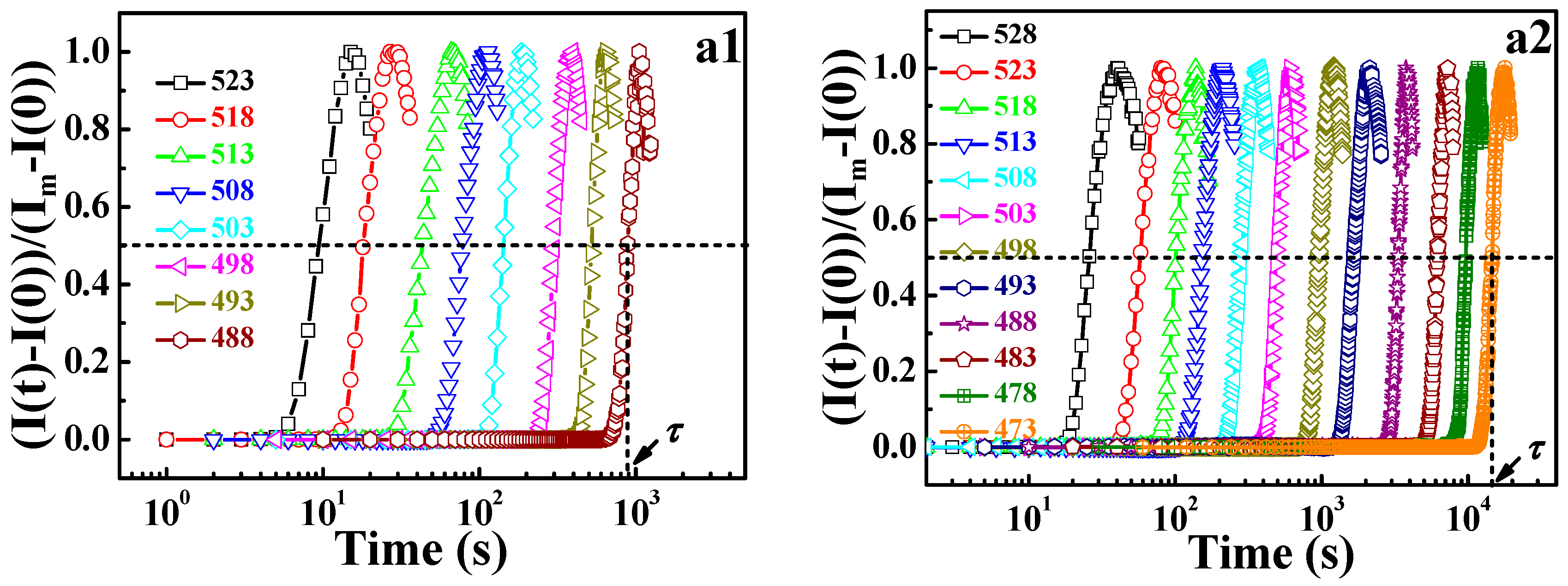
29], were re-examined. The shift factors investigated by SALLS are calculated from:
Here,
τs is the relaxation time at
Ts, and
τ is the relaxation time at which the normalized scattering intensity for different temperatures increases by the same degree, being 50% in this work, as shown in
Figure 6a. From
Figure 6b, it is seen that the DWLF equation describes the phase separation behavior of different PMMA/SMA blends well. For the two PMMA/SMA blends with different compositions, the apparent activation energies of phase separation obtained by the DWLF equation are ♦
Ea = 252.4 ± 3.0 kJ/mol and ♦
Ea = 228.8 ± 2.5 kJ/mol, respectively, which are similar to those obtained by the Arrhenius form (♦
Ea = 278.2 ± 8.4 kJ/mol and ♦
Ea = 241.5 ± 4.9 kJ/mol, respectively) [
29]. Considering the fact that liquid-liquid phase separation is a process synchronously containing disentanglement and segment motion, which depend on relaxation time and the glass transition temperatures of PMMA/SMA 60/40 and 80/20 blends, which are 385 and 378.4 K respectively [
18], the above results indicate that the DWLF equation can describe the relaxation process, i.e., rheological behavior and phase separation behavior, well at temperatures above
Tg + 100 K.
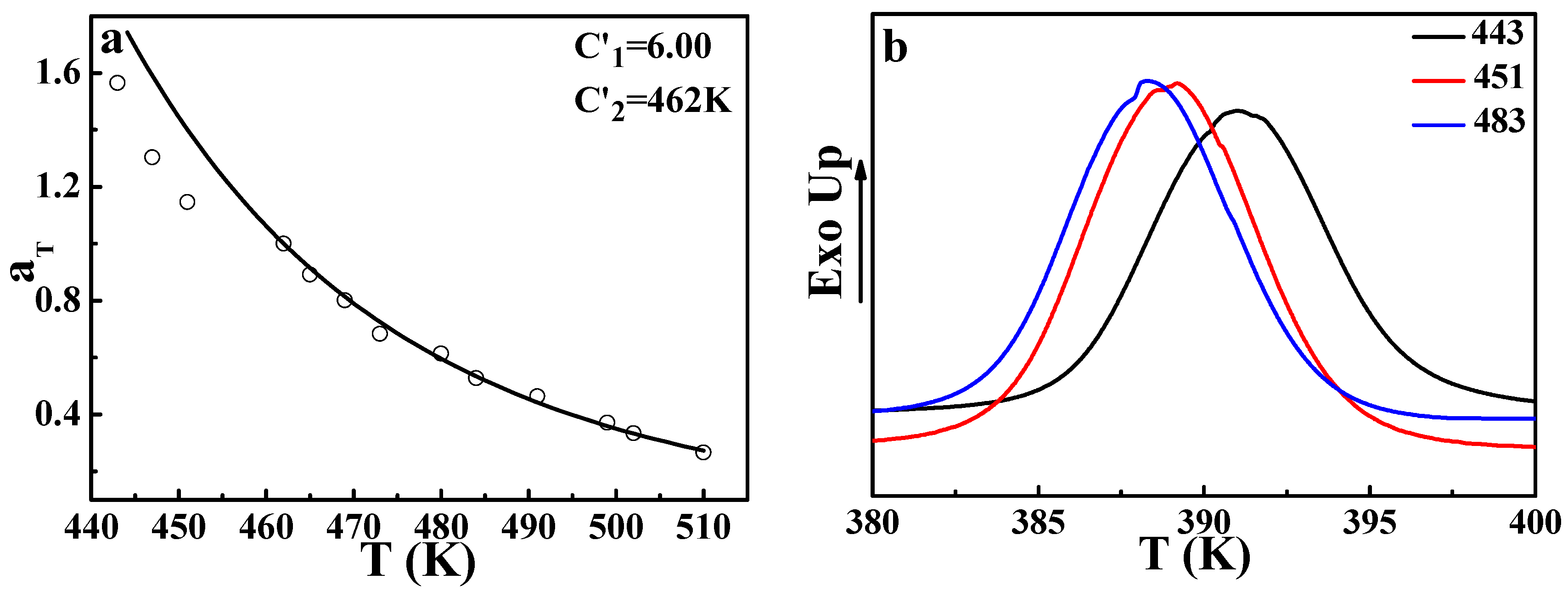
In order to further explore the validity of applying the DWLF equation to the phase separation behavior of polymer blends, a crystalline/amorphous polymer blend (
iPP/EPR) was used for investigating, as shown in
Figure 7a. It is found that at low temperatures, the experimental values of
αT deviate from the theoretical curve. However, the experimental values at high temperatures are very consistent with the DWLF curve. Considering that the equilibrium melting point of
iPP is 460 K [
30],
iPP will crystallize when the temperature is below 460 K in theory. Furthermore, it was pointed out that nucleation behavior may exist, and the lamellar structures of
iPP can survive in the melt for a long time even if the annealing temperature is above the apparent melting point,
Tm [
31]. Regardless, the final point of the melting temperature range is 448 K for
iPP (seen in the
Supporting Information). This fact means that at these temperatures, the nucleation of
iPP may happen, though the crystal growth is extremely slow at temperatures near the equilibrium melting point.
Figure 7b gives the crystallization behavior of
iPP after being annealed at different temperatures for 30 min. The increase of the crystallization temperature after being annealed at 443 K and 451 K indicates that the nucleation process indeed exists even at a temperature higher than its
Tm (439 K, seen in the
Supporting Information). It is well known that during the crystallization process, the heterogeneous components can be excluded from the crystalline phase [
32]. There is no doubt that this nucleation behavior can lead to a heterogeneous concentration fluctuation. In other words, at these temperatures, heterogeneous concentration fluctuation resulting from nucleation of
iPP could affect the phase-separation behavior. That means the existence of the nucleation of
iPP provides an additional contribution to the phase-separation, indicating that the time required for a 50% increase of the scattered light intensity becomes shorter, leading to a smaller
αT than the theoretical value. This may be the cause of the slight deviation in the melting region.
3.4. Universality of the DWLF Equation in a Wide Temperature Range
The above results indicate that the application of the DWLF equation at high temperatures where the Arrhenius equation is traditionally employed is appropriate indeed. Consequently, the universality of Equation (9) at temperatures from glass transition to very high temperatures seems reasonable. Here, due to the suitable
Tg (378 K for PS, seen in the
Supporting Information), PS was used to examine the universality of Equation (9) from
Tg to much high temperatures.
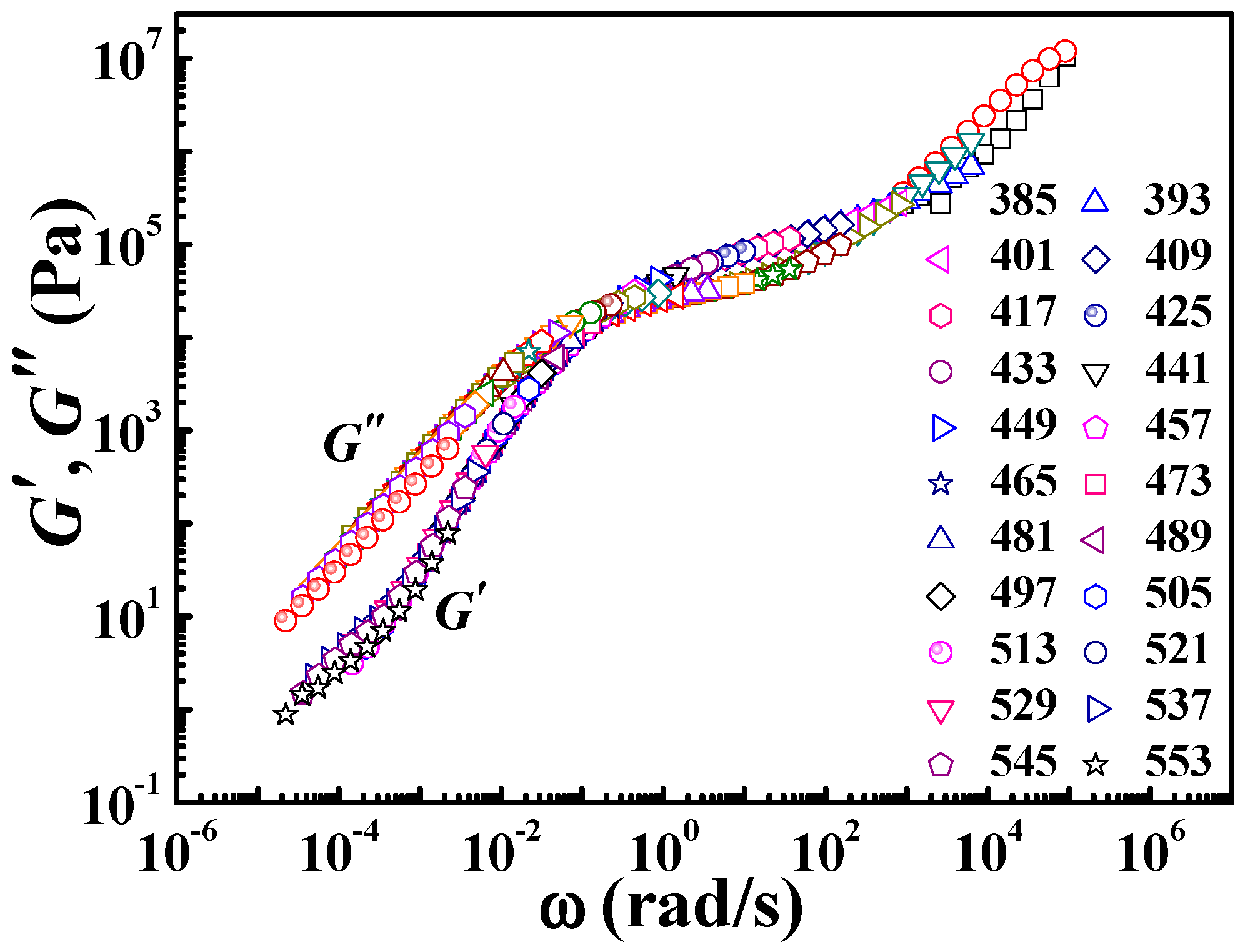
Ts = 425 K was chosen as the reference temperature, about 50 K higher than its
Tg (378 K). The master curve at the reference temperature can be obtained by horizontal shifting of frequency (
ω) dependence (from 0.1 rad/s to 10 rad/s) of
G′ and
G″ at different temperatures from 385 K to 553 K, as shown in
Figure 8. The temperature range here covers both regions, i.e., the vicinity of glass transition and high temperatures far away from
Tg + 100 K.
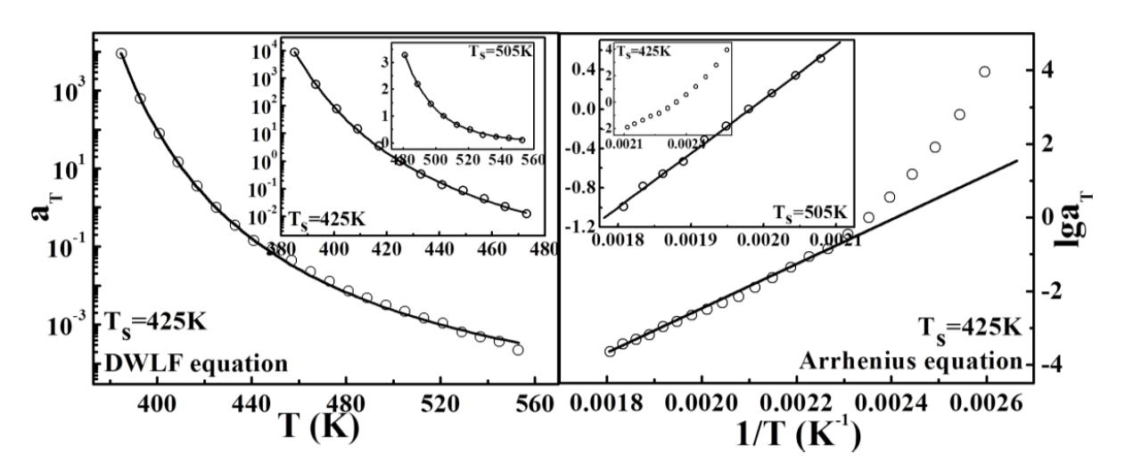
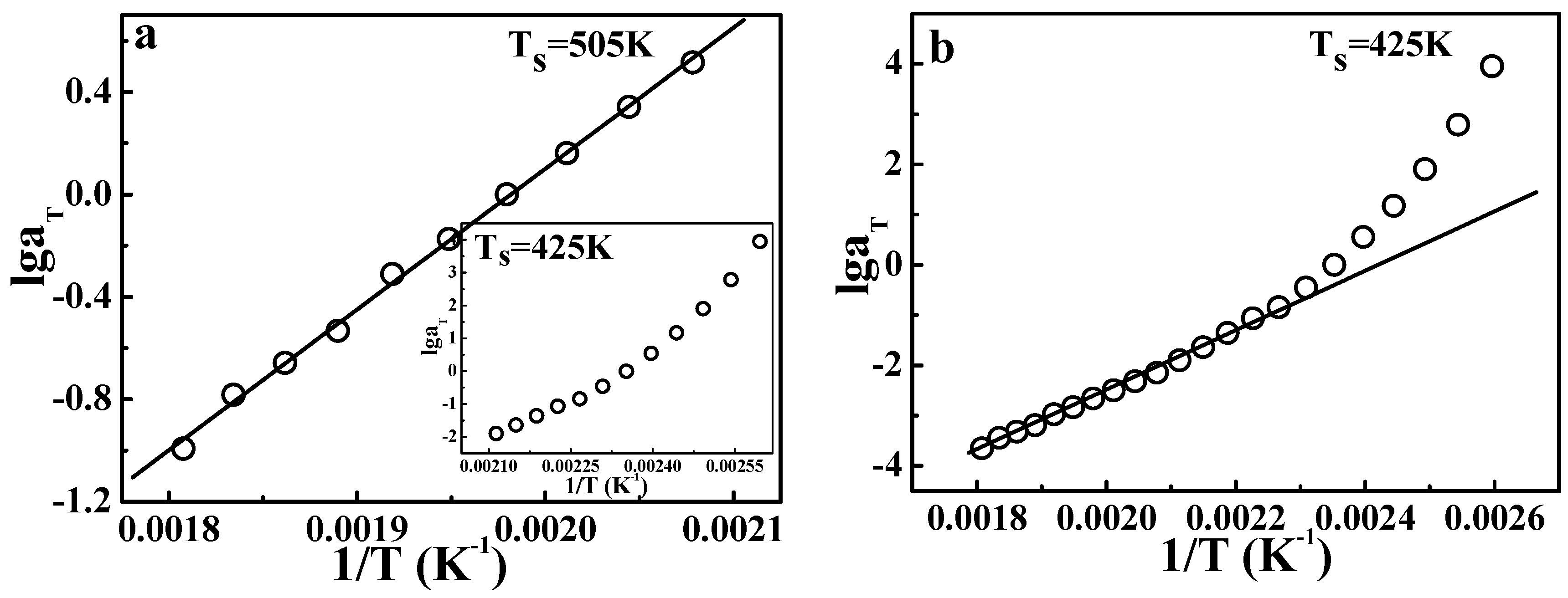
Figure 9 gives the results of TTS described by the Arrhenius equation.
Figure 9a shows the application of the Arrhenius form at temperatures from 481 to 553 K, and the insert gives the result from 385 to 473 K. Legitimately, the points at high temperatures (481 to 553 K) show a good linear relationship, according to the Arrhenius equation. However, the insert in
Figure 9a shows a curve, not a line, indicating that in the vicinity of glass transition, the Arrhenius equation is no longer valid. These results are consistent with our common knowledge. Of course, the Arrhenius equation is invalid in the whole temperature range also, as shown in
Figure 9b. This fact also means that at temperatures from 385 to 473 K, the apparent activation energy shows a strong dependence on the temperature.
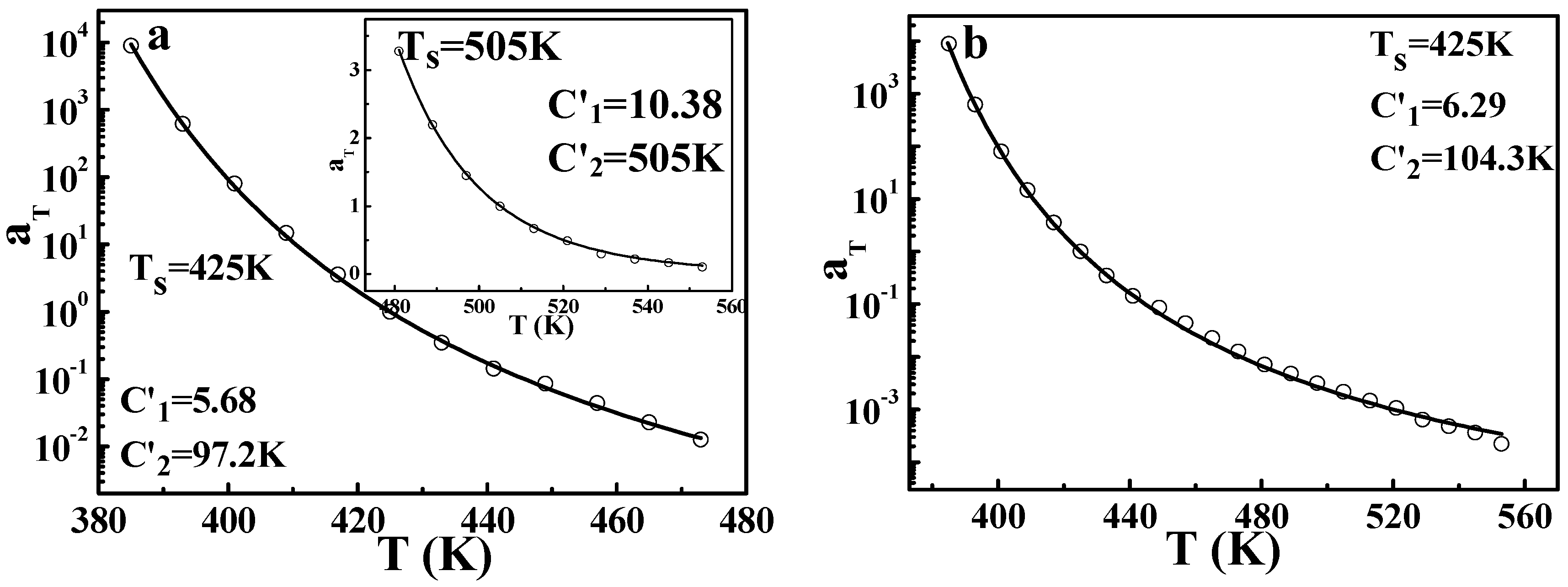
Based on the results and discussions above, the DWLF equation can be applicable at very high temperatures. In addition, the vicinity of glass transition is also the traditional region in which the WLF form is valid. Consequently, it is interesting whether the DWLF equation can be availably applied to the whole temperature range. Differing from that of the Arrhenius form, it is found that the DWLF equation can be applied in both regions well, as shown in
Figure 10a. In the vicinity of glass transition (from 385 to 473 K), the two parameters are
C1′ = 5.68 and
C2′ = 97.2 K, differing from the empirical values (
C1 = 8.86 and
C2 = 101.6 K) when the reference temperature is located roughly 50 K above
Tg [
2]. Additionally, at high temperatures, the DWLF equation also accords with the data perfectly, shown as the insert in
Figure 10a, provided
Ts =
C2′ according to the criterion above. Moreover, in the whole temperature range, the TTS of the viscoelastic behavior for PS can be described by the DWLF equation excellently again, indicating that Equation (9) is indeed universal for a wide temperature range. In view of the larger value of
C2′ in
Figure 10b (
C2′ = 104.3 K) than that in
Figure 10a (
C2′ = 97.2 K), this means that due to the higher temperature, the DWLF equation approaches the Arrhenius form more and more. When the temperature region is wholly higher than
Tg + 100 K, the value of
C2′ is equal to
Ts, shown as the insert in
Figure 10a.
In addition, the TTS of other pure polymers, for example, PMMA, is also investigated.
Figure 11a shows the master curve of PMMA at
Ts = 423 K (for PMMA,
Tg = 370 K, as seen in the
Supporting Information). Similar to PS, the master curve of PMMA at the reference temperature can be obtained by horizontal shifting of the frequency (
ω) dependence of
G′ and
G″ at different temperatures. The application of the DWLF equation is displayed in
Figure 11b. All the data points show the consistency with the DWLF curve, meaning the DWLF equation is also valid within the wide temperature range from
Tg to very high temperatures in this case.
The results above have indicated that the DWLF equation is universal at temperatures above
Tg. When the temperature is much higher than
Tg + 100 K, the DWLF equation evolves into the Arrhenius form. Based on this concept the Arrhenius form may be expressed as:
In the vicinity of glass transition, the item T2/(C2′ + T − Ts)2 depends on temperature strongly, meaning a strong temperature dependence of apparent activation energy. When the temperature is far away from the glass transition, C2′ approaching Ts will result in being one for this item, meaning that the apparent activation energy becomes approximately temperature-independent.
As pointed out in the Introduction, the Arrhenius form can describe both the terminal relaxation and secondary relaxation of polymers. In the discussion above, it has been proven that the DWLF equation can be universal at temperatures above
Tg. However, a question arises: is it appropriate to use the DWLF equation on the secondary relaxation of polymers? Based on the equivalence of the DWLF equation to the Arrhenius form at
C2′ =
Ts, it seems no obstruction for the application on secondary relaxation.
Figure 12 gives the results of the secondary relaxation of PMMA, which has been described by the Arrhenius form in our other paper [
18]. It is seen that the DWLF equation can also describe the secondary relaxation well. The apparent activation energy of secondary relaxation obtained by the DWLF equation is ♦
Ea = 80.5 ± 0.2 kJ/mol, which is near that obtained by the Arrhenius form (♦
Ea = 84.1 ± 0.2 kJ/mol) [
18]. Thus,
Figure 11 and
Figure 12 indicate the fact that the DWLF equation can describe the relaxation behavior of the polymer from secondary relaxations to the terminal flow according to two different reference temperatures: one is for secondary relaxation and the other for those above
Tg.
To examine the effectiveness of the DWLF equation in describing secondary relaxations further, the
β-relaxation process of PVC was also studied.
Figure S8 (seen in the
Supporting Information) shows that the
β-relaxation of PVC occurs at about 253 K at 1 Hz. When the frequency decreases, the temperature at which
β-relaxation occurs also decreases. Therefore,
αT obtained from different frequencies can be described by the DWLF equation and the Arrhenius form. The results are given in
Figure 13. Both equations can describe the
β-relaxation behavior well. Moreover, the apparent activation energies obtained from the two equations are also approximate, i.e., ♦
Ea = 205 ± 6.9 kJ/mol for the DWLF equation and ♦
Ea = 181.8 ± 7.2 kJ/mol for the Arrhenius form, respectively.
3.5. Theoretical Analysis of the Universal Application of the DWLF Equation
The results and discussions above have shown that the Arrhenius form is the limiting form of the WLF (VFTH) equation provided T∞ = 0, and the DWLF equation can be applicable in a wide temperature range if there are rational values of C1′ and C2′. However, the rationality of T∞ = 0 is based on ignoring the physical meaning of T∞. In this section, the operation of T∞ = 0 will be discussed theoretically.
According to the thermodynamic theory of glass transition by Gibbs and DiMarzio [
33,
34,
35,
36], glass transition is indeed a true second-order transition, and the true equilibrium
Tg (defined as
T2) can be obtained only at infinitely long times, which is difficult to realize. In infinitely slow experiments, no discontinuity will be observed in the first-order properties (volume and internal energy) at
T2, but the second-order properties (thermal expansion coefficient and heat capacity) will exhibit discontinuous change [
37]. The equilibrium
Tg (
T2) at which the conformational entropy of the polymer is zero always lies about 50 K below the
Tg observed at ordinary times for most polymers [
7,
38]. On the other hand, Fox and Flory first used the free volume theory to explain the glass transition of polymers [
37,
39]. The core idea of free volume theory can be described by
Figure 14 in which
ν(T) is total specific volume,
ν0,
νf is occupied volume and free volume, respectively, and
νg is specific volume at
Tg [
1,
27]. In this theory, the glass state is an iso-free-volume state for all polymers. In the glass state, thermal expansion is only contributed to by the expansion of occupied volume; while in the rubber state, thermal expansion is contributed to by both occupied volume and free volume. Since segment motion depends on the free volume, at temperatures below
Tg, chain segments are frozen and cannot move due to the freezing of the fractional free volume. According to free volume theory,
Tg can be determined as the temperature at which the thermal expansion coefficient undergoes a discontinuity during cooling. Considering the fact that the conformational entropy of the polymer is zero at equilibrium
Tg, according to the Gibbs–DiMarzio theory [
7,
33,
34,
35,
36,
38], the equilibrium
Tg must be the temperature at which the fractional free volume is zero since the conformational entropy can be zero only in the case that there is not any free volume according to the free volume theory [
1,
37,
39]. Moreover, Sperling [
7] pointed out that free volume shrinks very slowly with decreasing temperature even in the glass state. If temperature decreases with an infinitely slow rate, the equilibrium fractional free volume can be obtained during the whole experiment, shown as the short dashes in
Figure 14 [
27]. This equilibrium line of
ν(
T)/
νg will intersect with the line of
ν0(T)/
νg. It is easy to understand that the fractional free volume at the crossover point is zero from
Figure 14. Consequently, the conformational entropy of the polymer at this state is zero since there is not any free volume to realize the movement of chain segments. That means that
T∞ in
Figure 14 is the equilibrium
Tg. From
Figure 14, it is easy to obtain:
Considering the fact that fractional free volume in the glass state is 0.025 for most polymers and
αf = 4.8 × 10
−4 K
−1 [
1,
2], we have [
27]:
That value is consistent with the Gibbs–DiMarzio theory in which equilibrium
Tg always lies about 50 K below the apparent
Tg [
7,
38]. In view of the discussions on the VFTH equation in
Section 3.1, it is easy to understand that the so-called Vogel temperature
T∞ in the VFTH equation is also just the equilibrium
Tg in
Figure 14 according to the Adam–Gibbs theory [
3]. When
Tg is chosen as
Ts in the WLF form, it can be concluded that there are universal values of
C1 and
C2 for most polymers according to Equations (3), (4) and (19).
Since the mobility of chain segments depends on the free volume, the temperature dependence of the relaxation for polymers indeed depends on free volume [
1]. The free volume dependence of relaxation is successfully applied by Doolittle in his viscosity equation [
24,
40,
41,
42,
43]:
where
A and
B are empirical constants. On the other hand, the diffusion coefficient (
D) of entangled linear polymers in the molten state can be obtained according to de Gennes [
44,
45],
in which
k is the Boltzmann constant,
T is absolute temperature,
is the friction coefficient,
Ne is the number of Kuhn monomers in an entanglement strand and
N is the number of Kuhn monomers in a macromolecular chain. Equation (21) indicates that the relaxation of polymers is also influenced by the specific chemical structure. Consequently, it is reasonable to say that the potential energy barrier (
Ea) for relaxation should be composed of two items, i.e.,
in which
Ef stands for the contribution of free volume and
Es stands for the contribution of the specific chemical structure. According to the pioneering work of Turnbull and Cohen on free volume theory [
46,
47], it is pointed out that at small
νf, considerable energy is required to redistribute the free volume; while when
νf is larger than a critical value, the free volume can be redistributed freely. When the temperature is near the glass transition, the molecular relaxation rate is strongly limited by the large energy barrier, which is required for redistributing the free volume [
47,
48]. Therefore, it can be obtained:
From
Figure 14, it is easy to obtain:
in which
A is the value of
ν0/
νg at 0 K and
K1 and
K2 are constants.
As for
Es, it must be related to the difficulty of internal rotation since different conformations of the polymer can be converted to each other through internal rotation of a single bond. Therefore, the interaction between monomers induced by the chemical structure certainly influences the motion of chain segments. Consequently, it can be obtained:
where
ε stands for the structural barrier of internal rotation. Therefore, we have:
The first two items are determined by the free volume, and the last item is determined by the chemical structure. Near the glass transition,
T is approximate to
T∞. In this case, (
K1/(
T −
T∞) +
K2/(1 −
T∞/
T))
ε, indicating that
Ea strongly depends on
ν0/
νf. That is the reason why Equation (20) can be used only in the glass transition region [
46]. At high temperatures far the above glass transition,
T T∞, meaning
K1/(
T −
T∞) is very small and
K2/(1 −
T∞/
T) is approximate to
K2. In this case,
Ea strongly depends on
K2 +
ε, indicating that
Ea shows weak temperature dependence at high temperatures. This fact is consistent with the Arrhenius form (Equation (5)) in which the apparent activation energy is independent of temperature.
Figure S9 (seen in the
Supporting Information) shows the activation energies of PS and PMMA. It can be seen that the activation energy at low temperatures near the glass transition shows a strong temperature dependence, and at high temperatures, it shows a weak temperature dependence. This fact is consistent with the discussions above. On the other hand, as for the VFTH form (Equation (2)), it can be expressed as:
In view of the form of Equation (27) and item
K1/(
T −
T∞) +
K2/(1 −
T∞/
T), it is easy to understand that the apparent activation energy of the VFTH form only depends on
K2/(1 −
T∞/
T). Obviously, that means that the value of
ν0/
νg at 0 K is too small, leading to the rationality of ignoring the item
K1/(
T −
T∞). In addition, it can be seen that the value of
T∞ can regulate the temperature dependence of
Ea according to Equation (26). When the value of
T∞ is large,
Ea shows a strong temperature dependence; while
T∞ is small,
Ea shows a weak temperature dependence. In the case of
T∞ = 0,
Ea ≈
K2 +
ε, showing the independence of temperature. In that case, Equation (27) possesses constant activation energy, equal to the Arrhenius form. Therefore, it can be revealed that the operation of
T∞ = 0 in
Section 3.1 is to regulate the temperature dependence of
Ea; in fact, resulting in the equivalence of the VFTH form to the Arrhenius form.
In addition, if the DWLF equation can be applicable in a wide temperature range from
Tg to very high temperatures, its activation energy should show a similar temperature dependence of (
K2/(1 −
T∞/
T) +
ε) according to Equation (26) (item
K1/(
T −
T∞) is ignored). Since Equation (11) can be expressed as:
and
R,
C1′,
C2′ and
Ts are all constants, the temperature dependence of ∆
just depends on the item
X1/(1 −
X2/
T)
2.
X1 and
X2 are adjustable parameters. This form is similar to
K2/(1 −
T∞/
T), meaning that
∆ can be approximate to
K2/(1 −
T∞/
T) +
ε and show a similar temperature dependence when appropriate values for
R,
C1′,
C2′ and
Ts are adopted. As a result, the DWLF equation can be applied in wide temperature range.
In addition, if Equation (4) is introduced into Inequality (14), we have:
That means that although the DWLF equation can be used over a wide temperature range, it should be used only above the equilibrium glass transition. This result is consistent with Equation (26). When
T is below
T∞, the first two items in Equation (26) representing the contribution of free volume are both negative values, which are meaningless. This fact indicates in the case of the application in a continuous wide temperature range, the DWLF equation can and must be applicable above the equilibrium glass transition to high temperatures. As for describing the secondary relaxations, the DWLF equation should be used only in the case of
T∞ = 0, i.e.,
C2′ =
Ts. In that case,
Ea ≈
K2 +
ε (according to Equation (26)), independent of temperature, and thus, the DWLF (or VFTH) equation is equivalent to the Arrhenius form. However, it should be pointed out that when
T∞ = 0, although the DWLF equation is equivalent to the Arrhenius form and thus can describe the secondary relaxations just as shown in
Figure 12 and
Figure 13, this equation cannot be applicable at a wide temperature range since
Ea ≈
K2 +
ε shows no temperature dependence.
Based on the above results and discussions, we propose a developed WLF equation that can be universal for polymers from glass transition to terminal relaxation and also applicable for secondary relaxations. Furthermore, we explain why the DWLF equation can achieve the time-temperature superposition of the relaxation properties of polymers in a wide temperature range theoretically. The Arrhenius form is the limit form of the DWLF equation or the VFTH equation. Based on this viewpoint, it is reasonable to draw the conclusion that there should be a universal essential mechanism for different relaxations of polymers.


