Can a Combination of UAV-Derived Vegetation Indices with Biophysical Variables Improve Yield Variability Assessment in Smallholder Farms?

Abstract

The rapid assessment of maize yields in a smallholder farming system is important for understanding its spatial and temporal variability and for timely agronomic decision-support. We assessed the predictability of maize grain yield using unmanned aerial/air vehicle (UAV)-derived vegetation indices (VI) with (out) biophysical variables on smallholder farms. High-resolution imageries were acquired with UAV-borne multispectral sensor at four and eight weeks after sowing (WAS) on 31 farmer managed fields (FMFs) and 12 nearby nutrient omission trials (NOTs) sown with two genotypes (hybrid and open-pollinated maize) across five locations within the core maize region of Nigeria. Acquired multispectral imageries were post-processed into three VIs, normalized difference VI (NDVI), normalized difference red-edge (NDRE), and green-normalized difference VI (GNDVI) while plant height (Ht) and percent canopy cover (CC) were measured within georeferenced plot locations. Result shows that the nutrient status had a significant effect on the grain yield (and variability) in NOTs, with a maximum grain yield of 9.3 t/ha, compared to 5.4 t/ha in FMFs. Generally, there was no relationship between UAV-derived VIs and grain yield at 4WAS (r < 0.02, p > 0.1), but significant correlations were observed at 8WAS (r ≤ 0.3; p < 0.001). Ht was positively correlated with grain yield at 4WAS (r = 0.5, R² = 0.25, p < 0.001) and more strongly at 8WAS (r = 0.7, R² = 0.55, p < 0.001), while the relationship between CC and yield was only significant at 8WAS. By accounting for within- and between-field variations in NOTs and FMFs (separately), predictability of grain yield from UAV-derived VIs was generally low (R² ≤ 0.24); however, the inclusion of ground-measured biophysical variable (mainly Ht) improved the explained yield variability (R² ≥ 0.62, Root Mean Square Error of Prediction, RMSEP ≤ 0.35) in NOTs but not in FMFs. We conclude that yield prediction with UAV-acquired imageries (before harvest) is more reliable under controlled experimental conditions (NOTs), compared to actual farmer managed fields where various confounding agronomic factors can amplify noise-signal ratio.

1. Introduction

Rapid assessment of crop yield is critical in order to monitor and address yield gaps [1,2], yet robust sampling is often cost-intensive across agricultural fields or landscapes. Hence, technologies and methods that can provide leverage for quick and non-destructive data collection are critical for monitoring changes both spatially and temporally. The evolution of remote-sensing technologies for the acquisition and processing of remotely-sensed imageries is considered valuable for the assessment of yield or other agronomic variables at various scales [2,3]. However, access to high-quality imageries is generally constrained by associated costs and time-lag in processing, posing limitations to the prospects of utilizing imagery-derived data for various agronomic use-cases, both in-season and out-of-season. Yet, there is a critical need to evolve reliable and rapid approaches for timely decision support within smallholder farming systems. Smallholder farming systems of sub-Saharan Africa (SSA) are often characterized by fragmented farmlands and differentiated management practices [3,4,5,6]. Most landscapes are complex mosaics with diffuse field boundaries and trees. Therefore, imageries of the landscape need to have sufficient spatial and temporal resolution to mask out areas of vegetation or undesired features. Spatially-explicit data acquired over farming landscapes can improve the understanding of the variability and dynamics of agronomic processes and variables, especially in smallholder cropping systems where changes may be more frequent at smaller scales, including within farm fields. Quite often, these changes are influenced by the management preferences of the farmers whose decisions are mostly driven by various external factors, including accessibility and affordability of inputs [7,8]. Most smallholder farming landscapes are defined by different varieties that are sown on different dates, with different soil nutrient application or status. Consequently, they are often characterized as mosaic(s) of individual fields that have contrasting vegetation structures or types within a very small area (often, within tens of meters).

The recent advances in satellite-based remote-sensing of global land-cover coincides with the emergence of unmanned aerial/air vehicles (UAVs) for crop monitoring and yield assessment, with increasing application for agronomic decision-support across large-scale mono-cropped and smallholder multi-cropped farming systems [9,10,11]. UAVs were initially developed for military use but have become recognized as a tool to acquire high-resolution imageries that can be post-processed and analyzed to understand spatially varying agronomic factors at the field scale. Within the past five years, several researchers have reported the applicability of UAV for monitoring agronomic variables, e.g., [11,12,13], in different cropping systems and across diverse geographies [10,14,15,16]. Many of these variables are considered as potential proxies for yield estimation [10,14,15], especially at the plot and field level (typically up to 1000 ha). There are several existing methods for estimating crop yields with remote-sensing. A popular approach is to relate measured location-specific yields to vegetation indices (VI) derived from RGB, multi-spectral, or hyper spectral camera sensors. VIs often provide strong expression of the ground cover and the chlorophyll content of green material [17,18]. Many VIs have been developed, with the most common being the normalized difference vegetation index (NDVI) [10,11,19,20,21]. Based on varied relationships between different reflectance spectral bands, other VIs have also evolved with a strong relevance for agricultural systems. These include the normalized difference red-edge (NDRE), green normalized difference vegetation index (GNDVI), green canopy vegetation index (GCVI), red vegetation index (RVI), red-edge canopy index (RECI), and many others [22,23]. Because these VIs represent spectral (and to a lesser extent, structural) characteristics of the vegetation, they are potential proxies for rapid assessment of yield and yield variability. Further, when these VIs are derived from spatially-explicit remotely-sensed imageries, they can provide a very useful understanding of yield variability at varying spatial scales. For instance, the use of individual VIs for the diagnosis of nutrient constraints and crop yield differences between fields/plots have been promising, e.g., [12,14]. Further, researchers have proposed that a combination of VIs can provide additive sensitivity effect and improve the detectability of nuanced vegetational characteristics to improve the assessment of agronomic parameters, including yield, e.g., [23,24]. This is because single VIs can be constrained by vegetation structure and composition, which may be undetectable at specific wavelengths of the electromagnetic spectrum. Researchers [21,25,26] have suggested that the greenness of plants grown under adequate nutrient conditions can compromise the accuracy of the remotely-sensed NDVI (from the multispectral sensor) due to saturation within the green spectral band. This type of limitation can be avoided by using other VIs that rely on spectral information from other reflectance bands within the electromagnetic spectrum.

While the use of UAVs for agronomic decision-support is fast evolving [11], there are limitations. For instance, Watanabe et al. [27] indicated that sorghum plant height was overestimated by UAV and that high fertilization affected the relationship between UAV and ground-based measurements. Schut et al. [28] reported that vegetation indices did not capture all management and biophysical factors that can aid the accurate assessment of yield within fields. Yet, new generation UAV-borne sensors may offer improved assessment accuracies for crop monitoring, especially in combination with (few) ground level data [29,30]. According to Sibley et al. [31] and Schut et al. [28], repeated in-season measurements and good field-level accuracy are important criteria that can be used to derive useful information from remotely-sensed imageries for rapid yield (and other agronomic) assessments. Given the complexity of smallholder farming systems [2,6], it is important to assess the field applicability of UAV beyond experimental plot conditions and within complex farming landscapes, where they can be used for rapid farm-level decision support. Schut et al. [28] indicated yield variability explained by selected VIs within specific crop farms reduced greatly across an array of fields compared to within fields where there is a higher homogeneity, and they noted that accurate ground reference data may improve the assessment of in-season yield variability. These ground data can include biophysical variables, such as plant height (Ht) and canopy cover (CC), which have been reported as valuable for non-destructive yield(-variability) assessment in smallholder farmers’ fields. These biophysical variables represent morphological characteristics and are useful for understanding the allometric characteristics of plants [2]. Therefore, this study was conducted within the maize-producing savanna region of Nigeria to assess in-season predictability of grain yield in multilocational smallholder maize farmers’ fields using UAV-derived VI with and without ancillary observations of biophysical variables. Our objective is to advance knowledge on the application of UAVs for in-season monitoring of maize yield in farmers’ fields by combining ground-measured biophysical variables with UAV-derived VIs to assess yield variability.

2. Materials and Methods

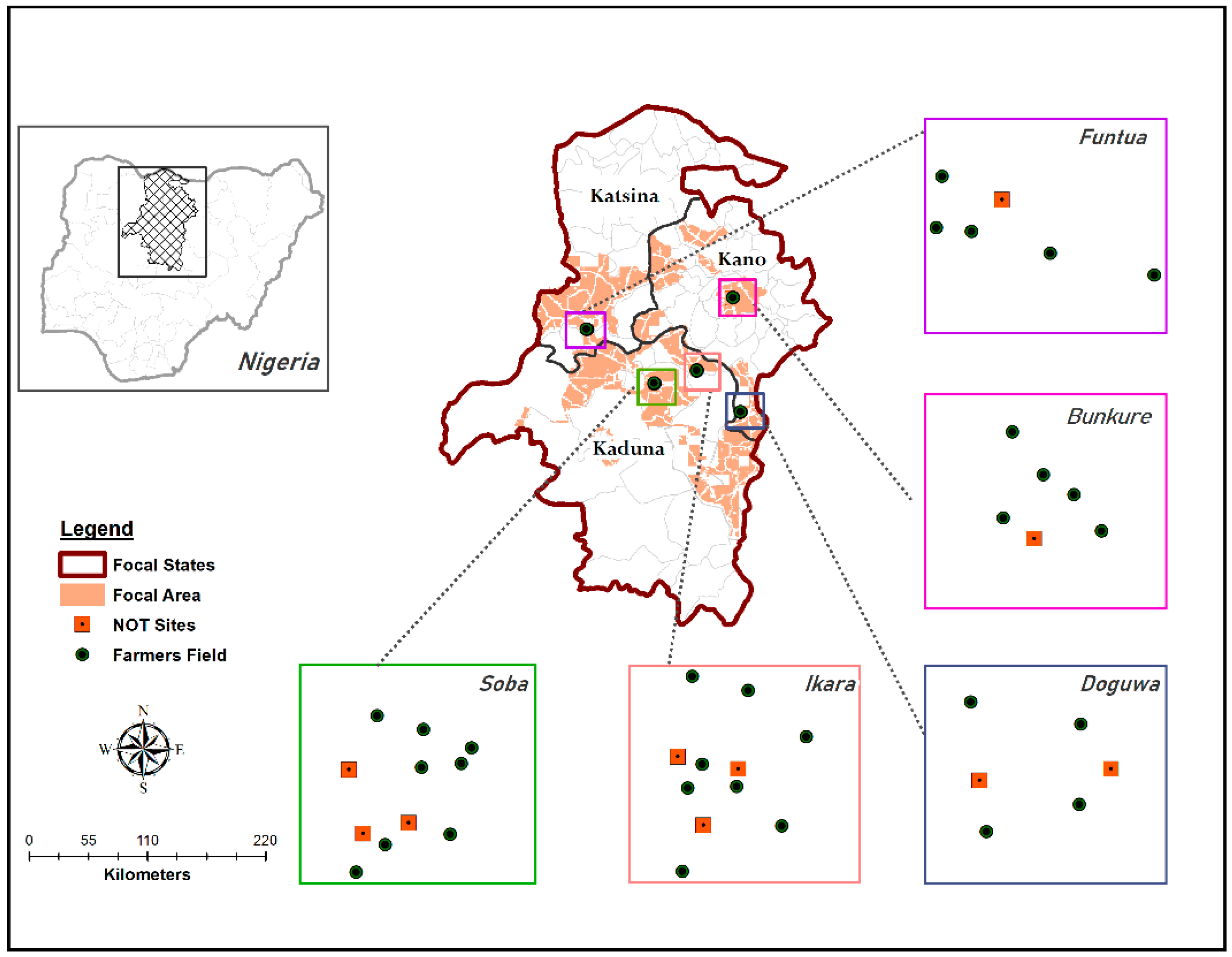
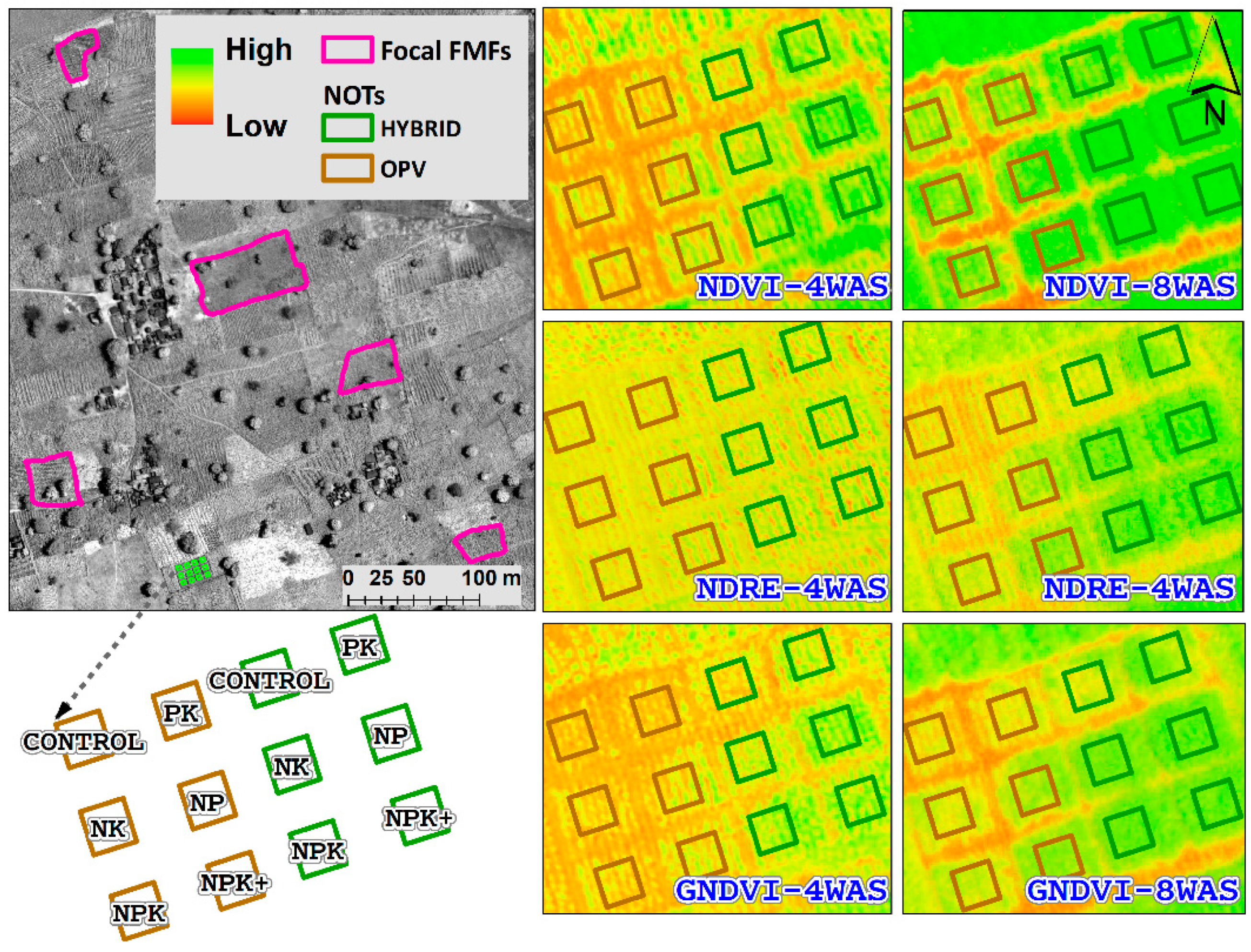
2.1. Study Area

This study was carried out at multiple locations within the core maize production region of Nigeria; namely, Bunkure, Doguwa, Funtua, Ikara, and Soba (Figure 1). The locations are within the Sudan and Northern Guinea savanna agroecological zones of the Country, which is the major cropping regions for grains and legumes such as maize (Zea mays L.), cowpea (Vigna unguiculata L.), peanut (Arachis hypogaea L.), and soybeans (Glycine max L.). The target areas for UAV-based data collection were selected based on: (i) the location of nutrient omission trials (NOTs), which were established under a different research activity to identify and understand nutrient constraints that are limiting maize yield among smallholder maize farmers [32]; (ii) the willingness of proximal farmers to grant access for ground-truthing and yield assessment in their farms, and (iii) the advisory guidance of the National Space Research and Development Agency (NASRDA) in Nigeria, which is critical for compliance with regulatory requirements on UAV use in the Country. The study area is characterized by a growing period of 151–160 days, mean annual rainfall of 800–1250 mm, and daily mean minimum and maximum temperature of 12 °C and 32 °C, respectively. Rainfall is unimodal and lasts from June to October, is considerably optimal for grain crops, and is well distributed throughout the growing season, while the dry season starts from late October to May.

2.2. Smallholder Farmers’ Fields and Nutrient Omission Trials (NOTs)

2.2.1. Nutrient Omission Trial Field Establishment

At the onset of the planting season for the region, from mid to late June 2016, NOTs (n = 100) were established to assess the impact of varying soil nutrient limitations on maize yield within the maize-based system of Nigeria under the Taking Maize Agronomy to Scale in Africa (TAMASA) project (www.tamasa.cimmyt.org; [32]). A subset of the NOTs (n = 12) were covered within the target locations for UAV flight. Each experimental unit was comprised of 12 contiguous plots (5.2 m × 4 m) planted with maize in two blocks of six plots, with one block sown with open-pollinated genotype (OPV) and the other sown with hybrid genotype (HV). Within each of the genotype blocks, the nutrient treatments comprised a combination of major nutrients required for maize production, including nitrogen (N), phosphorus (P), potassium (K), and micronutrients (+). Hence, each genotype block received six fertilizer treatments (i.e., Control, PK, NP, NK, NPK, and NPK+) applied on six plots across twelve (12) multilocational NOTs, which were applied at recommended optimal dosage [32] based on previous soil tests in the region. Therefore, a total of 144 plots were covered during flight missions at 4 and 8 weeks after sowing (WAS) across the entire study location. All nutrients were applied at the establishment stage of NOT, except for N, which was applied in 3 splits (at establishment, 3WAS, and 6WAS). Other details on rates and management of NOTs are presented by Shehu et al. [32].

2.2.2. Farmers’ Fields

Because farmers made their farm-level decisions independent of our research interests, we screened prospective volunteer farmers to select only farmlands that were sown with maize within about 3 days of NOT establishment. The selected farmers’ fields (n = 32) differed in size and management; this is typical within smallholder maize-based systems. The specific genotype choice of the farmers is generally unknown; however, within the maize-based area, farmers sow both the open-pollinated (OPV) and hybrid (HV) genotypes.

2.3. UAV-Based Acquisition of Imageries and Post-Processing

We used an eBee UAV (SenseFly Inc., Switzerland, www.sensefly.com/drone/ebee.html) mounted with multispectral 4C sensor (Airinov, France, www.airinov.fr) to acquire fine resolution imageries at each target location. The e-Bee is a light-weight fixed-wing UAV that can cover up to 600 ha in a single flight at 1000 m altitude and is equipped with an onboard global positioning system (GPS), solar irradiance sensor, and a ground calibration target. The multi-spec 4C camera has four passive sensors that record reflectance in four spectral bands: red (R), green (G), red-edge (RE), and near infra-red (NIR) at 1.2 megapixels per sensor. It has a global shutter, instant field of view (IFOV) of 0.9 mrad, and low luminosity (>3000 lux). The UAV was flown to acquire fine-resolution imageries that covered the area of interest (including NOT and farmers’ fields) at 4 and 8WAS, coinciding with the onset of vegetative (V7) and tasseling (VT) growth stages, respectively [33], and within the mid-season growth period where best indication of post-harvest grain yield is obtainable [34].

Post-Processing

After the completion of each flight mission, the imageries were exported from the UAV along with the flight log files for post-processing with Pix4D software (Pix4D v.3.1., Switzerland, www.pix4d.com). The software provided a platform for end-to-end post-processing of the acquired imageries and offered the needed flexibility to configure processing parameters based on desired output quality and target end-use of the products. Overall, for each successful flight mission, ~400 imageries were geotagged and processed through several stages to generate final outputs in geotiff formats, including reflectance bands corresponding to the four spectral reflectance domains of the multi-spec sensor, digital surface model, digital orthomosaics, and VIs. The VI imageries were computed from corresponding spectral bands, based on Equations (1)–(3). The consideration of VIs to be computed was limited to those that had been reported as promising for agronomic application at the canopy level and in relation to vegetation status in croplands, especially maize, with a focus on selecting VIs that were based on red, red-edge, and green bands [23,35,36,37,38].

$$\mathrm{NDVI}=\frac{\mathsf{\rho }\mathrm{nir}-\mathsf{\rho }\mathrm{red}}{\mathsf{\rho }\mathrm{nir}+\mathsf{\rho }\mathrm{red}}$$

(1)

$$\mathrm{NDRE}=\frac{\mathsf{\rho }\mathrm{nir}-\mathsf{\rho }\mathrm{red}.\mathrm{edge}}{\mathsf{\rho }\mathrm{nir}+\mathsf{\rho }\mathrm{red}.\mathrm{edge}}$$

(2)

$$\mathrm{GNDVI}=\frac{\mathsf{\rho }\mathrm{nir}-\mathsf{\rho }\mathrm{green}}{\mathsf{\rho }\mathrm{nir}+\mathsf{\rho }\mathrm{green}}$$

(3)

where $\mathsf{\rho }\mathrm{nir},\mathsf{\rho }\mathrm{red},\mathsf{\rho }\mathrm{red}.\mathrm{edge},\mathrm{and}\mathsf{\rho }\mathrm{green}$ are the spectral reflectance of the near infrared band, red band, red edge band, and green band, respectively.

2.4. Ground-Truth Data Collection

We conducted in-situ measurement of NDVI with Greenseeker Handheld Crop Sensor HCS 100 (Trimble Ltd., Sunnyvale, CA; https://agriculture.trimble.com/precision-ag/products/greenseeker). The Greenseeker was held above the canopy (0.6 m) while walking for 30–60 s through each NOT plot, or through marked quadrats (4 m², n = 5) within each farmers’ field. The device proximally scans leaf greenness (within a swath of ~0.25 m) through its infrared sensors and displays an NDVI value averaged over the duration of the scan. We did not acquire ground-truth measurement for other VIs due to cost (money and labor) and because our goal was not to recalibrate the sensor, but rather to test the application of the UAV-borne multispectral sensor for assessing yield variability based on the indices derived.

We adopted the crop-cut method to quantify grain yield, as recommended by the FAO and generally regarded as the most objective method for yield estimation [14,39]. Harvest was conducted within 9 m² quadrats in each NOT treatment plot, based on standard NOT protocols, as presented by Nziguheba et al. [40]. In farmers’ fields, maize cobs were harvested and grain yield was quantified in five (2 m × 2 m) quadrats positioned along a diagonal transect within the field. In both farmers’ fields and NOTs, the harvested cobs were shelled, and the grain was oven dried to determine moisture content. The weight of grain yield per sampling quadrat were converted to yields in metric tons per hectare (t/ha) at 12% moisture content. The geographic coordinates were recorded as degrees latitude and longitude (position precision of ~3 m) at the center of each plot/quadrat in NOT and farmers’ field using a Garmin eTrex 20 GPS device (https://buy.garmin.com/en-US/US/p/87771#overview). Using a height ruler, we measured the height of three randomly selected maize stands within each quadrat, and the recorded values were later averaged per quadrat at 4WAS and 8WAS. Similarly, at both growth stages, we used the smartphone-based Canopeo app (http://canopeoapp.com/) to measure percent canopy cover in each quadrat, based on standard protocols [41].

2.5. Data Analyses

Data cleaning and multi-step spatial analyses of the data collected through ground measurements and UAV-derived datasets were conducted using ArcGIS 10.3.1 (ESRI, Redlands, California, http://www.esri.com/arcgis/about-arcgis) and open-source packages (including RGDAL, LMER, and GGPLOT) in R analytical platform v.3.4.1 (https://cran.r-project.org/bin/windows/base/old/3.4.1/).

2.5.1. Georeferenced Locations and Data Extraction

The recorded geographic coordinates (X, Y) were processed and exported into point shapefiles in WGS1984 datum in ArcMap. Using the UAV-derived imageries as reference, some misaligned coordinates were noted and corrected by editing the point shapefiles in ArcGIS. These misalignments were likely due to the precision level of the recreational GPS unit (~4 m); hence, the editing process was critical to ensure that each point shapefile location rested within the designated field and referenced the appropriate NOT plot or farmers’ field. Using the geoprocessing “Create Regular Polygon” add-on tool in ArcGIS, 4-sided polygons (2 m² for farmers’ field and 3 m² for NOTs) were generated for each ground-truthing point, using the point datasets as the centroid. These polygons represent the sampling support unit for the ground-truthing process and were subsequently used in R (Raster package [42]), to compute the zonal average statistics of UAV-derived VI cell values for each location at the matching support scale of the yield measurements.

2.5.2. Statistical Analyses of Data

Due to the slight skewness of the yield data, we applied log-linear transformation to normalize the dataset. The output from the spatial zonal statistics, which was computed from the UAV-derived imageries, was processed as a table and imported into R-Studio to assess the correlation of VIs with measured grain yield across the study locations, and separately within NOTs and farmer managed fields (FMFs). In the first level of the analyses, we used a linear multivariate regression approach (Equation (4)) to assess the variability of yield that is explained by ground-measured variables in NOTs.

$${\mathrm{yield}}_{\mathrm{i}}={\mathsf{\beta }}_0+{\mathsf{\beta }}_1{\mathrm{X}}_1+{\mathsf{\beta }}_2{\mathrm{X}}_2+{\mathsf{\beta }}_{\mathrm{i}}{\mathrm{X}}_{\mathrm{i}}+{\mathsf{\epsilon }}_{\mathrm{ij}}$$

(4)

where, ${\mathsf{\beta }}_0$ is the intercept and ${\mathsf{\beta }}_{1,2,\mathrm{i}}$ are slopes of the observed variables ${\mathrm{X}}_1$, ${\mathrm{X}}_2$, ${\mathrm{X}}_{\mathrm{i}}$, respectively.

In the second level, we independently and randomly split the NOT and FMF data into 70% calibration data (93 datapoints for NOT and 72 datapoints for FMF) and 30% validation data (37 datapoints for NOT and 27 datapoints for FMF). Some data records were excluded from further analyses in NOTs and FMFs due to irresolvable missing datapoints or incomplete records. The random split of each dataset was implemented at the Farm (i.e., field) level for independence of locations in the model calibration and validation stages. Notwithstanding the assumption that both NOT and FMF data belong to the same population (i.e., smallholder farmers), separate models were fitted for NOTs vs. FMFs. The calibration datasets were used to fit linear mixed effect models (Equation (5)) for yield prediction, using UAV-derived VIs at 4WAS and 8WAS as input variables, with and without the significant biophysical variables (as determined from the first step). The validation datasets were used to assess the accuracy of the prediction. Similar to Burke and Lobell [1], model fit was also applied to time series combination of 4WAS and 8WAS data to assess potential applicability for an improved prediction outcome (Equation (6)). The linear mixed effect modeling framework included a random parameter that accounts for the potential indeterminable effect of differing management practices among farmers. Statistical parameters that were evaluated to make inference include descriptive statistics (mean, range, coefficient of variation), correlation coefficient (r), coefficient of determination (R²), root means square error of prediction (RMSEP), and significance, P (tested at 95% confidence level). The best relationship between measured yield and UAV-derived VIs is indicated by r closer to 1, R² closer to 1, RMSEP closer to 0, and an acceptable significance level (p < = 0.05).

$${\mathrm{yield}}_{\mathrm{i}}={\mathsf{\beta }}_0+{\mathsf{\beta }}_1{\mathrm{VI}}_1\dots \dots \dots +{\mathsf{\beta }}_{\mathrm{i}}{\mathrm{X}}_{\mathrm{i}}+\left(1|\mathrm{Farm}\right)+{\mathsf{\epsilon }}_{\mathrm{ij}}$$

(5)

$${\mathrm{yield}}_{\mathrm{i}}={\mathsf{\beta }}_0+{\displaystyle \sum }_{\mathrm{t}=4}^{\mathrm{t}=8}{\mathsf{\beta }}_{1\mathrm{t}}{\mathrm{VI}}_{1\mathrm{t}}\dots \dots \dots +{\displaystyle \sum }_{\mathrm{t}=4}^{\mathrm{t}=8}{\mathsf{\beta }}_{\mathrm{it}}{\mathrm{X}}_{\mathrm{it}}+\left(1|\mathrm{Farm}\right)+{\mathsf{\epsilon }}_{\mathrm{ij}}$$

(6)

where, ${\mathsf{\beta }}_0$ is the intercept, ${\mathsf{\beta }}_1$ is slope of UAV-derived Vegetation Index, ${\mathrm{VI}}_1$, ${\mathsf{\beta }}_{\mathrm{i}}$ is the slope of measured biophysical variable ${\mathrm{X}}_{\mathrm{i}}$ (when included in the model), and t is the growth stage at which the imageries were acquired (in weeks after sowing (WAS)). The additional term, 1|Farm, denotes assignment of Farm as random variable where several factors can influence yield outcome.

3. Results

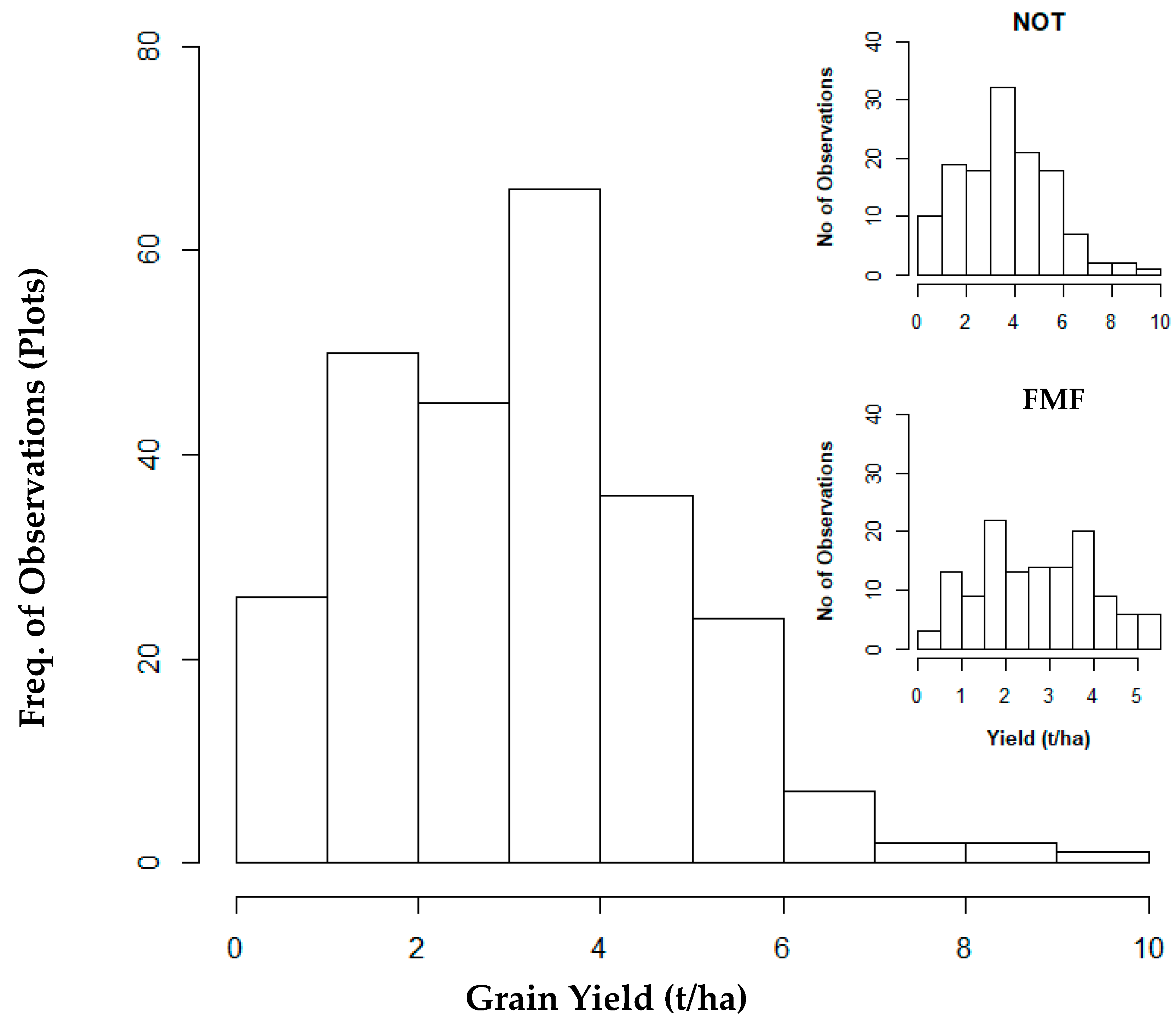
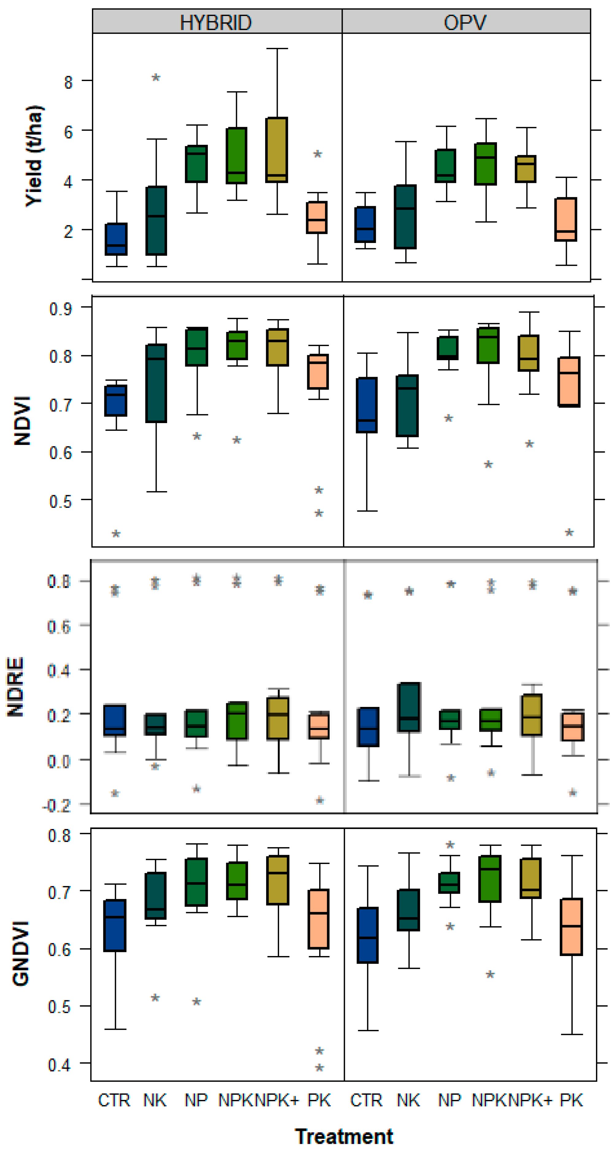
3.1. Estimated Grain Yield and Ground-Truth Biophysical Variables (gNDVI, Ht, and CC)

The overall average maize grain yield was 3.12 t/ha, with a lower average yield estimated in FMFs (2.75 t/ha) than the average yield across the NOT plots (3.6 t/ha;

Table 1. Summary of multivariate assessment of yield variability in nutrient omission trial (NOT) plots established at multiple locations within smallholder maize-based system of Nigeria.

Growth Stage	Source of Variation	DF	p-Value	Adj. R2
4WAS	Genotype	1	0.69	0.59 ***
	Treatment	5	<0.001
	Location	4	<0.001
	gNDVI	1	0.21
	Ht	1	<0.001
	CC	1	0.63
8WAS	Genotype	1	0.67	0.64 ***
	Treatment	5	<0.001
	Location	4	<0.001
	gNDVI	1	<0.001
	Ht	1	<0.001
	CC	1	0.04
4 + 8WAS	Genotype	1	0.66	0.67 ***
	Treatment	5	<0.001
	Location	4	<0.001
	gNDVI	1	<0.001
	Ht	1	<0.001
	CC	1	0.08

WAS denotes Weeks after Sowing, DF is the statistical degree of freedom, Adj. R² is the adjusted regression coefficient, gNDVI is the greenseeker measured normalized difference vegetation index, Ht is the Height, CC is the percent Canopy Cover, *** denotes high significance (p < 0.001) of the multivariate regression model.

). The maximum grain yield (9.3 t/ha) was attained by optimizing nutrient and genotype combination in NOTs, exceeding the maximum estimated yield in farmers’ fields (5.4 t/ha; Figure 2). In NOT plots, average ground-measured gNDVI, Ht, and CC increased from 4WAS to 8WAS across all treatments (Figure 3). Comparing treatments, the ground-measured variables were similar at 4WAS, but at 8WAS the NOT plots that received either NP, NPK, or NPK+ treatments showed significantly higher gNDVI, Ht, and CC (p > 0.001) compared to the Control, NK, and PK treatments.

The initial analyses of univariate relationships suggest that no correlation exists between grain yield and ground-measured variables (R² < 0.02; r < 0.14, Figure 4). However, by including the known explanatory variables (treatment, location, and genotype) into the linear multivariate model, the explained variation in yield greatly improved (R² = 0.45 for all data, R² = 0.67 for NOT, and R² = 0.14 for FMF). Additionally, the multivariate analysis of the NOT data showed that treatment and location, but not genotype, significantly explained the observed yield variability (R²= 0.50; p < 0.001). The average estimated yields for HV (3.41 t/ha) was comparable to OPV (3.68 t/ha), considering all locations and treatments.

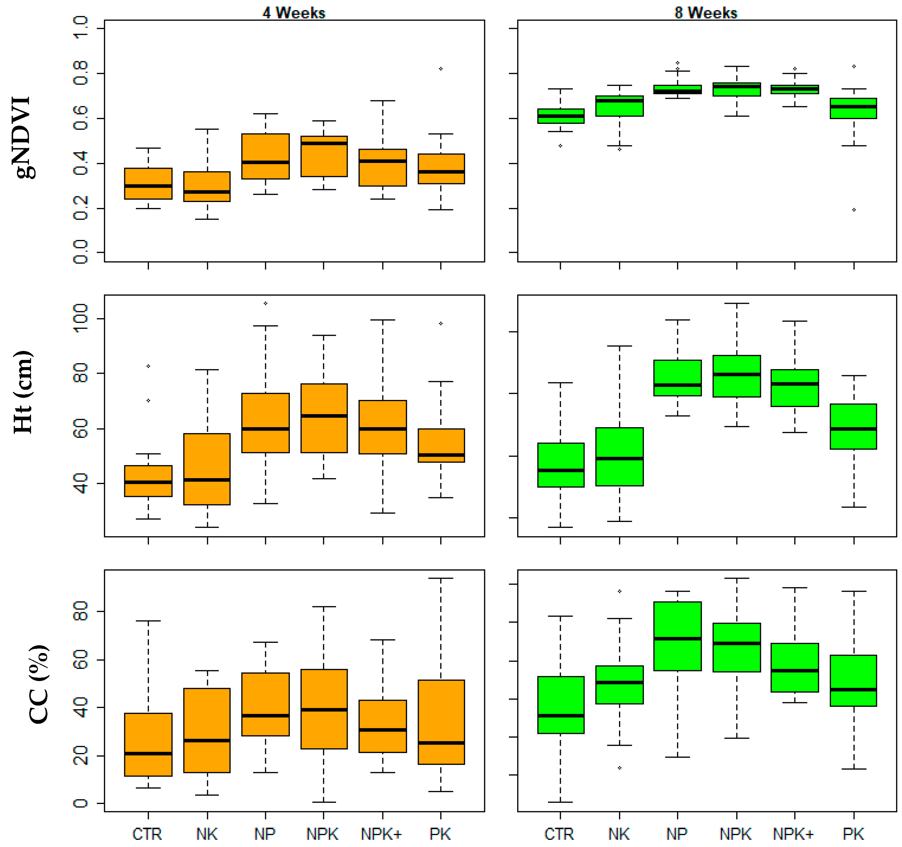
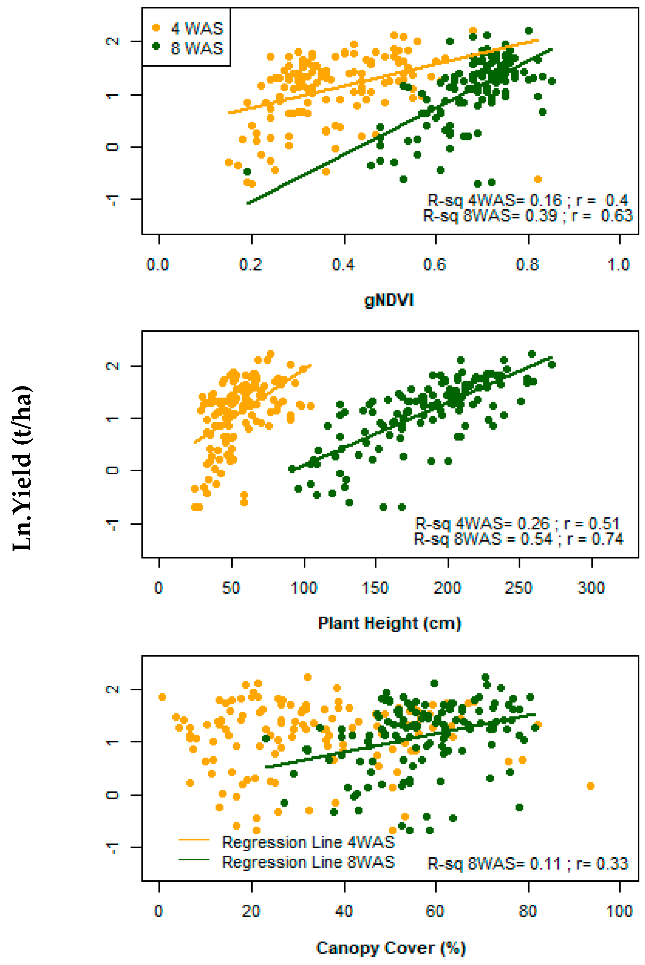
3.2. UAV-Derived VIs and Their Correlation with Yield in NOT and FMF

The imagery and extracted data from the UAV-derived VIs showed nutrient-induced differences in vegetational characteristics in the NOTs (e.g., Figure 5 and Figure 6) and general field-level variations across FMFs, with an observable transition between 4WAS and 8WAS growth stages (e.g.,

Table 2. Descriptive statistics of measured biophysical variables and UAV-derived vegetation indices within multilocation smallholder maize-farms at two growth stages.

	4WAS							8WAS
	Variable	Min	Max	Mean	CI (95%)	SD	CV	Min	Max	Mean	CI (95%)	SD	CV
NOT + FMF	UNDVI	0.00	0.82	0.42	0.02	0.18	0.43	0.29	0.89	0.77	0.01	0.10	0.13
	NDRE	0.00	0.77	0.29	0.03	0.28	0.98	−0.18	0.82	0.30	0.04	0.31	1.04
	GNDVI	0.24	0.71	0.48	0.01	0.10	0.21	0.39	0.86	0.67	0.01	0.08	0.12
	gNDVI	0.15	0.82	0.42	0.02	0.14	0.34	0.19	0.85	0.68	0.01	0.08	0.12
	Ht (cm)	20.00	105.33	56.91	2.16	17.67	0.31	84.70	314.30	182.12	5.29	43.20	0.24
	CC (%)	0.53	93.59	31.26	2.26	17.32	0.55	7.44	91.67	57.83	1.65	13.51	0.23
	Yld (t/ha)	0.30	9.31	3.18	0.20	1.64	0.52	0.30	9.31	3.18	0.20	1.64	0.52
NOT	UNDVI	0.00	0.76	0.36	0.03	0.17	0.47	0.43	0.89	0.76	0.02	0.10	0.13
	NDRE	0.00	0.75	0.22	0.04	0.25	1.13	−0.17	0.82	0.24	0.05	0.27	1.12
	GNDVI	0.24	0.70	0.45	0.02	0.10	0.21	0.39	0.78	0.68	0.01	0.08	0.12
	gNDVI	0.15	0.82	0.38	0.02	0.12	0.33	0.19	0.85	0.68	0.02	0.09	0.13
	Ht(cm)	24.00	105.33	55.48	3.12	17.98	0.32	92.00	272.67	184.42	6.96	40.10	0.22
	CC (%)	0.53	93.59	33.50	3.36	19.37	0.58	22.92	81.43	57.15	2.16	12.43	0.22
	Yld (t/ha)	0.50	9.31	3.60	0.32	1.83	0.51	0.50	9.31	3.60	0.32	1.83	0.51
FMF	UNDVI	0.15	0.82	0.49	0.03	0.17	0.35	0.29	0.89	0.78	0.02	0.10	0.13
	NDRE	0.03	0.77	0.36	0.05	0.30	0.84	−0.18	0.80	0.36	0.06	0.34	0.95
	GNDVI	0.36	0.71	0.52	0.02	0.09	0.18	0.40	0.86	0.67	0.01	0.09	0.13
	Ht (cm)	20.00	96.70	58.36	3.02	17.31	0.30	84.70	314.30	179.80	8.04	46.16	0.26
	gNDVI	0.15	0.72	0.47	0.03	0.15	0.32	0.45	0.81	0.68	0.01	0.07	0.10
	CC (%)	3.62	63.38	28.32	2.74	13.74	0.49	7.44	91.67	58.53	2.53	14.53	0.25
	Yld (t/ha)	0.30	5.40	2.75	0.23	1.30	0.47	0.30	5.40	2.75	0.23	1.30	0.47

CI: Confidence interval; SD: standard deviation; CV: coefficient of variation; min: minimum value; max: maximum value; UNDVI: UAV-derived normalized difference vegetation index; NDRE: Normalized Difference Red-Edge; GNDVI: Green-normalized difference vegetation index; Ht: Height; gNDVI: Ground-measured normalized difference vegetation index; CC: Percent canopy cover; Yld: Grain yield; WAS: Weeks after Sowing; and FMF: Farmers’ Managed Fields.

). The NDRE exhibited highest variation across farms, with the highest coefficient of variation (CV) of 1.13 in NOT plots at 4WAS, compared to GNDVI, which consistently had the lowest CV at each growth stage in both NOTs and FMFs. Pooling NOT and FMF data, the correlation analyses indicate that none of the VIs had a significant relationship with yield at 4WAS (r < 0.02, p > 0.1); however, a very weak correlation emerged at 8WAS for NDVI and GNDVI (r ≤ 0.3; p < 0.001). In the NOTs, the VIs and grain yield were weakly correlated at 4WAS (r = 0.23 and 0.33 for GNDVI and NDVI, respectively, p < 0.001), but this improved at the later growth stage at 8WAS (r = 0.40 and 0.47 for GNDVI and NDVI, respectively, p < 0.001). Contrastingly, in FMF, no meaningful relationship could be established between VIs and grain yield at 4WAS, while the significant relationships at 8WAS were weak (r ≤ 0.2, p < 0.001).

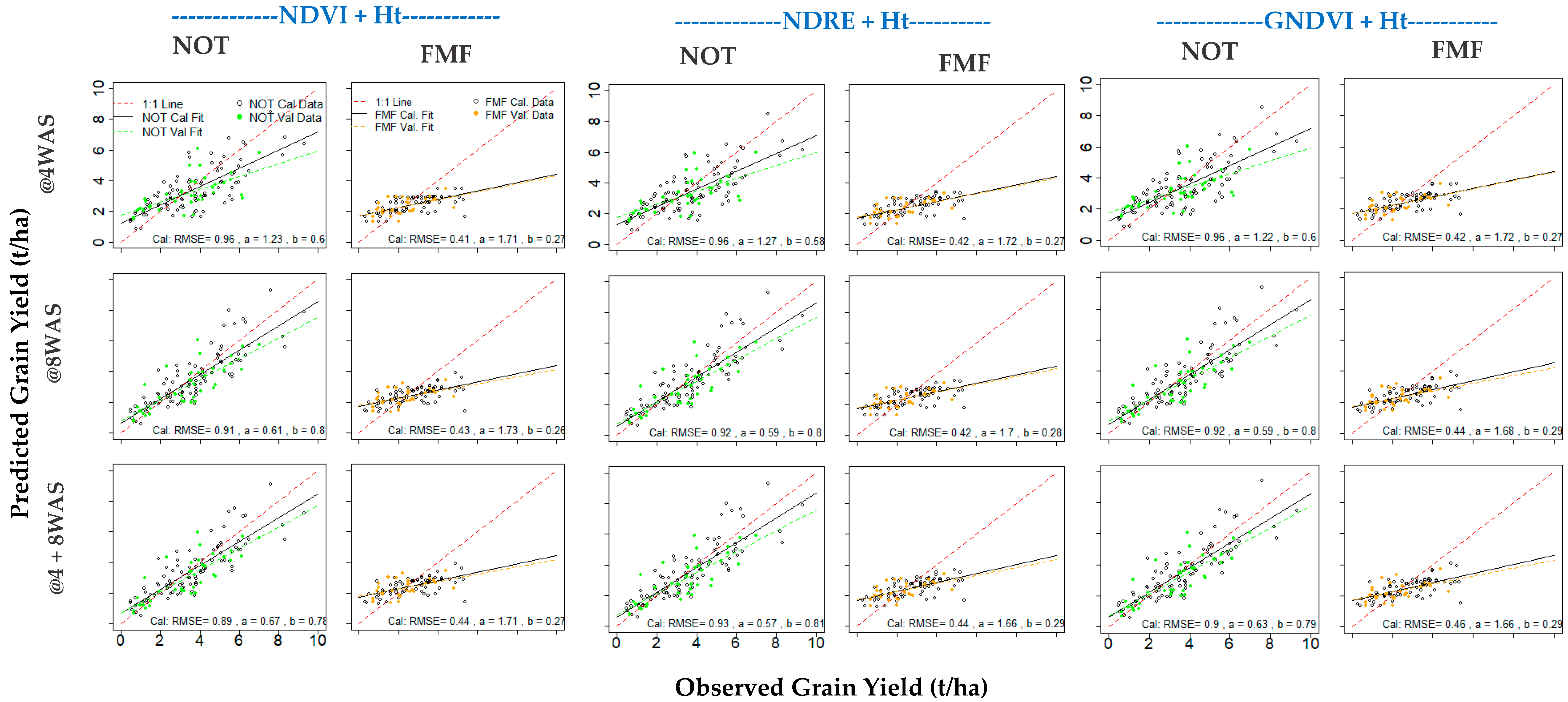
3.3. Predictability of Grain Yield Variability with(Out) Biophysical Variables

Relating grain yield to each VI separately, the highest explained yield variability at both growth stages were observed in NOTs (49% at 4WAS and 54% at 8WAS), compared to FMFs (42% at 4WAS) in the calibration dataset. The validation metrics (

Table 3. (a): Model performance metrics for maize grain yield prediction using UAV-derived vegetation indices (VI) with (out) inclusion of the measured biophysical variable, height (Ht) in multilocational nutrient omission trials (NOTs) near to farmers’ fields. (b): Model performance metrics for maize grain yield prediction using UAV-derived vegetation indices (VI), with(out) inclusion of the measured biophysical variable, height (Ht) in multilocational smallholder farmers’ fields.

(a)
	No-VI			NDVI		NDRE		GNDVI
		−Htǂ	+Ht	−Ht	+Ht	−Ht	+Ht	−Ht	+Ht
4WAS	a	-	1.73	2.41	1.75	2.81	1.74	2.35	1.73
	b	-	0.43	0.18	0.41	0.09	0.43	0.19	0.42
	r	-	0.65	0.43	0.63	0.23	0.65	0.43	0.64
	R2	-	0.41	0.16	0.38	0.03 ns	0.4	0.16	0.39
	RMSEP	-	0.21	0.38	0.23	0.29	0.21	0.4	0.23
8WAS	a	-	0.77	1.82	0.77	2.82	0.75	1.8	0.76
	b	-	0.69	0.29	0.68	0.09	0.69	0.33	0.68
	r	-	0.8	0.49	0.79	0.24	0.8	0.56	0.8
	R2	-	0.62	0.22	0.62	0.03 ns	0.63	0.29	0.62
	RMSEP	-	0.3	0.59	0.33	0.29	0.3	0.49	0.32
4 + 8WAS	a	-	0.8	1.84	0.67	2.8	0.75	1.8	0.69
	b	-	0.69	0.29	0.7	0.09	0.68	0.33	0.71
	r	-	0.8	0.5	0.81	0.23	0.79	0.55	0.81
	R2	-	0.63	0.23	0.64	0.03 ns	0.61	0.29	0.65
	RMSEP	-	0.3	0.57	0.35	0.29	0.32	0.49	0.3
(b)
	No-VI			NDVI		NDRE		GNDVI
		−Htǂ	+Ht	−Ht	+Ht	−Ht	+Ht	−Ht	+Ht
4WAS	a	-	1.74	1.73	1.73	1.75	1.75	1.71	1.71
	b	-	0.25	0.26	0.25	0.26	0.26	0.25	0.26
	r	-	0.53	0.53	0.54	0.52	0.53	0.54	0.53
	R2	-	0.26	0.26	0.26	0.24	0.25	0.26	0.25
	RMSEP	-	0.05	0.05	0.05	0.07	0.06	0.04	0.04
8WAS	a	-	1.75	1.75	1.79	1.75	1.75	1.73	1.74
	b	-	0.25	0.25	0.23	0.26	0.26	0.26	0.25
	r	-	0.53	0.53	0.49	0.52	0.51	0.54	0.51
	R2	-	0.25	0.25	0.21	0.24	0.23	0.26	0.24
	RMSEP	-	0.04	0.06	0.05	0.07	0.07	0.06	0.04
4 + 8WAS	a	-	1.74	1.75	1.77	1.72	1.74	1.7	1.71
	b	-	0.25	0.26	0.24	0.27	0.26	0.27	0.26
	r	-	0.53	0.52	0.49	0.53	0.53	0.54	0.5
	R2	-	0.25	0.24	0.21	0.25	0.25	0.26	0.23
	RMSEP	-	0.04	0.07	0.06	0.07	0.06	0.05	0.03

ns denotes non-significant at significance level, α, = 0.05; WAS denotes weeks after sowing; a is the model intercept, b is the slope, r is the correlation, Ht is plant height. Coefficient, R² is the adjusted coefficient of determination and RMSEP is the root mean square error of prediction. (a) ‡ Metrics of Null yield model without any explanatory variable: a = 2.80; b = 0.09; r = 0.24; R² = 0.03 ns; RMSEP = 0.30; (b) ‡ Metrics of Null model without any explanatory variable: a = 1.74; b = 0.25; r = 0.53; R² = 0.26; RMSEP = 0.05.

a,b) showed low yield predictability with UAV-derived VIs alone in both NOTs and FMFs. The maximum prediction of yield variability (r = 0.56; R² = 0.29) was achieved by fitting the mixed model with GNDVI values at 8WAS in NOTs (Table 3a). There was no meaningful improvement in assessed yield variability after merging VI data from both phenological stages (i.e., 4WAS + 8WAS) and analyzing them as time-series data for either NOT or FMF.

In NOTs, the results from the initial null model testing shows that the UAV-derived VIs are viable explanatory variables, considering that R² increases from 0.03 (null model) to the highest value of 0.29 (for GNDVI). In contrast, there was no improvement in the assessed yield variability across the FMFs, suggesting that the VIs are poor explanatory variables for yield variability. Further, the combination of measured Ht with each VI (Figure 7) showed that the predictability of grain yield at 4WAS and 8WAS increased significantly in NOTs (Table 3a) but not in FMFs (Table 3b). For instance, in NOTs, assessed variability of grain yield improved when NDRE was combined with Ht, with R² increasing from 0.03 to 0.63 (p < 0.001). Similarly, other VIs became better predictors of grain yield variability when combined with the Ht variable, with the R² value peaking at 0.64. The overall prediction error, RMSEP, mainly decreased (up to ~79%) after the inclusion of the height parameter, except when NDRE data for both growth stages were combined (Table 3a). In FMFs, the predictability of grain yield with VIs did not improve meaningfully (at 4WAS) after the inclusion of the Ht variable in each model run, but rather declined (~20%) at 8WAS, while the RMSEP values were stable, hovering around 0.03–0.07 at both of the growth stages that were assessed (Table 3b).

4. Discussion

4.1. Grain Yield Relationship with Measured Biophysical Variables

In this study, the set-up of NOTs next to farmers fields provided important context for the understanding of grain yield gap and predictability in smallholder farming systems. Our findings also have important ramification for agronomic decision support and aspirations for rapid (in-season) assessment of grain yield with UAV-derived data in farmers’ fields, especially in Africa. Across the multilocational NOT plots, the attainment of high yield (up to 9.3 t/ha) in plots where nutrient limitations are fully addressed, in contrast to control plots (where grain yield was as low as 0.49 t/ha), supports the notion that proper soil nutrient management can reduce the existing yield gap within the smallholder farming systems [4]. The availability of required nutrients for uptake at various growth stages of the maize crop affects overall plant development, including height, greenness, and canopy formation, which are represented by the measured biophysical variables (height, gNDVI, and percent canopy, respectively). The significant relationships assessed between grain yield and measured variables (mainly gNDVI and Ht) aligns with previous findings that support the selection of relevant proxies for rapid in-season assessment of yield variability [2,43]. However, the assessed relationships were weakly expressed (R² ≤ 0.17 and r ≤ 0.42), deviating from reported findings where strong relationships were established between maize grain yield and proximally-sensed biophysical variables in farmers’ fields, with R²-values typically greater than 0.5 (e.g., [43]). It should be noted that the relationship between yield and proxy variables can be influenced by artefacts of location-dependent soil nutrient conditions and environmental factors, such as short-term drought conditions. Such artefacts can negatively affect the final yield outcome by compromising plant vigor during the reproductive/grain-filling stages (before- and after−8WAS). In the study area, soil nutrient limitations and poor soil management practices are common [8,32], and we observed that the few farmers who applied nutrients predominantly adopt early growth stage application practice (mostly by surface dressing or broadcasting) without considering the high potential for rapid nutrient losses due to the sandy textural characteristics of the soil. This prevalent practice may explain the poor crop performance (lower yield) in farmers’ fields compared to NOTs where the nutrient management schedule included proper timings relative to growth stages and site conditions. More importantly, in FMFs, the expected waning-off of nutrient availability with plant growth bears potential implication for the usability of the UAV-acquired spectral information at two growth stages in this study. While earlier growth stages may have progressed well, with UAV-sensed spectral signals indicating the potential for realizable grain yield, nutrient deficiencies at later stages can alter reproductive processes and result in poor grain yields, thereby translating into a poor relationship between estimated grain yield and remotely-sensed spectral data. Further research exploration may be needed to unravel the effects of farmers’ nutrient management practices at various growth stages on yield predictability; however, this is beyond the scope of this article.

4.2. Nutrients, Not Genotype, May Influence UAV-Derived Vis-Insights from NOT

Within the multilocational NOTs, nutrient variations were more strongly expressed in the UAV-sensed VIs than genotype variations. Similar to other crops, maize genotypes are often released with the aim of improving resilience or tolerance to stress (such as drought and weed), and they consequently improve quality and quantity of yield outcomes. In some instances, such improvement may include modification of traits related to leaf morphology and canopy characteristics, to achieve desired responses to target stress conditions. Despite the expected difference in the phenotypic traits of different genotypes [44], the implementation of this study during the wet season (i.e., no drought stress), with full control of weeds in the experimental plots (i.e., no weed stress), may have addressed the major stresses that are likely to compromise the growth and development of the OPV genotype in this study. Therefore, in the absence of other stressors, soil nutrient status exerted a dominant effect on the overall yield outcomes for both OPV and Hybrid genotypes, without noticeable contrast. This is further supported by our observed data on percent canopy coverage (not reported), which showed that canopy coverage was similar within the OPV and Hybrid genotype plots at both of the growth stages evaluated. Because N and P are the most prevalent soil nutrient deficiencies within the savannah maize-based system of Nigeria [45,46], the application of appropriate fertilizer likely supported similar leaf formation and canopy morphology of maize stands across the plots, with no significant difference between genotypes. This suggests that the inherent genotype diversity in smallholder farming systems may not be a major concern for canopy-level light interception or reflectance that underlies the quality (including signal-noise ratio) of UAV-derived indices across (the complex mosaics of) farmers’ fields.

4.3. In-Season Grain Yield Variability Assessment with UAV-Derived VI: A Nuanced Outcome

The comparison of assessed grain yield variability between NOTs and FMFs unravels an often-neglected limitation to the applicability/transferability of agronomic predictive tools from experimental “controlled” conditions to usually “complex” farming systems. Despite the set-up of multilocational NOTs next to fields that were managed by smallholder farmers, we observed a strongly contrasting difference in the potential to assess grain yield variability based on UAV-derived VIs under both conditions. The observation that a combination of Ht with VIs improved the assessed grain yield variability in NOTs but not in FMFs contradicts our expectations that the biophysical variable will greatly improve outcomes for yield variability assessment, irrespective of the management condition. On the contrary, ground measured Ht (on a few stands within each farm) may not be universally useful to implement spatially explicit yield prediction within farmers’ fields, and seemingly requires further in-depth enquiry. However, UAV-derived canopy height data may be very relevant for spatially-explicit prediction of grain yield if the mounted sensor is properly calibrated (with ground control references) to provide reliable elevational/surface height (z) data. Field data collection in this study did not include instrumentation to calibrate the UAV-sensed surface model of the farms, thereby precluding the generation of gridded high-resolution height or elevation data. In agreement with Burke and Lobell [1], broadening the use of remotely-sensed imageries (including UAV-derived) for rapid yield assessment, especially across complex smallholder farmers’ fields, requires rigorous ground data for proper calibration of sensors and models. Arguably, an interplay of factors can also confound the usefulness of high-resolution UAV-derived VIs, including the aforementioned (amplified) noise that may be generated at the canopy level, especially in smallholder farming systems where canopy formation and structure are usually indeterminate across farms [2,34].

The grain yield variability explained by the UAV-derived VIs in FMFs (maximum of 42% in calibration and 26% in validation) is lower than previously reported in other studies that are based on ground-level proximate-sensing of crop fields over several time points throughout the growth and reproductive stages of the crop [12,21,43,47]. Recently, similar findings from complex farming systems in sub-Saharan Africa have been reported (e.g., [14]), where the explained maize yield variability hovered around 40%. It is probable that single (or sparse) time-step imageries are insufficient to fully elucidate in-season yield variability because growth processes that modulates final yield outcomes occur and can change at more frequent temporal scales between the time-points of imagery acquisition. Generally, VI imageries that are acquired during or close to the reproductive stages have been reported to be more suitable for yield assessment [28]. For instance, around 8WAS, the maize plants are closer to anthesis, and plant health at this stage is more likely to determine grain yield outcomes [33]. However, unanticipated environmental stress after anthesis can negatively impact the grain-filling process, with consequent implication for the final grain yield. The potential to achieve better predictability of grain yield by combining time series VIs from UAV-acquired imageries (e.g., at 4WAS + 8WAS) deserves further consideration. Our comparison of results between combined time-series data and single timestamp (especially at 8WAS) showed negligible or no improvement in the explained yield variability across farmers’ fields. Although this may obviate the suggestion that time-series imageries may improve yield forecasting in cropping systems [28], it aligns with idea that vegetation sensing should be implemented close to the most critical reproductive stage of the target crop [21,29,48,49]. In reality, justifying the additional costs associated with the acquisition of multiple/time-series imageries (time and resources for flights and analytics) may be contingent on gains in accuracy and a broader demand for agronomic decision support.

Notwithstanding the low predictability of grain yield in farmers’ fields, high resolution UAV-imageries are useful for the generation of agronomically relevant information about crop health and nutrient status in experimental plots and in farmers’ fields. For instance, the UAV-derived VIs distinctly showed major differences between plots based on nutrients and genotypes in NOTs (Figure 5), and this lends credence to the overall usefulness of UAV-derived VIs’ for the assessment of relative differences in nutrient status and overall crop health status in non-uniformly managed smallholder farming systems. We were unable to fully elucidate the other factors that may account for yield variability across the farmer managed fields compared to NOTs due to incomplete information from the volunteer farmers. Although the farmers agreed to grant access for data collection and provided basic information on approximate sowing date, they were unavailable and unwilling to document actual tending operations (such as weeding, type and quantity of fertilizer, organic manure application, genotype, etc.). Future study on complex farming systems should include careful assessment of these potential factors.

5. Conclusions

Successful acquisition of quality high-resolution imageries and processing of the agronomically-relevant vegetation indices is an important step towards understanding within-and between-farm variability of yield and related indicators at the field-scale. This study provides further insight into the potential use of UAV-derived vegetational indices to assess yield variability for rapid agronomic monitoring and robust decision-support in smallholder farming systems. By setting up multilocational nutrient omission trials close to several farmers’ fields, our findings showed that nutrients, not genotype, significantly explained the observed yield variability. The weak predictability of maize grain yield variability based on selected indices (NDVI, NDRE, and GNDVI) indicates a lingering gap in UAV application for rapid yield assessment within complex smallholder farming systems beyond experimental conditions and large-scale (mono-cropped) field conditions. Because the combination of UAV-derived VIs with the ground-measured biophysical variable (mainly height) improved assessed yield variability in NOTs but not in FMFs, we believe that VIs acquired at only two timesteps do not provide a sufficient basis to reliably predict grain yield within farmers’ fields. However, it is advantageous that the UAV-based sensing of croplands can generate continuous high-resolution canopy height data that may be useful for spatially-explicit relative yield prediction, contingent on accurate calibration. While the demand for in-season prediction of crop yield in smallholder farming systems remains topical, especially between- and within-fields, further explorations of UAV application should consider and account for potential confounding factors in farmers’ fields (such as nutrient application regimes, soil characteristics, and planting density), which can vary between farms and influence canopy formation, light interception, and spectral reflectance at various stages of growth.

References

1. Burke, M.; Lobell, D.B. Satellite-based assessment of yield variation and its determinants in smallholder African systems. Proc. Natl. Acad. Sci. USA 2017, 114, 2189–2194. [Google Scholar] [CrossRef] [Green Version]
2. Tittonell, P.; Vanlauwe, B.; Leffelaar, P.; Giller, K. Estimating yields of tropical maize genotypes from non-destructive, on-farm plant morphological measurements. Agric. Ecosyst. Environ. 2005, 105, 213–220. [Google Scholar] [CrossRef]
3. Herbert, B. Land use efficiency under maize-based cropping system in Zaria, Nigeria. J. Agric. For. Soc. Sci. 2005, 3, 114–120. [Google Scholar]
4. Giller, K.E.; Tittonell, P.; Rufino, M.; Van Wijk, M.; Zingore, S.; Mapfumo, P.; Adjei-Nsiah, S.; Herrero, M.; Chikowo, R.; Corbeels, M.; et al. Communicating complexity: Integrated assessment of trade-offs concerning soil fertility management within African farming systems to support innovation and development. Agric. Syst. 2011, 104, 191–203. [Google Scholar] [CrossRef]
5. Onuk, E.G.; Alimba, J.O.; Kasali, R.A. Comparative Study of Production Efficiencies Under Cowpea-Maize and Groundnut- Millet Intercropping Systems in The North Central Zone, Nigeria. Prod. Agric. Technol. 2015, 11, 108–121. [Google Scholar]
6. Vanlauwe, B.; Coe, R.; Giller, K.E. Beyond Averages: New Approaches to Understand Heterogeneity and Risk of Technology Success or Failure in Smallholder Farming. Exp. Agric. 2019, 55, 84–106. [Google Scholar] [CrossRef] [Green Version]
7. Nagy, J.G.; Edun, O. Assessment of Nigerian Government Fertilizer Policy and Suggested Alternative Market-Friendly Policies; Report to International Fertilizer Development Corporation; IFDC: Muscle Shoals, AL, USA, 2002; 67p. [Google Scholar]
8. Olarinde, L.O.; Manyong, V.M.; Akintole, J.O. Attitudes towards risk among maize farmers in the dry savanna zone of Nigeria: Some prospective policies for improving food production. Afr. J. Agric. Res. 2007, 2, 399–408. [Google Scholar]
9. Efron, S. The Use of Unmanned Aerial Systems for Agriculture in Africa: Can it Fly? Master’s Thesis, Pardee Rand Graduate School, Santa Monica, CA, USA, 2015; 369p. Available online: https://www.rand.org/content/dam/rand/pubs/rgs_dissertations/RGSD300/RGSD359/RAND_RGSD359.pdf (accessed on 9 July 2017).
10. Hall, O. The Challenge of Comparing Crop Imagery over Space and Time. ICT Update 2016, 82:14. Available online: http://ictupdate.cta.int (accessed on 9 July 2017).
11. Yang, G.; Liu, J.; Zhao, C.; Li, Z.; Huang, Y.; Yu, H.; Xu, B.; Yang, X.; Zhu, D.; Zhang, X.; et al. Unmanned Aerial Vehicle Remote Sensing for Field-Based Crop Phenotyping: Current Status and Perspectives. Front. Plant Sci. 2017, 8, 1111. [Google Scholar] [CrossRef]
12. Benincasa, P.; Antognelli, S.; Brunetti, L.; Fabbri, C.A.; Natale, A.; Sartoretti, V.; Modeo, G.; Guiducci, M.; Tei, F.; Vizzari, M. Reliability of NDVI derived by high resolution satellite and UAV compared to in-field methods for the evaluation of early crop n status and grain yield in wheat. Exp. Agric. 2018, 54, 604–622. [Google Scholar] [CrossRef]
13. Zhang, C.; Walters, D.; Kovacs, J.M. Applications of Low Altitude Remote Sensing in Agriculture upon Farmers’ Requests—A Case Study in Northeastern Ontario, Canada. PLoS ONE 2014, 9, e112894. [Google Scholar] [CrossRef]
14. Wahab, I.; Hall, O.; Jirström, M. Remote Sensing of Yields: Application of UAV Imagery-Derived NDVI for Estimating Maize Vigor and Yields in Complex Farming Systems in Sub-Saharan Africa. Drones 2018, 2, 28. [Google Scholar] [CrossRef] [Green Version]
15. Song, Y. Evaluation of the UAV-BASED Multispectral Imagery and Its Application for Crop Intra-Field Nitrogen Monitoring and Yield Prediction in Ontario. Master’s. Thesis, The University of Western Ontario, London, ON, Canada, 2016. Paper 4085. [Google Scholar]
16. Nebiker, S.; Lack, N.; Abächerli, M.; Läderach, S. Light-Weight Multispectral UAV Sensors and their capabilities for predicting grain yield and detecting plant diseases. ISPRS Int. Arch. Photogramm. Remote Sens. Spat. Inf. Sci. 2016, 963–970. [Google Scholar] [CrossRef]
17. Salamí, E.; Barrado, C.; Pastor, E. UAV Flight Experiments Applied to the Remote Sensing of Vegetated Areas. Remote. Sens. 2014, 6, 11051–11081. [Google Scholar] [CrossRef] [Green Version]
18. Tucker, C.J. Red and photographic infrared linear combinations for monitoring vegetation. Remote. Sens. Environ. 1979, 8, 127–150. [Google Scholar] [CrossRef] [Green Version]
19. Huete, A.; Didan, K.; Miura, T.; Rodriguez, E.P.; Gao, X.; Ferreira, L.G. Overview of the radiometric and biophysical performance of the MODIS vegetation indices. Remote Sens. Environ. 2002, 83, 195–213. [Google Scholar] [CrossRef]
20. Haghighattalab, A.; González Pérez, L.; Mondal, S.; Singh, D.; Schinstock, D.; Rutkoski, J.; Ortiz-Monasterio, J.I.; Singh, R.P.; Goodin, D.; Poland, J.A. Application of unmanned aerial systems for high throughput phenotyping of large wheat breeding nurseries. Plant Methods 2016, 12, 1–15. [Google Scholar] [CrossRef] [Green Version]
21. Maresma, Á.; Ariza, M.; Martínez, E.; Lloveras, J.; Martínez-Casasnovas, J.A. Analysis of Vegetation Indices to Determine Nitrogen Application and Yield Prediction in Maize (Zea mays L.) from a Standard UAV Service. Remote. Sens. 2016, 8, 973. [Google Scholar] [CrossRef] [Green Version]
22. Vega, F.A.; Ramirez, F.C.; Saiz, M.P.; Rosua, F.O. Multi-temporal imaging using an unmanned aerial vehicle for monitoring of sunflower crop. Biosyst. Eng. 2015, 132, 19–27. [Google Scholar] [CrossRef]
23. Gitelson, A.A.; Viña, A.; Ciganda, V.; Rundquist, D.C.; Arkebauer, T.J. Remote estimation of canopy chlorophyll content in crops. Geophys. Res. Lett. 2005, 32, 32. [Google Scholar] [CrossRef] [Green Version]
24. Nguy-Robertson, A.; Gitelson, A.A.; Peng, Y.; Viña, A.; Arkebauer, T.; Rundquist, D. Green Leaf Area Index Estimation in Maize and Soybean: Combining Vegetation Indices to Achieve Maximal Sensitivity. Agron. J. 2012, 104, 1336–1347. [Google Scholar] [CrossRef] [Green Version]
25. Gu, Y.; Wylie, B.K.; Howard, D.M.; Phuyal, K.P.; Ji, L. NDVI saturation adjustment: A new approach for improving cropland performance estimates in the Greater Platte River Basin, USA. Ecol. Indic. 2013, 30, 1–6. [Google Scholar] [CrossRef]
26. Isla, R.; Quílez, D.; Valentín, F.; Casterad, M.A.; Aibar, J.; Maturano, M. Utilización de imágenes aéreas multiespectrales para evaluar la disponibilidad de nitrógeno en maíz (Use of multispectral airbone images to assess nitrogen availability in maize). In Teledetección, Bosques y Cambio Climático; Recondo, C., Pendás, E., Eds.; Asociación Española de Teledetección: Mieres, Spain, 2011; pp. 9–12. [Google Scholar]
27. Watanabe, K.; Guo, W.; Arai, K.; Takanashi, H.; Kajiya-Kanegae, H.; Kobayashi, M.; Yano, K.; Tokunaga, T.; Fujiwara, T.; Tsutsumi, N.; et al. High-Throughput Phenotyping of Sorghum Plant Height Using an Unmanned Aerial Vehicle and Its Application to Genomic Prediction Modeling. Front. Plant Sci. 2017, 8, 421. [Google Scholar] [CrossRef] [Green Version]
28. Schut, A.G.T.; Traore, P.C.S.; Blaes, X.; De By, R.A. Assessing yield and fertilizer response in heterogeneous smallholder fields with UAVs and satellites. Field Crop. Res. 2018, 221, 98–107. [Google Scholar] [CrossRef]
29. Sakamoto, T.; Gitelson, A.A.; Arkebauer, T.J. Near real-time prediction of U.S. corn yields based on time-series MODIS data. Remote. Sens. Environ. 2014, 147, 219–231. [Google Scholar] [CrossRef]
30. Yang, B.; Hawthorne, T.L.; Torres, H.; Feinman, M. Using Object-Oriented Classification for Coastal Management in the East Central Coast of Florida: A Quantitative Comparison between UAV, Satellite, and Aerial Data. Drones 2019, 3, 60. [Google Scholar] [CrossRef] [Green Version]
31. Sibley, A.M.; Grassini, P.; Thomas, N.E.; Cassman, K.G.; Lobell, D.B. Testing Remote Sensing Approaches for Assessing Yield Variability among Maize Fields. Agron. J. 2013, 106, 24–32. [Google Scholar] [CrossRef]
32. Shehu, B.M.; Merckx, R.; Jibrin, J.M.; Kamara, A.Y.; Rurinda, J. Quantifying Variability in Maize Yield Response to Nutrient Applications in the Northern Nigerian Savanna. Agronomy 2018, 8, 18. [Google Scholar] [CrossRef] [Green Version]
33. Ritchie, S.W.; Hanway, J.J.; Benson, G.O. How a Corn Plant Develops; Special Report 48 (Revised); Iowa State University of Science and Technology Cooperative Extension Service: Ames, IA, USA, 1966; Available online: https://s10.lite.msu.edu/res/msu/botonl/b_online/library/maize/www.ag.iastate.edu/departments/agronomy/corngrows.html#management (accessed on 23 March 2016).
34. Geipel, J.; Link, J.; Claupein, W. Combined Spectral and Spatial Modeling of Corn Yield Based on Aerial Images and Crop Surface Models Acquired with an Unmanned Aircraft System. Remote. Sens. 2014, 6, 10335–10355. [Google Scholar] [CrossRef] [Green Version]
35. Cammarano, D.; Fitzgerald, G.J.; Casa, R.; Basso, B. Assessing the Robustness of Vegetation Indices to Estimate Wheat N in Mediterranean Environments. Remote. Sens. 2014, 6, 2827–2844. [Google Scholar] [CrossRef] [Green Version]
36. Hatfield, J.L.; Prueger, J.H. Value of Using Different Vegetative Indices to Quantify Agricultural Crop Characteristics at Different Growth Stages under Varying Management Practices. Remote. Sens. 2010, 2, 562–578. [Google Scholar] [CrossRef] [Green Version]
37. Viña, A.; Gitelson, A.A.; Nguy-Robertson, A.L.; Peng, Y. Comparison of different vegetation indices for the remote assessment of green leaf area index of crops. Remote. Sens. Environ. 2011, 115, 3468–3478. [Google Scholar] [CrossRef]
38. Xue, J.; Su, B. Significant Remote Sensing Vegetation Indices: A Review of Developments and Applications. J. Sensors 2017, 2017, 1–17. [Google Scholar] [CrossRef] [Green Version]
39. Carletto, C.; Jolliffe, D.; Banerjee, R. From Tragedy to Renaissance: Improving Agricultural Data for Better Policies. J. Dev. Stud. 2015, 51, 133–148. [Google Scholar] [CrossRef]
40. Nziguheba, G.; Tossah, B.K.; Diels, J.; Franke, A.C.; Aihou, K.; Iwuafor, E.N.O.; Nwoke, C.; Merckx, R. Assessment of nutrient deficiencies in maize in nutrient omission trials and long-term field experiments in the West African Savanna. Plant Soil 2009, 314, 143–157. [Google Scholar] [CrossRef]
41. Patrignani, A.; Ochsner, T.E. Canopeo: A Powerful New Tool for Measuring Fractional Green Canopy Cover. Agron. J. 2015, 107, 2312–2320. [Google Scholar] [CrossRef] [Green Version]
42. Hijmans, R.J.; van Etten, J.; Cheng, J.; Mattiuzzi, M.; Summer, M.; Greenber, J.A.; Baston, D.; Bevan, A.; Bivand, R.; Busseto, L.; et al. Geographic Data Analysis and Modeling: Package Raster. 2016. Available online: https://cran.r-project.org/web/packages/raster/raster.pdf (accessed on 2 September 2017).
43. Tagarakis, A.C.; Ketterings, Q.M. In-Season Estimation of Corn Yield Potential Using Proximal Sensing. Agron. J. 2017, 109, 1323–1330. [Google Scholar] [CrossRef] [Green Version]
44. Makanza, R.; Zaman-Allah, M.; Cairns, J.E.; Magorokosho, C.; Tarekegne, A.; Olsen, M.; Prasanna, B.M. High-Throughput Phenotyping of Canopy Cover and Senescence in Maize Field Trials Using Aerial Digital Canopy Imaging. Remote. Sens. 2018, 10, 330. [Google Scholar] [CrossRef] [Green Version]
45. Carsky, R.J.; Nokoe, S.; Lagoke, S.T.O.; Kim, S.K. Maize yield determinants in farmer-managed trials in the Nigerian Northern Guinea savanna. Exp. Agric. 1998, 34, 407–422. [Google Scholar] [CrossRef]
46. Hartmann, L.; Gabriel, M.; Zhou, Y.; Sponholz, B.; Thiemeyer, H. Soil Assessment along Toposequences in Rural Northern Nigeria: A Geomedical Approach. Appl. Environ. Soil Sci. 2014, 2014, 628024. [Google Scholar] [CrossRef]
47. Tagarakis, A.C.; Ketterings, Q.M.; Lyons, S.; Godwin, G. Proximal Sensing to Estimate Yield of Brown Midrib Forage Sorghum. Agron. J. 2017, 109, 107–114. [Google Scholar] [CrossRef] [Green Version]
48. Teal, R.K.; Tubana, B.; Girma, K.; Freeman, K.W.; Arnall, D.B.; Walsh, O.; Raun, W. In-Season Prediction of Corn Grain Yield Potential Using Normalized Difference Vegetation Index. Agron. J. 2006, 98, 1488–1494. [Google Scholar] [CrossRef] [Green Version]
49. Cao, J.; Leng, W.; Liu, K.; Liu, L.; He, Z.; Zhu, Y. Object-Based Mangrove Species Classification Using Unmanned Aerial Vehicle Hyperspectral Images and Digital Surface Models. Remote. Sens. 2018, 10, 89. [Google Scholar] [CrossRef] [Green Version]
Figure 1. Map showing the multiple locations of the farmers’ fields and nutrient omission trials (NOTs) that were covered by unmanned air vehicle (UAV) flight missions and included in this study.
Agronomy 10 01934 g001
Figure 2. Frequency of estimated maize grain yield in smallholder farms across multilocational nutrient omission trials (NOTs) and farmer managed fields (FMF).
Agronomy 10 01934 g002
Figure 3. Ground measured normalized difference vegetation index (NDVI), plant height (Ht), and percent canopy cover (CC) of maize in smallholder farms imposed with different nutrient treatment conditions under multilocational and widely distributed nutrient omission trials (NOTs). At 4 weeks after sewing (WAS) (orange boxplots), the nutrient treatment effect was not evident, but significantly higher effects of NP, NPK, and NPK+ were observed at 8WAS (green box plots). CTR = Control, N = Nitrogen, P = Phosphorus, K = Potassium, and + denotes addition of micronutrients. The horizontal line on each boxplots shows mean value, and the whiskers indicate the 95% confidence interval.
Agronomy 10 01934 g003
Figure 4. Linear relationship between maize grain yield and measured normalized difference vegetation index (gNDVI), plant height, and canopy cover percentage measured on nutrient omission trials (NOTs) within smallholder maize farms in Nigeria. Regression lines are included for only significant relationshipsand assessed by the coefficient of determination, R-sq (at significance level, α, = 0.05); WAS denotes Weeks after Sowing.
Agronomy 10 01934 g004
Figure 5. Vegetation indices (VIs) derived from UAV-sensed multispectral imageries, covering maize plots within nutrient omission trials (NOTs) and farmers’ fields at Bunkure, Kano. The grey imagery shows red-edge reflectance band acquired at 8 weeks after sowing (WAS), while the colored imageries show the VIs at 4 and 8WAS.
Agronomy 10 01934 g005
Figure 6. Nutrient-induced variation of UAV-derived vegetation indices (VIs) within multilocational nutrient omission trials (NOTs) in smallholder maize farming systems at 8 weeks after sowing. NDVI denotes Normalized difference VI, NDRE is Normalized difference red-edge, and GNDVI is green normalized difference VI. * and ** denotes outlier data points in the boxplot.
Agronomy 10 01934 g006
Figure 7. Relationship between observed and predicted maize grain yield based on fitted linear mixed effect model using and UAV-derived Vegetation Indices (VIs) combined with plant height (Ht) data from multilocation smallholder maize farms in Nigeria. NOT = Nutrient omission trials; FMF = Farmer managed fields; WAS = Weeks after sowing; a = Intercept; b = Slope estimate; Calibration (Cal) metrics are shown on the charts and additional Validation (Val) metrics are presented in Table 3a,b.
Agronomy 10 01934 g007