3. Bayesian Network Learning Model
Bayesian networks (BNs), also known as belief networks, are directed acyclic graphical (DAG) probabilistic models that are widely used to represent the complex joint probability distributions between network variables. The complex causal relationships between random variables
are split into multiple local distributions and represented as a DAG. Independent random variables within a DAG are represented as nodes. They are linked by edges from the direct causes as determined by the conditional dependencies probability
P. Each variable is conditionally dependent on its effects and independent of its non-effects. Conditional dependencies can be estimated either by using statistical and computational methods or incorporation of expert experience. Let
X denoted as a set of random variables in a DAG, then the full joint probability distribution has expressed as:
where
and
,
, are child and parent nodes, respectively. The distribution of child nodes depends only on their parent nodes, the number of which is limited. The global joint distribution is split into local distributions. The forecast model was coded and implemented using the statistical programming language R (version 3.4.2) making use of validated, open-source algorithm libraries: bnlearn (structure learning), mltool (calculating MSE), and other plotting packages (i.e., Rgraphviz, graph, plot3D, ggplot2, RColorBrewer).
3.1. Supervised and Algorithm Learning
Fitting a Bayesian network to data, usually called learning has two forms: structural learning and inference learning. Structural learning also has various forms, and can be based on expert knowledge, termed supervised learning, or based on statistical or computational learning algorithms, termed algorithmic learning. This later approach uses multiple learning algorithms to link random variables within a network into a DAG. Random variables within a network can be discrete, continuous, or hybrid data types, where hybrid is a network containing both discrete and continuous random variables. In a hybrid Bayesian network, network learning to establish causal relationships proceeds under certain restrictions: a child of continuous data type can have either discrete or continuous data type parent nodes, but a child of discrete data type must have discrete parent nodes. This logical connection between child and parent nodes helps to avoid linking problems in structure learning, providing better estimations for parameter learning.
Both supervised and algorithmic learned were employed for the Bayesian network to learn the complex interactions between a grapevine and PM disease under varying environmental conditions. For the supervised learning, the causal relationships within the Bayesian network were linked to the calibrated empirically-derived equations described previously in
Section 2.3 and
Section 2.4.
The grape PM risk assessment model,
[
21], was used to specify airborne conidium concentration for structural learning of the model. This model is developed from the Richards model using CGDD based on a
threshold. The Richards model was selected because it had used the observations from the same experimental farm site in this study, which was responsible for reducing fungicide spray for disease control by as much as 40% from 2004 to 2007. We examined the Pearson correlations between the DI for the three susceptible grape cultivars. The PM risk assessment model had different base temperatures ranging from
to
. A temperature of
was selected as the base temperature because it had the highest value in the correlations. The PM risk assessment model is:
where
is the cumulative growing degree days from Equation (
1).
Numerous approaches exist for implementing algorithm learning, with the two main approaches being constraint-based and score-based learning. Constraint-based learning involves developing relationships based on the framework from [
39], which uses a conditional independence test inductive causation (IC) to learn the Bayesian network structure. Structural learning involves determining the so-called Markov blanket of each node in the network and is defined as containing the only knowledge needed to predict the behavior of a node and its children within a larger network. Learning algorithms include the Grow-Shrink (GS) [
40], the Incremental Association (IAMB) [
41], the Fast Incremental Association (Fast-IAMB) [
42], and the Interleaved Incremental Association (Inter-IAMB) [
41]. In score-based learning, a network is learned from the network’s best goodness of fit by assigning a network score from the application of a general heuristic optimization technique to each candidate network. A commonly-used example of a score-based learning algorithm, for example, Hill-Climbing (HC), learns a network structure using a step progress process. In HC learning, a graphical score is computed for a randomly assigned network structure as a network score at the beginning of the process. A new score is computed from the assigned network structure by adding, deleting, or reversing an arc’s direction one at a time. The new graphical score will become the network score if it has a higher value than the previous one. The process of the computation repeats again and again until the network score reaches to its maximum. The corresponding network structure, which has the maximum network score, has the best goodness of fit to the network data. HC is chosen as the algorithm learning approach in this study because of its flexibility and power to handle the hybrid data types existing in our network data. To enhance the robustness of the network structure generated from score-based causal relationships between child and parents sets, a bootstrap sampling technique with an iteration of 5000 is performed, and two criteria—conditional dependence strength of above 80% and arc directions appearing in more than 50% of the iterations—are applied to the HC structure learning.
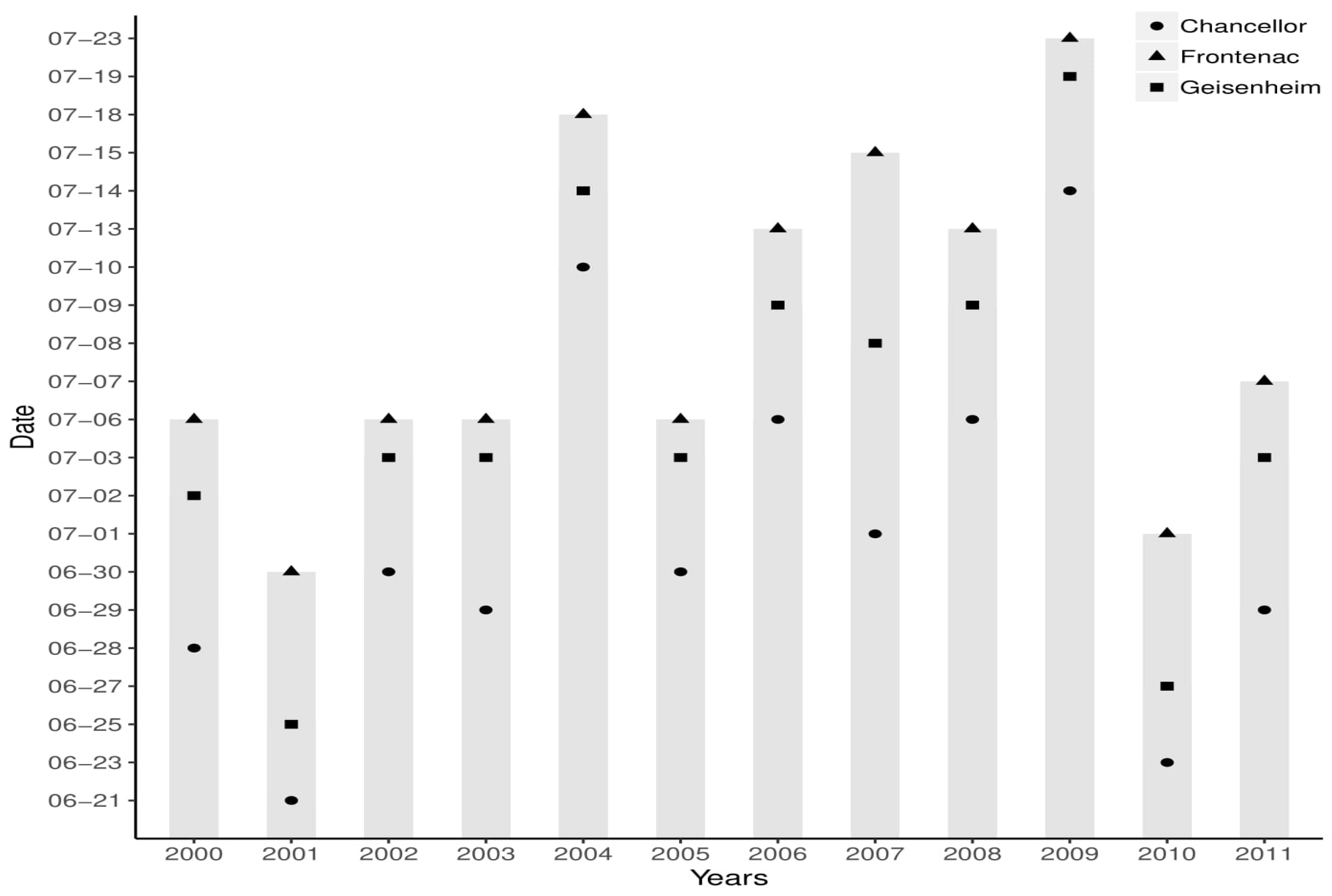
The first disease infection likely occurs between the end of June and July, which is during the flowering stage of the grape (
Figure 3). Establishing the initial modeling date is important because this can influence the model accuracy of disease risk. Modeling results were examined for four selected starting dates to determine the best date for initial disease risk modeling. These dates were selected under different assumptions: (1) the flowering date as the time of primary infection onset; (2) the mid-flowering date as the likely onset of secondary infection; (3) July 1st when the infection spreads to other plants, and (4) using the actual observed date of infection start as the estimated model start date may improve disease risk predictions. At the beginning of each growing season (1 April), the timing of the grapevine growing and mid-flowering stages were also estimated by the CGDD index (Equation (
1)) using daily mean temperature. The estimation of the PM growth factor is based on selected dates using Equations presented in
Section 2.4 and are specified for both the supervised and algorithm learning.
Table 2 summarizes the random variables used for network learning, including the additional considered day-to-day variability of relative humidity. Bayesian network modeling in both supervised and algorithm modes are trained for the three susceptible grape cultivars using observational data from 2000 to 2010 and then tested against actual pathogen occurrence and progression in 2011. Model forecast accuracy was evaluated comparing supervised and algorithm learning and a range of starting dates. The best-performing model was then used to examine the forecast performance and optimal forecast window length using GEFS input data.
3.2. Forecast Skill under Different Learning Modes
The performance of the forecast model under supervised and algorithm learning was evaluated and inter-compared using: (1) model skill in goodness-of-fit testing, which examined how well the model worked in accurately reproducing training data; and (2) model performance in prediction, providing benchmark information about model accuracy using forecast weather data. The learned model structure identified a subset of random variables listed in
Table 2. Random variables in a subset were selected by removing one or more unclear but considerable factors: the degree-days based assessment model (Pmaxacc), relative humidity (RH), and plant stages (PS) one at a time from the full data. A total of eight cases were examined: Case 1, full data; Case 2, remove RH; Case 3, remove PS; Case 4, remove Pmaxacc; Case 5, remove PS and RH; Case 6, remove RH and Pmaxacc; Case 7, remove PS and Pmaxacc; and Case 8, remove PS, Pmaxacc, and RH. Over-learning or over-fitting is a common problem in parameter learning, in which the network model is forced to accommodate data or parameters that do not contribute information; this results in degraded model predictive skill.
k-fold cross-validation, where
k is the number of years in the training data, has been applied to prevent over-learning. In this approach mean-absolute-error (MAE) and root-mean-squared-error (RMSE) are used as metrics to identify prediction bias and for variance comparison. Metrics used for model skill comparison for prediction results similarly include the MAE and RMSE generated for the 2011 growing season.
Cross-validation using the
k-fold method is a re-sampling technique often used to evaluate the prediction performance of a machine learning model using limited data sample as training data. In
k-fold cross-validation, the training data are split into
k subsets of equal size which are used to assess how the omission of one subset affects the learning of a Bayesian network from the rest of the subsets, by generating model predictions for the omitted subset. In this study, the training data set were split into k subsets by years. A single year is randomly removed to act as testing data, and the rest of the data are used for parameter learning using both supervised and algorithm learning approaches. The corresponding results of bias (MAE) and variance (RMSE) loss functions can be applied to measure deviation and discrepancy, separately, to determine how close model predictions were to the actual outcomes. Both MAE and RMSE can be defines as:
where
is the residual or error between the model predictions and the actual values. A lower value of MAE and RMSE indicates a model exhibiting better performance.
4. Model Forecast Evaluation
Sensitivity analysis (i.e., for a static or time-independent model) involves varying input variables, typically one at a time, to measure how it impacts a model’s output. Scenario analysis involves varying input variables to measure its impact on a future value either as future model predictions (if internally forced), or as projections (if externally forced). In the context of dynamic or time-dependent (i.e., forecast) models, shifting an input (e.g., climate or weather input variable) that is time-dependent generates variation over time. Furthermore, when forecast models have cumulative variables or interactions between multiple variables, future model outcomes can also become dependent and coupled across time. In such cases, sensitivity and scenario analysis becomes more integrated and less independently defined.
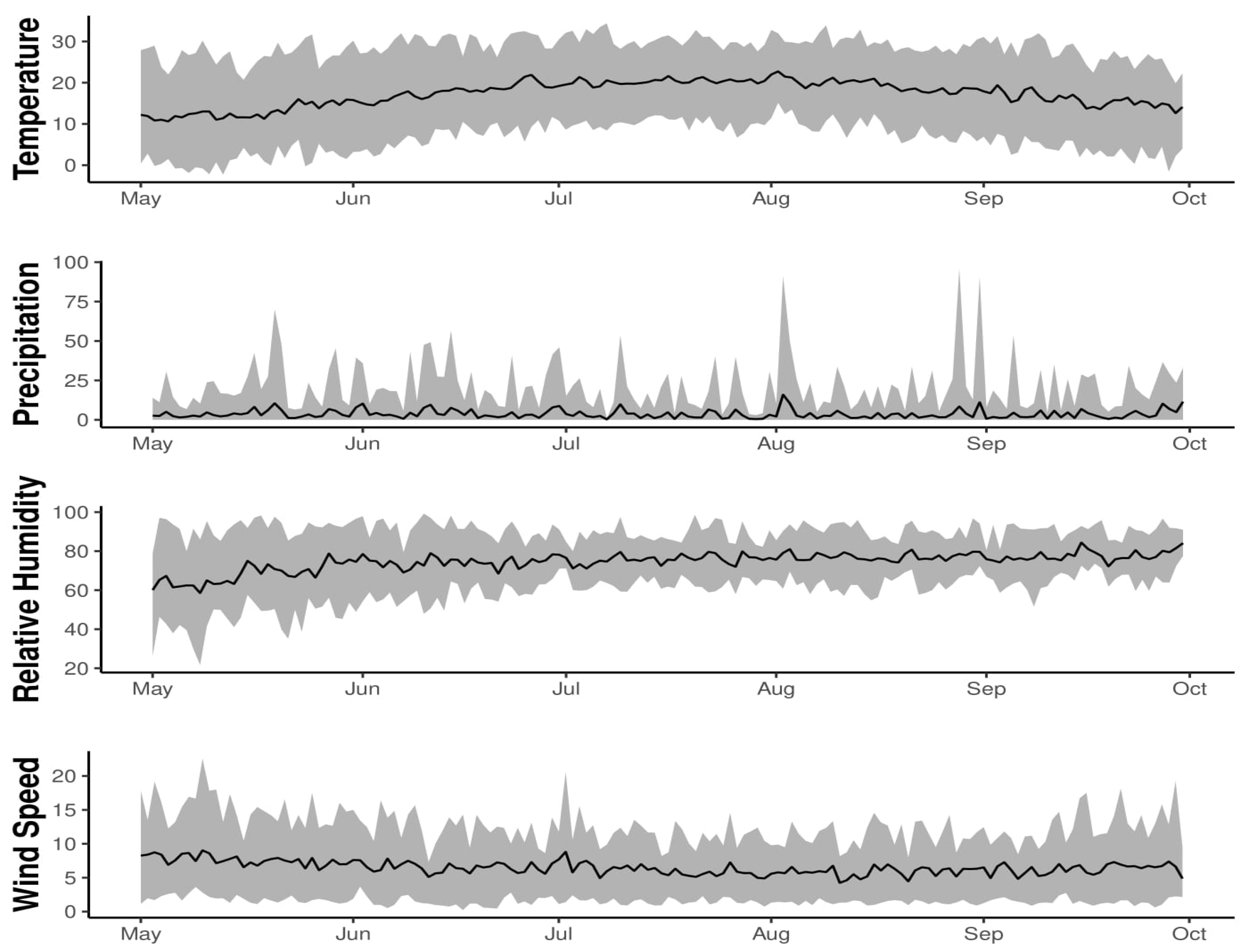
To understand the effect of a warmer and colder climate on DI model forecasts for the three northern cultivars, we varied the input daily mean temperature by in 2011. The runs with warmer and colder temperature were referred to as warm and cold year scenarios, respectively, and compared to the actual or baseline temperature at the study site in 2011. We also varied the model’s forecasting window length from 1, out to 16 days, to assess how robust the model’s forecasts of DI are over time, how sensitive its error is to the length of the forecasting window, and evaluate the GEFS reforecasted weather data as a model input for generating forecasts out to 16 days in advance. This analysis involved comparing the model’s forecast error statistics (MAE and RMSE) over time (days). The Bayesian network model with supervised learning, was used with GEFS reforecasted weather data for climate/weather variable input. Starting 1 April 2011, host plant stages were estimated using historical weather data and used to identify the mid-flowering date (2 July) to initiate the forecast model. Canopy-height daily maximum/minimum temperature, total precipitation, air pressure, specific humidity, and U/V component of wind were selected. Scalar mean daily wind speed was computed using the U/V-component wind variables. The daily mean temperature was calculated as the mean of the daily maximum and minimum temperature. The relative humidity was calculated from specific humidity using daily mean temperature and air pressure as inputs to the statistical R programming function from the "humidity R package". Weather data was averaged from 11 ensembles and used as model inputs for DI forecasting at a 16-day window. For each day after 2 July, the calibration of the Bayesian network model was performed using historical data from 1 April up to the present day and used for DI forecasting using data generated from GEFS.
6. Results
The performance of the forecast model was evaluated by varying the starting date (i.e., 4 selected starting dates) using a subset of variables (
Table 3). After determining the best model starting date (i.e., first disease date) simulation runs using 8 different variable subsets were performed (
Table 4). These tables provide a summary of the resulting mean-absolute-error (MAE) and root-mean-squared-error (RMSE) validation metrics for the northern grape cultivars. The forecast model was trained using data from 2000–2010 and validated using data for 2011.
Model forecast skill was evaluated based on k-fold validation statistics (MAE, RMSE) across the years 2000–2011 which removes k years at a time from the data and re-assesses forecast skill. The model was also validated by training the model on all of the historical data (2000–2010) (i.e., removing only data for year 2011) and then comparing its forecasts against 2011 data. Smaller values in both MAE and RMSE indicate higher forecast skill.
For supervised learning, the optimal initial date for start disease risk prediction was starting from first disease date in Case 1, containing all the network variables in the modeling structure. This run had the smallest values of cross-validated RMSE and predictive error in 2011 (MAE and RMSE). The smallest value of MAE (1.83) for training data was in Case 6 with model initialed from the flowering date but with higher values in RMSE for training data and MAE and RMSE for prediction data in the first disease date. The highest values of MAE and RMSE in both training and prediction data were from Mid-Flowering data with Case 6, which do not include relative humidity and degree-days based risk assessment model in the model structure.
In algorithm learning, Cases 2 and 3 performed the best, which did not contain relative humidity or plant stage. The best model performance was from the first disease date in Case 2 that had the smallest values of MAE and RMSE in both cross-validation and prediction. The highest values of cross-validated MAE (3.9) and RMSE (6.13) were for flowering date in Case 2, which had small MAE (0.57) and RMSE (0.99), as with the first disease date. The highest MAE and RMSE values in prediction was for flowering, which had high values of MAE and RMSE similar to mid-flowering. In general, cross-validated MAE and RMSE values were higher than the prediction values of these metrics in historical drought years of 2000, 2002, and 2008. Model accuracy of disease prediction was also evaluated with and without drought conditions, by adding a binary factor identifying historical years of drought (2000, 2002, 2008). The best performing model for supervised learning with drought years factor being Case 3 with model initialed from the first disease date, which has MAE and RMSE of 2.36 and 4.16 from training data and 1.13 and 1.52 from predictions, respectively. The best performing network structure in algorithm learning being Case 2 from the first disease date which has smallest values in MAE and RMSE from both training and prediction data than other selected dates. For both supervised and algorithmic learning, the model without drought had smaller values of MAE and RMSE than those for drought years.
Model performance under structural learning for the 8 network variable sets from the first disease date are shown in
Table 4. We describe these specific cases here below in greater detail. In supervised learning, the smallest values of MAE and RMSE were from Cases 1 and 2, which contains plant stage and the degree-days risk assessment submodel. MAE and RMSE were higher when the model structure does not contain plant stage (Cases 3 and 5) or degree-days risk assessment model (Cases 4 and 6) and was at the highest values when model structures (Case 7 and 8) did not contain both plant stage and degree-days risk assessment model. It has been noted that network structures in algorithm learning are learned based on network scores from an algorithm; a child was linked only by the parents with significant influences. A child can have the same network structures from two sets of network random variables, with both contain the same parents with significant influences. In algorithm learning, the best performing network model is Cases 1 and 2 with MAE (2.11) and RMSE (3.69) from cross-validation and MAE (0.56) and RMSE (0.87) from model prediction. There was no local distribution learned for disease prediction when the plant stage has removed from network variables (Cases 3 and 5). While network variable does not contain both plant stage and degree-days assessment model (Cases 7 and 8), MAE and RMSE were three times higher for training data (MAE 6.88 and RMSE 9.59) and more than ten times higher for prediction (MAE 5.21 and RMSE 7.34) than Cases 1 and 2. When comparing the best model results between supervised and algorithm learning, supervised learning gained smaller values in MAE and RMSE from the training data from 2000 to 2011 with prediction MAE and RMSE in 2011 slightly higher than from algorithm learning.
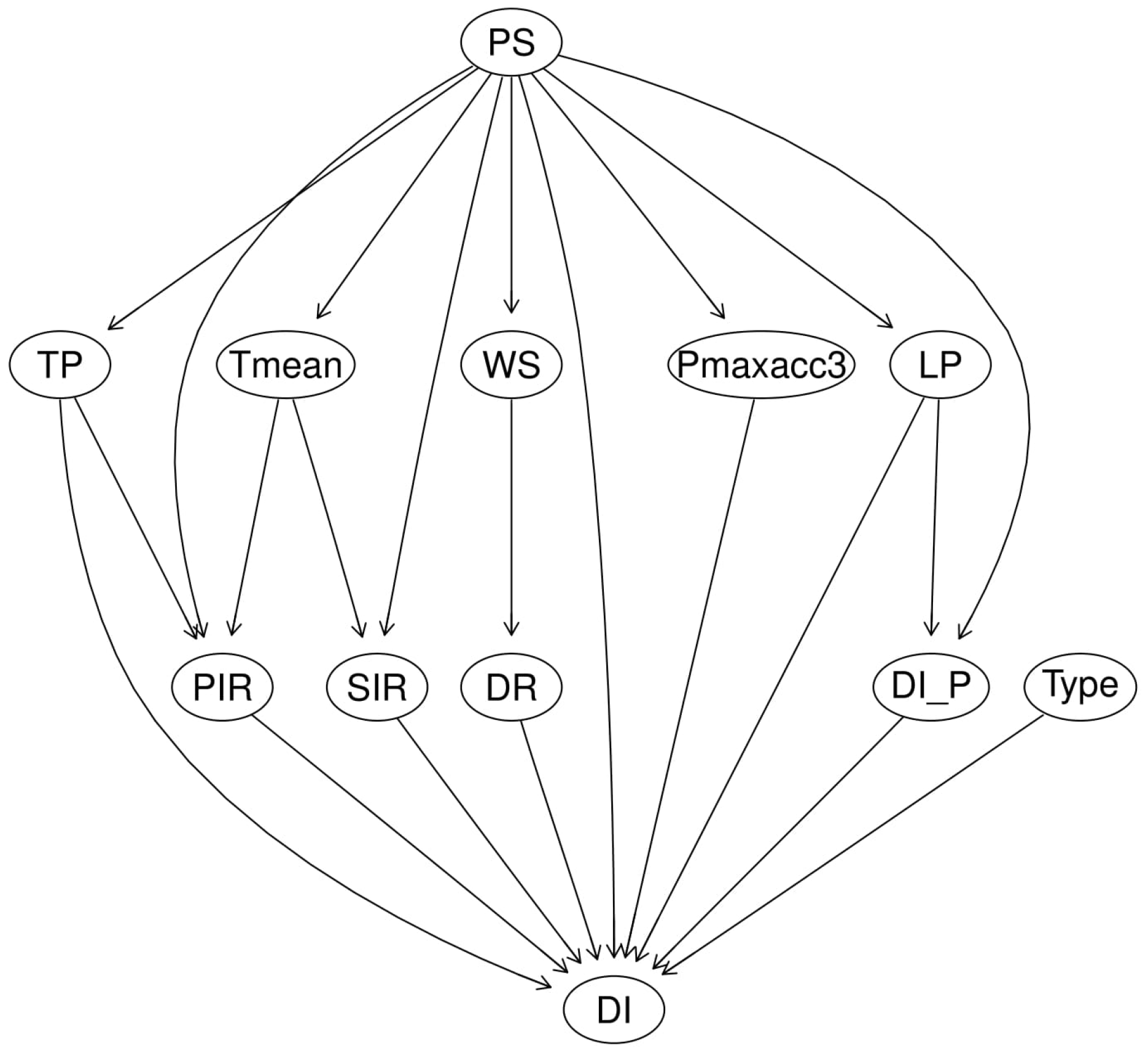
The representative DAG for the best-performing model under supervised (Case 2) and algorithm (Case 2) learning is shown in
Figure 6 and
Figure 7. In the case of supervised learning, the DAG is a plant stage based network. This network structure assumes: (1) the susceptibility of the grapevine to the PM development is influenced by changing weather and climate that varies by plant stage, (2) DI is independently affected by a set of factors including: precipitation (TP), primary infection rate (PIR), secondary infection rate (SIR), wind-speed (WS) influenced dispersal rate (DR), plant stage (PS), the degree-days based disease risk assessment model (
), latent period (LP), past DI (
); and genes cultivar types (Type). The network structure learned from supervised learning shows causal relationships based on existing knowledge, with dispersal rate (DR) of grape PM spores being influenced by wind-speed conditions, secondary infection (SIR), and temperature (
Figure 6). In algorithmic learning, causal relationships were generated from the independent random variables to maximum the network score of a network structure from bootstrap sampling technique with strength above 0.8 and direction above 0.5 from 5000 interactions. The learned model structure and linkages between variables from algorithmic learning (
Figure 7) shows DR not linked to DI as it was not identified as a significantly strong predictor. This suggests that DR needs to be better represented and that the current DR equation does not represent the observed PM epidemic. Significant correlations between grape cultivar types, plant stage (PS), and the risk assessment model (
) with DI was detected from the algorithmic learning.
The performance of the forecast model under supervised and algorithmic learning for the three northern grape cultivars for training (2000–2010), and prediction in 2011, is shown in
Figure 8. Both supervised and algorithm learning have similar model performance (both in MAE and RMSE). Model accuracy was high in the recorded drought years of 2000, 2002, and 2008 with values of MAE and RMSE were varying from 3 to 5 and from 4 to 7, respectively. The model performance worked well in non-drought years with MAE and RMSE were varying around from 0.56 to 2.6 and from 0.86 to 3.7, respectively. Model performance in both supervised and algorithm learning tended to be more and more accurate (smaller values in MAE and RMSE) in disease prediction in drought and non-drought years as the Bayesian network model has learned from more and more reliable input data. Disease performance in algorithm learning tends to be more sensitive in climate-related disease predictions than in supervised learning with MAE and RMSE in algorithm learning were higher than in supervised learning in drought years and smaller in non-drought years. The smallest value of MAE 0.99 and 0.56 in supervised and algorithm learning, respectively, found in 2011. The smallest value of RMSE 1.57 in supervised learning found in 2010 and 0.87 in algorithm learning found in 2011.
Model predictions of grape PM for the three cultivars from both supervised learning in Case 2 (dotted line) and algorithmic learning in Case 2 (dashed line) across the three plant stages of flowering, setting, and veraison are shown in
Figure 9. The predictions are shown compared to observed DI in 2011 (solid line). DI of conidial infection generally starts from the end of June until the end of the growing season. For Geisenheim-318 and Frontenac, the Bayesian network in both supervised and algorithm learning did work well in predicting disease incidence in 2011 with supervised learning has slightly better performance the hill-climbing-based algorithm learning in predicting DI over the growing season. Overall, the best model is Case 2 with supervised learning for which the model has learned using existing knowledge about disease development of grape PM using the full set of random variables but without relative humidity (as listed in
Table 2).
Forecast evaluation plots of DI in warm (dotted line) and cold (dashed line) years for the three cultivars: Chancellor (top), Geisenheim-318 (middle), and Frontenac (bottom) in 2011 by increasing and decreasing daily temperature in 2001 by
are shown in
Figure 10. The three grape cultivars have a similar response to the changing temperature but differ in the susceptibility to grape PM. In the warm year, DI tended to be higher than the normal for most of the growing seasons except in mid-August. The maximum DI over the growing season was higher in warm year than in the normal. while in the cold year, model prediction of DI has tended to lower than the normal except the beginning of August.
Evaluation of the optimal forecasting window for DI prediction of grape PM using the up to 16 days high-performance forecast data in GEFS is shown in
Figure 11. Averaged MAE and RMSE were calculated by taking the average of MAE and RMSE, separately, computed from the model predictions and actual disease incidence in different forecast windows. Lower values of MAE and RMSE indicate lower model uncertainty and higher model forecasting skill. The smallest values of averaged MAE were for 6 days forecasting (0.846), and the most significant values was for 16 days forecasting (0.926). Averaged MAE tended to decreased from 0.863 to the minimum values of 0.846 when forecasting windows changes from 1 to 6 days and increased to the maximum values of 0.926 when forecasting windows changes to 16 days. For averaged RSME, the smallest values were for one-day forecasting (1.029) and tended to the maximum values (1.344) when forecasting windows changed from 1 to 16 days. Overall, both averaged MAE and RMSE in up to 16 days forecasting windows were considerably small, our fungicide spray program was developed using the disease incidence predictions and climate variables from the GEFS in 16 days forecasting window.
We further compared our fungicide spray program to two existing benchmark programs, the UC-Davis, and the degree-days (with a
base temperature) based risk assessment model. The UC-Davis program is a score based program to provide suggestions for fungicide spray in different spray schedules. The UC score is a daily temperature-based model, which the model initials from the day of the first primary infection. The UC-Davis program applies fungicide spray with an interval of 14 to 21 days, if the UC score is less or equals to 30; a 10 to 17 days interval, if the UC score is from 40 to 50; or a 7-days interval, if the UC score is above 60. The degree-days based risk assessment model specified a spray schedule interval of 7 to 14 days, if
is above 1% in Chancellor and Geisenheim-318, and 0.5%, for Frontenac.
Figure 12 represents the application of the UC-Davis program and the degree-days based risk assessment model for disease control of grape PM at the experimental farm in Quebec in 2011. Fungicide spray applications from the UC-Davis exhibited a case of over-spraying in relation to the actual disease severity for each of the three cultivars. The UC scores were above 60 from 9 July until 18 September and suggests a high frequency of fungicide sprays. The degree-days based risk assessment model provided better disease control than the UC-Davis model by reducing the number of scheduled fungicide spray. This program suggested initial fungicide spray starts on 7 August for Chancellor, 10 August for Geisenheim-318, and 12 August for Frontenac.
The model-based fungicide spray program provides a spray strategy up to 6 days in advance and forecasts disease risk with a lead time of up to 10 days to optimize the efficiency of fungicide spray under the uncertainty of precipitation. An example of such a model-based fungicide spray program is for the date of 27 August, when a high rainfall event was forecast to occur on August 29 and 30 with precipitation of 46.46 mm and 121.129 mm, respectively (
Table 5). The table shows the average DI from 10 days of disease control under 6 different fungicide spray dates (28 August–2 September) for the three susceptible cultivars. The best spray day for the three grape cultivars was 1 September having an average DI of 22.72 for Chancellor, 9.47 for Geisenheim-318, and 3.82 for Frontenac.
Figure 13 shows 3D plots of 10-day daily DI for Chancellor (top-left), Geisenheim-318 (top-right), and Frontenac (bottom left) for the six different spray days, from a low to high level of disease severity. The 2D plot (bottom-right) shows the forecast daily DI for Chancellor (dotted line), Geisenheim-318 (dot-dashed line), and Frontenac (dashed line) on the optimal spray day.
7. Discussion
The best performing model for grape PM disease risk forecasting at the experimental farm in Quebec was Case 2 with model structure learned using supervised learning.
Figure 6 shows the learned structure found for this model. DI for the three cultivars was relatively consistent with the degree-days risk assessment model having a
base temperature and plant stage, but not with relative humidity included. Instead, the best local distribution of the causal relationship of DI involved total precipitation, primary infection rate, secondary infection rate, dispersal rate, plant stage, risk assessment model, latent period, and vary in susceptible cultivar type.
Figure 9 shows that the supervised Bayesian network has a very high performance in disease risk forecasting for the three susceptible cultivars over the plant stage that are affected by PM disease.
Model validation of DI shown in
Figure 9 shows the resultant model network structure from both supervised and algorithm learning. Supervised learning had a slightly better performance in predicting DI of grape PM over 2000–2011. Smaller values of MAE and RMSE in non-drought years than in drought years (i.e., 2000, 2002, 2008) indicates that the model has better forecasting skill in non-drought years, and the complex climate conditions significantly influence the development of DI in drought years, summarized in
Table 3. The development of PM in drought years was not well explained by the use of a simple binary factor suggesting that a more complex model of DI involving autocorrelation across multiple years (i.e., not just a single year factor) may be needed. The comparison result of the four selected model starting dates indicates the best time to initiate the modeling of disease incidence is when the disease occurs on the farm.
Model forecast evaluation results are shown in
Figure 10, whereby the three cultivars have a similar response to the changing temperature. There is a significant difference in DI between the normal year and the warm and cold years, which by adding or dropping the daily temperature by
, separately. DI tends to be more severe in warm years and less severe in cold years when compared to the DI in the normal year, which explains the complex interactions between the development of the pathogen of powdery mildew and its host under the influences of heat stress conditions. The warm temperature at the beginning of the growing season advances the bud break of the host as well as the development of ascospores from over-wintered cleistothecia. Then dispersal and infection, caused higher than normal DI.
The sensitivity analysis of model prediction of grape PM for the three cultivars in 2011 using the 16 days climate variable from GEFS shown in
Figure 11 indicates the GEFS data has very high performance in predicting DI in Quebec. Although the averaged MAE varied from 0.863 to 0.926 and averaged RMSE varied from 1.029 to 1.344 when forecasting window changes from day 1 to day 16, both averaged MAE and RMSE are all small (less than one percentage in averaged MAE and 1.5 percentage in averaged RMSE). The UC-Davis fungicide spray program shown in
Figure 12 shows an over-estimate of DI of PM of most of the growing season, results from over-spray suggestions of scheduled fungicide spray application in disease control.
The degree-days based risk assessment model provides better suggestions for disease control than the UC-Davis by delaying the initiation of the fungicide spray program for disease control. However, it does not consider the difference in susceptibility of cultivars. Our fungicide spray program was developed from the best-performing Bayesian network forecast model with supervised learning out to 16 days guided by GEFS reforecast climate. This program provides fungicide spray suggestions up to 6 spray day strategies with 10-days disease control forecasting by using information about forecast DI and the efficiency of fungicide spray under uncertainty climate changes (precipitations). An example of this is presented for 17 August 2011. This example data was selected because there are two significant forecast rainfall events on 29 August (46.46 mm) and 30 August (121.129 mm) and a few small rainfalls from 31 August–12 September.
Table 5 shows the best spray day for the three susceptible cultivars is on September 1st with results average DI of 22.72, 9.47, 3.82 for Chancellor, Geisenheim-318, and Frontenac, respectively, in 10 days after the spray has applied. The 3D plot in
Figure 13 shows model forecasts of DI extending out to 10 days in the future for the different spray days. The 2D plot shows the daily DI based on a current day for fungicide spray under variation to changing precipitation. With these forecast curves or foresight information output from the forecast model, grape producers can make a better decision about the best timing to apply fungicide spray for different grape cultivars in order to maximize the spray efficiency and to protect grapevines over the growing season.
8. Conclusions
Grape PM is one of the most common diseases responsible for significant reduction in grape yield in North America. The rate of development and epidemiology of this disease are influenced by regional-scale, longer-term climate and localized, shorter-term weather uncertainty. It also varies with growth stage and the genetics of a grape cultivar, making it difficult to develop efficient strategies for disease management. Most research on epidemiology and modeling of PM has been conducted for temperate climates. In this study, using 13 years of data, we developed and tested a novel Bayesian network model to forecast disease risk (i.e., the development of DI of conidial infection in grape PM on leaves) for three susceptible cultivars calibrated to site-specific data obtained from an experimental vineyard in Quebec. The forecast model generates high prediction (based on in-sample validation testing) also out to 16 days ahead using GEFS, and enables a reliable fungicide strategy for disease control with a 6-days forecasting window. Fully-independent validation data is needed to evaluate how well our model can forecast grape PM disease in other vineyards with differing grape cultivars, cultural practices, and environmental conditions.
There is observed uncertainty in DI that is not fully explained by our current model. Our modeling focuses on leaf PM epidemic and resistance at a time when the grape cluster is most susceptible to the presence of PM, whereby leaf infection is usually the first warning and signal to the vines treatment and leaf protection is a limiting factor to grape yield. Nonetheless, relying solely on leaf resistance is a current shortcoming of the forecast model. An operational protection model would need to consider leaves and grape berry clusters. This would require extending the current model to be spatially-explicit, because berry clusters are sufficiently complex in terms of their development and exhibit susceptibility that is spatially heterogeneous within vineyards and strongly dependent on phenological age [
27]. Recent spatial model simulations of fungicide use show that applying a fungicide early at flowering may significantly reduce PM diseased area, by up to 81% at the end of the season by delaying the epidemic onset. It also helps to maintain a low level of disease and to minimize potential PM dispersion from leaves to bunches [
43]. Burie et al. (2011) demonstrate the strong dependence of PM disease progression on grapevine growth rate (vigor) and regional climate using a multi-scale dynamic grapevine-PM model [
44]. Future work stemming from the current study will require spatio-temporal vineyard data and additional data from other measurement variables such as: canopy leaf wetness, fungicide type, and efficiency, spatial locations of susceptible grape cultivars, and berries infection, yield loss.
The developed model-based fungicide spray program provides an improved way to minimize the total number of sprays and their timing for optimizing grape PM spray efficiency and its recommendations could, in the future, be used by vineyard producers through the growing season, as the total proportion of the infections of over-wintered ascospore is a critical factor in determining the outbreak of conidia over an entire season. Nonetheless, skillful protection of grapevines by contact, translaminar, or systemic fungicides also helps to address unexplained uncertainty and current shortcomings of the model-based forecasts.

 ,
, 


