Abstract
In this work, simple tuning rules for feedforward compensators were applied to design a control strategy to regulate the inside air temperature of a greenhouse during daytime by means of a natural ventilation system. The developed control strategy is based on a PI (Proportional-Integral) controller combined with feedforward compensators to improve the performance against measurable external disturbances such as outside air temperature, solar radiation, and wind velocity. Since the greenhouse process dynamics is very complex and physical non-linear models are mathematically complicated, a system identification methodology was proposed to obtain simpler models (high-order polynomial and low-order transfer functions). Thus, an easier procedure was completed to tune the PI controller parameters and to obtain the feedforward compensators expressions by following a series of modern and simple tuning rules. Simulations with real data were executed to compare the control performance of a PI controller with or without the addition of feedforward compensators. Moreover, real tests for the developed control strategy were carried out in an experimental greenhouse. Results demonstrate an enhanced control performance with the presence of the feedforward compensators under different weather conditions.
1. Introduction
Climate control for greenhouses is critical for optimal crop production. Since a greenhouse is a closed environment, climate regulation can ensure an appropriate growth of the crop. The air temperature inside the greenhouse considerably affects to the physiological processes of the plants and, thus, it is important to regulate it in an adequate range depending on the crop variety and the geographical location of the greenhouse. This accelerates its growth and increases the production quality while economizing energy consumption [1].
Controlling the greenhouse climate requires different types of systems to cause a particular effect on the inside climatic variables. The predominant systems are ventilation and heating, but advanced greenhouses can use modern systems such as carbon dioxide injection or artificial lights. Even so, automatic control applied to greenhouses is a complicated problem. The external weather conditions should be considered as disturbances in the formulation of the control problem since they constantly cause undesirable changes in the inside climatic variables.
Focusing on automatic control for the inside air temperature of a greenhouse, previous works have been published in the literature in which different control techniques were tested or simulated. Some references to diverse works for air temperature control by means of natural ventilation are cited here: PID (Proportional-Integral-Derivative) control [2,3,4,5], adaptative control (multirate) [6,7,8], multivariable and nonlinear Model Predictive Control (MPC) [9,10,11], optimal control [12], robust Quantitative Feedback Theory (QFT) control [13,14], neural network control [15,16], event-based control [17,18], hybrid control [19], and fuzzy logic control [20,21].
In comparison with the prior cited studies, in this work, a simple but effective control solution focused on disturbances rejection was pursued to regulate the greenhouse air temperature using natural ventilation. Feedforward (FF) control is a basic strategy to reduce the effect of measurable disturbances on the process output and it is commonly implemented in combination with a PID controller in order to improve the performance of the feedback loop. In Reference [22], a non-linear FF control strategy was calculated and evaluated in simulation based on a non-linear greenhouse model. In contrast, in this manuscript, a different and simpler approach is proposed to calculate linear FF compensators. The main contribution of this work is the use of simple modelling and control approaches that can be easily implemented in any real greenhouse. First, system identification methods are applied to obtain reduced linear models of the greenhouse micro-climate dynamics. Then, the resulting models are used to design the FF compensators by utilizing the innovate tuning rules proposed in Reference [23]. These tuning rules are based on linear models of the process and are focused on improving the control system performance by minimizing the Integral Absolute Error (IAE). Notice that it is the first time that these tuning rules are experimentally tested.
The document is organized as follows—in Section 2 materials and methods are described, where a detailed explanation of the experimental greenhouse, system identification methods and developed control strategies can be found. Section 3 is dedicated to discuss the most relevant results concerning the identified models, simulation results, comparison of different control schemes, and the real FF control tests performed in the experimental greenhouse. Finally, in Section 4, some conclusions and future works are mentioned.
2. Materials and Methods
2.1. Experimental Greenhouse
Control tests for this work were performed in an experimental greenhouse (Figure 1) situated at the Cajamar Foundation Experimental Centre “Las Palmerillas” (Almería, Spain). This traditional “parral-type” greenhouse has a surface of 877 m2 (37.80 m × 23.20 m) and it is equipped with modern actuators to control the micro-climate under the cover. Some examples of the available actuators are humidification and dehumidification systems, pipe heating system, carbon dioxide enrichment system and natural ventilation system.
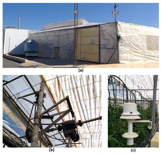
Figure 1.
Experimental greenhouse: (a) Exterior view in which roof and side vents can be observed. (b) Motor for the roof vents. (c) Inside air temperature and humidity sensor protected with a solar radiation shield.
In this work, the developed control strategies are focused on utilizing the natural ventilation system. This system consists of five zenithal windows (8.36 m × 0.73 m) placed at the roof of the cover and two lateral windows (32.75 m × 1.90 m) positioned along the north and the south sides of the greenhouse. Three AC motors (0.37 kW and 2 × 0.18 kW) are utilized to automate the vents opening depending on the desired opening percentage (from 0% to 100%) calculated by the climate controllers. The desired opening percentage is achieved by sending an electrical current to each motor during a specific time interval.
Several climate monitoring systems are distributed inside the greenhouse in order to precisely obtain measurements from a large amount of sensors. In addition, a weather station is installed outside the greenhouse to register external climate variables. In particular, a probe (HC2S3, Campbell Scientific Ltd., Shepshed, UK) is used to measure the air temperature inside and outside the greenhouse. For the external solar radiation, a pyranometer (LP02, Hukseflux, Delft, The Netherlands) is employed, and measurements of the external wind velocity are provided by an anemometer (A100L2, Vector Instruments, Rhyl, UK). These sensors are connected to a series of acquisition devices (Compact FieldPoints, National Instruments, Austin, TX, USA) and the measurements are transmitted by an Ethernet network to a supervisory control and data acquisition (SCADA) system. Experimental data for this work were obtained from the mentioned monitoring systems with a sampling period of 30 s for each climatic variable.
2.2. System Identification Methodology
The micro-climate inside a greenhouse is a highly complex process that involves multiple variables, phenomena, time scales and non-linear dynamics. According to referent studies in the literature [1], this micro-climate can be modelled by a set of differential equations expressing energy transfers and mass balances. These type of complex models, based on first principles, are usually obtained to accurately simulate the dynamics of the process. However, these complex models are difficult to be mathematically managed in order to calculate control strategies. For this reason, system identification methods were utilized in this work to obtain black-box simplified models for the dynamics of the process occurring in a greenhouse.
System identification techniques allows to represent complex systems by using linear models based on data collected from input-output experiments performed in the real process. In the discussed case of a greenhouse, the inside micro-climate variables are strongly affected by the outside environmental conditions (disturbances) and the state of the actuators. For this work, the inside air temperature of the greenhouse was the desirable variable to be controlled by only using the natural ventilation system. Therefore, a simple model was required to capture the effect of the main disturbances and the natural ventilation on the inside air temperature. Notice that low-order models are required to design the control approach. However, due to the complexity of the greenhouse dynamics, first, a high-order linear model is obtained to capture the process behaviour, and afterwards, the model is reduced to a low-order model for control purposes.
As a previous step, some tests were carried out in the experimental greenhouse to register data from various days for the system identification procedure. In each test, the natural ventilation system was programmed to offer a changing signal with different ventilation opening percentages during the day. Hence, the effect of the natural ventilation on the inside air temperature could be properly reproduced by the model to be identified.
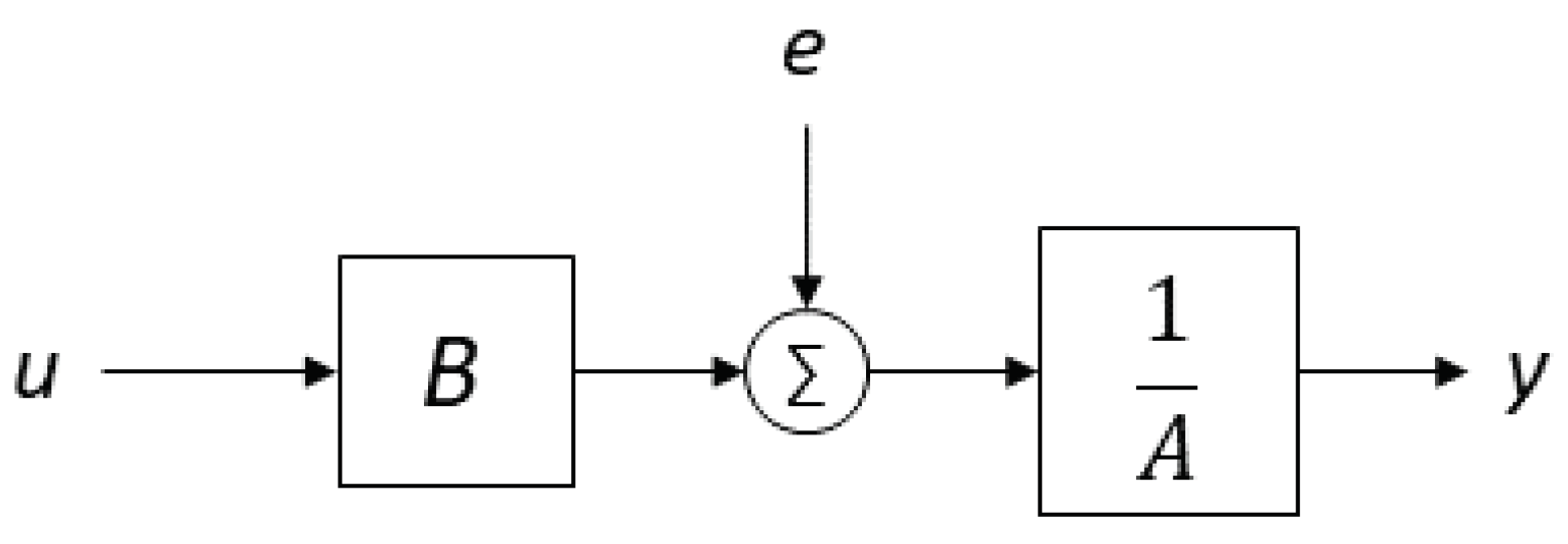
In the automatic control field, one of the most used structures are the autoregressive models [24], which coefficients can be easily determined through an identification procedure. For this work, an auto-regressive with exogenous input (ARX) model was selected to obtain the high-order empirical model for the inside air temperature of the greenhouse. A simple graphical description for an ARX model is shown in Figure 2 for a Single-Input and Single-Output (SISO) system.
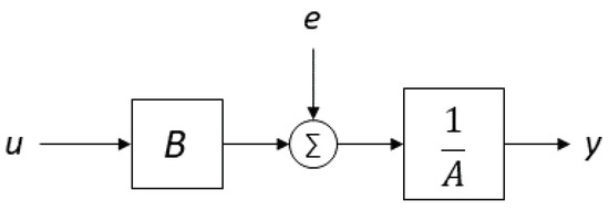
Figure 2.
Simple graphical representation for an auto-regressive with exogenous input (ARX) model.
In particular, the implemented ARX model for this work is a Multiple-Input and Single-Output (MISO) model (see Section 3.1) that can be mathematically represented in discrete-time form by the following expression:
where y is the output, are the inputs, e is the white noise, is the total number of inputs and is the number of samples corresponding to each input time delay. and are polynomials with the following structure:
where and are the order for polynomial A and B, respectively, and a and b are the coefficients to be determined in the identification procedure with real data of the process.
Once the high-order ARX model was obtained, a model reduction stage was accomplished for control purposes as commented above. In this model reduction stage, the relationship for each input with the output was modelled as a first-order model described by a transfer function expressed in Laplace domain for continuous time as follows [25]:
where is the static gain, is the time constant and is the time delay (dead time), all referred to the ith input. Thanks to transfer function models, the development of automatic control strategies can be easily achieved as explained in the following Section 2.3.
2.3. Automatic Control Strategies
The control problem faced in this work consists in keeping the diurnal inside air temperature (controlled variable) close to a desired reference value (setpoint) by regulating the opening of the windows (manipulated variable) of the natural ventilation. The natural ventilation system is based on the air exchange occurring between the interior and the exterior of the greenhouse. The inside air temperature of the greenhouse is generally higher than the outside air temperature (due to the greenhouse effect). Every time that the vents are opened, the cooler and more dense outdoor air enters the greenhouse causing the hotter and less dense inside air to rise and exit through the roof vents. However, the following difficulties should be taken into account in order to design an appropriate control strategy [1]:
- The greenhouse micro-climate is strongly affected by disturbances, both measurable and non-measurable. Thus, the designed controller should consider the effect of the outside weather conditions.
- The motors of the natural ventilation system present two limitations: (i) actuator saturation, due to a limited opening range from 0% to 100%; and (ii) resolution, since the windows opening is performed in steps of 10%.
These issues have been considered in the proposed control approach as described in the following sections.
2.3.1. PID Control
The Proportional-Integral-Derivative (PID) controller is the most extended feedback control technique in most industrial processes and it is the one selected for this work because of its simplicity and high flexibility [25]. The PID controller allows to calculate a control action depending on the existing error between the measured process output and the desired setpoint. A basic PID controller can be mathematically expressed as follows:
where u is the control signal and e is the control error. The main parameters of a PID controller are the proportional gain, , the integral time, , and the derivative time, . The values for these parameters can be calculated based on different tuning methods depending on the desired control response and the process dynamics [25]. A common formulation for a PID controller as a transfer function in Laplace domain is presented in Equation (6) and a basic feedback control scheme based on a PID controller is shown in Figure 3.

Figure 3.
Block diagram of a simple feedback loop with a Proportional-Integral-Derivative (PID) controller, , applied to a process represented with a transfer function, .
In this work, a PI (Proportional-Integral) controller was selected and the derivative term was omitted mainly because of the noisy signals in the real facilities. An additional modification was made to the basic structure of a PI controller in order to take into account the saturation of the ventilation motors. An anti-windup mechanism based on the back-calculation technique was incorporated to the PI controller to prevent the undesirable “windup” effect of the integral term [25]. When the actuator is saturated, the anti-windup mechanism shown in Figure 4 is designed to reset the integrator value to zero by adding the signal multiplied by the tacking constant . The parameter is an adjustable term to regulate how rapidly the integrator is reset.
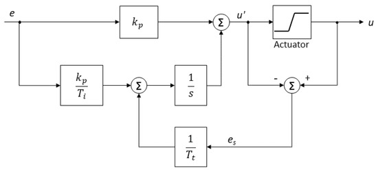
Figure 4.
Block diagram of a PI (Proportional-Integral) controller with an anti-windup mechanism.
The lambda () method was selected as the tuning approach to calculate the parameters for the PI controller and to impose a desired behaviour for the feedback control response. According to this method, the PI controller parameters are calculated using the following expressions [25,26]:
where is the desired time constant for the closed-loop response, and k, and L are the parameters of the first-order model used to describe the process behaviour.
2.3.2. Feedforward Control
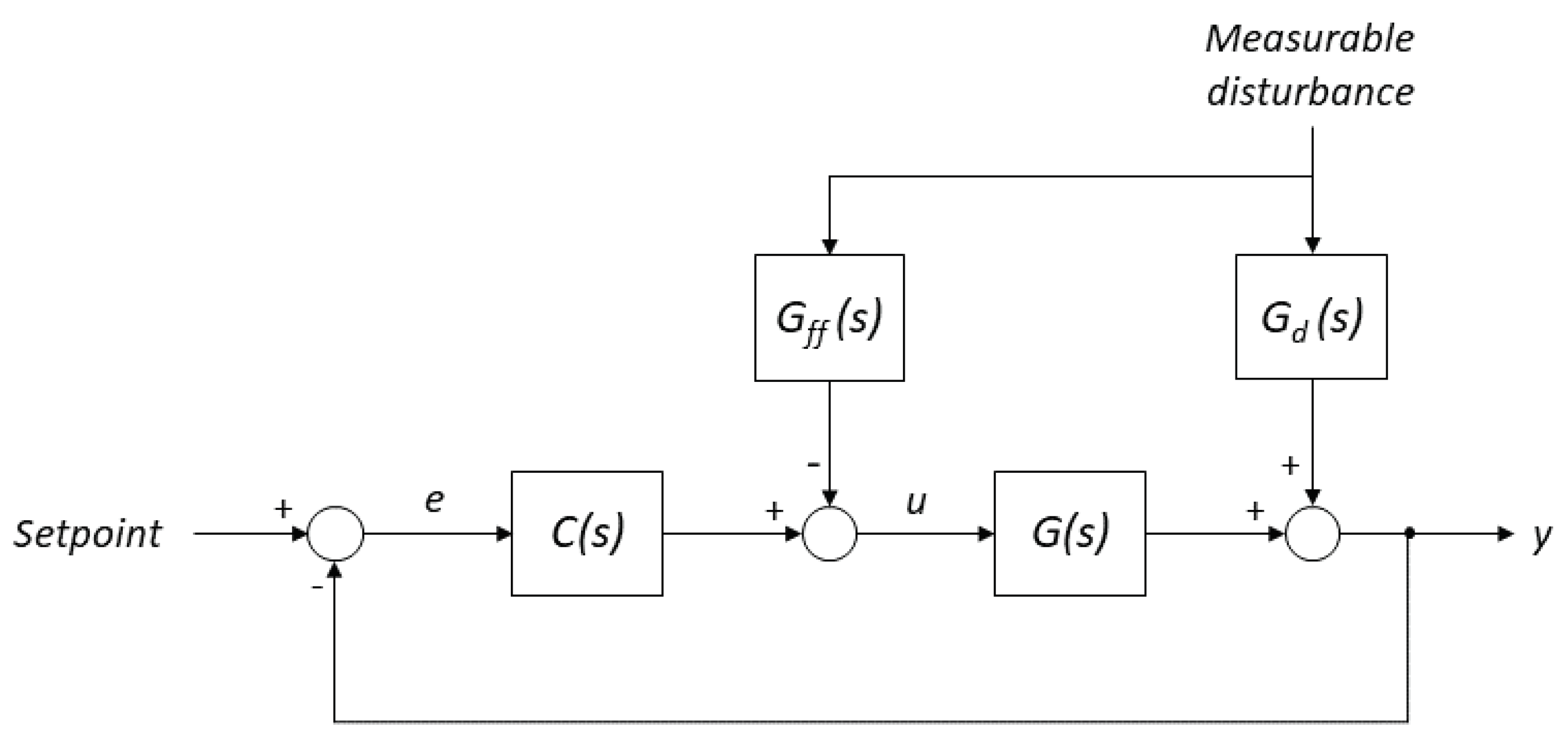
A classical feedforward control approach has been selected in this work to account for the measurable disturbance rejection problem. The basic control scheme is shown in Figure 5. The idea consists in adding a new block called feedforward compensator, , that tries to reduce the effect of the disturbances before they affect to the process output [27].
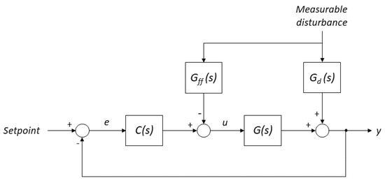
Figure 5.
Simple feedforward control scheme, where is the feedback controller, is the process transfer function, is the feedforward compensator, and is the transfer function modelling the effect of the measurable disturbance on the output of the process.
The classical way to calculate the feedforward compensator is given by the following expression:
where is the process model describing the dynamics between the process output, y, and the control signal, u; and is the model that describes the dynamics between the process output and the disturbance signal, d.
As observed from Equation (9), the perfect realization of the feedforward compenstator is only feasible when there is no causality issues. Typically, there exist inversion problems because of the time delay of is smaller than in G. So, when perfect compensation is not possible, it is common in practice to omit the non-realizable part and to implement the rest of the compensator, or just to implement a static feedforward by using only the static gains of and G. These solutions allow to implement the feedforward control block and to eliminate the disturbance effect in steady-state, but the process output performance is considerably deteriorated.
Recently, this issue about feedforward compensator design has been analyzed in the literature, where simple tuning rules to account for the inversion problems have been proposed [23,28,29]. In this work, the tuning rules proposed in Reference [23] have been used. The tuning rules take into account the parameters of the process model as well as the action of the feedback controller during the design stage of the FF compensator. As a result, a guideline summary is proposed in order to minimize the IAE of the control approach while obtaining a disturbance rejection without overshoot.
The tuning rules are based on the assumptions that G and are described by first-order-plus-dead-time (FOPDT) models and the feedforward compensator is a lead-lag filter as follows:
Then, the feedforward compensator is calculated according to the following guideline:
- Set:
- Calculate as:
- Calculate the compensator gain, , considering the PI controller parameters ( and ):
Results for the design of the FF compensators with the mentioned simple rules are presented and discussed in Section 3.3 and Section 3.4.
2.4. Software
MATLAB® (MathWorks, MA, USA) and Simulink® were used to develop and simulate the different control strategies presented in this work. Specifically, the System Identification Toolbox™ was used to obtain the ARX model and the low-order models expressed as transfer functions. Additionally, the PI controller and the feedforward compensators were programmed in MATLAB® code in discrete-time form and embedded in a SCADA system for real tests in the experimental greenhouse.
3. Results
3.1. ARX Model
The developed ARX model intended as a MISO model is shown in Figure 6. For the system identification procedure, no distinction was made among the model inputs with the purpose of obtaining a simple prediction model. However, the outside weather variables should be considered as measurable disturbances. The three main disturbances affecting the inside air temperature were selected based on previous studies [1]: external solar radiation, external air temperature and external wind velocity.

Figure 6.
Representative diagram for the implemented ARX model.
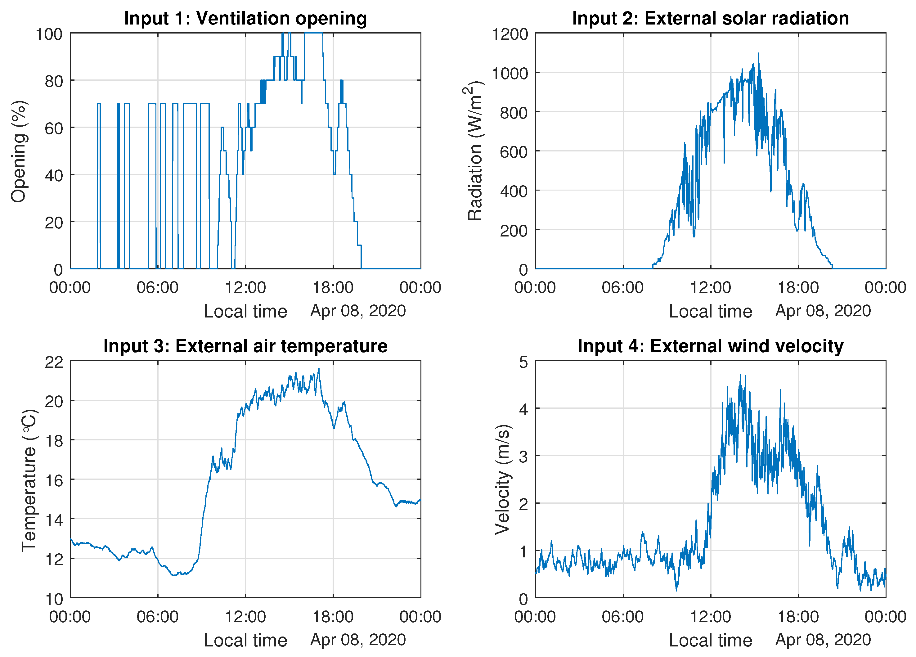
The ARX model was obtained with the system identification procedure explained in Section 2.2. A series of different ventilation tests were performed in the experimental greenhouse during spring 2020 in order to record a sufficient dataset for a proper model identification. In each test, diverse operational conditions were registered focusing on different ventilation opening profiles so that the data could represent the variety of the real greenhouse dynamics. Figure 7 shows an example for the inputs of the ARX model identification. The ventilation opening graphics reveals two different behaviours. During the night, the vents are usually closed and only some periodical openings are required if an active control for inside air humidity is being performed (depending on the crop necessities). During daytime, the ventilation opening varies depending mainly on the imposed limits for the inside air temperature control. Due to the weather conditions of the south-eastern of Spain and the dimensions of the experimental greenhouse, the vents are normally fully opened when the maximum level for external solar radiation occurs. The selected data for identification present a typical range of variation for climatic variables during the spring period at the location of the greenhouse.
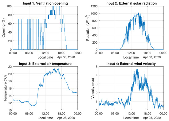
Figure 7.
Inputs for ARX model identification.
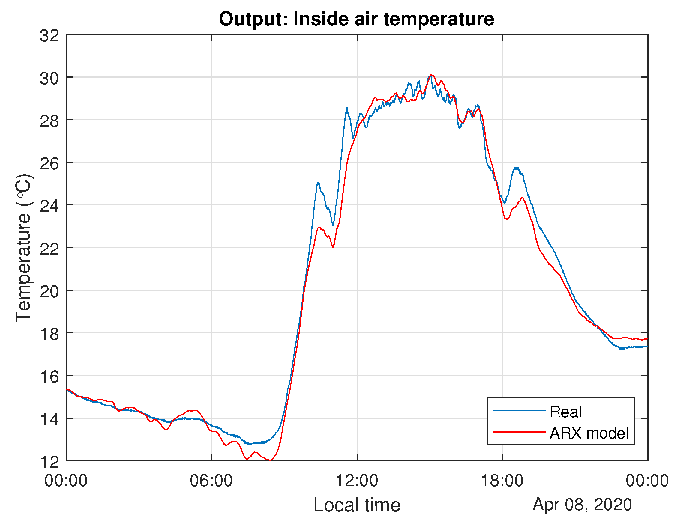
So, the stored input data was used with the System Identification Toolbox™ in MATLAB® and several ARX models were obtained, selecting the one with best goodness of fitting. Figure 8 shows an example of the validation results for one day. As observed, the resulting linear model captures the main dynamics of the real inside air temperature. An statistical evaluation of the error between the real temperature and the predicted temperature by the model was accomplished. The mean absolute error for the model is 0.49 °C, the standard deviation is 0.63 °C, and the maximum absolute error is 2.82 °C. These values for the error are comparable to the ones obtained in previous studies [1]. Furthermore, simulations with data from other days offered a similar response for the ARX model. Hence, it can be concluded that the ARX model is validated to predict the inside air temperature of the greenhouse for control purposes.
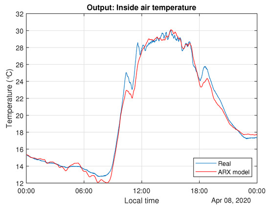
Figure 8.
Results for ARX model identification compared against real inside air temperature.
The identified ARX model is a high-order model (10th-order) and its corresponding set of polynomials are presented in Equations (17)–(21).
Despite the fact that the calculated ARX model is a high-order model, the validity of these types of models is constrained to particular conditions, which means that the model is effective for prediction when the input data are similar in operational conditions to the data that were used for model identification. In consequence, different ARX models should be identified to be utilized on different seasons of a year or during a crop cycle. Nevertheless, as shown in this work, an ARX model can be a simple and a reasonably reliable tool to obtain low-order models for the input-output relationships of a complex dynamic model, mainly with the intention of designing automatic control strategies.
3.2. Low-Order Models
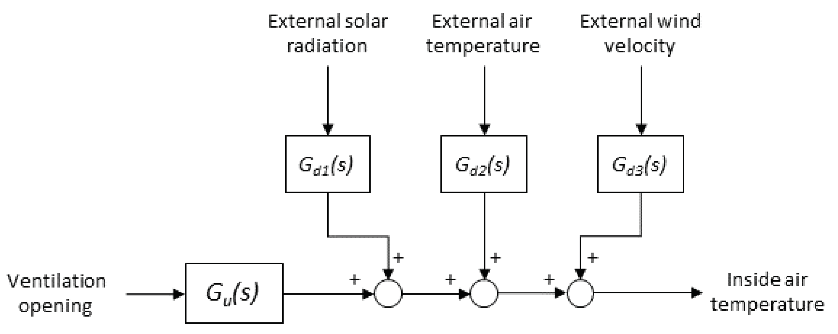
Now, the high-order ARX model described in the previous section is reduced to low-order models to facilitate the control design stage. As a result, four different low-order models will be obtained such as shown in Figure 9. On the one hand, the relationship between the natural ventilation and the inside air temperature of the greenhouse is given by the process transfer function, . On the other hand, three additional transfer functions, , are obtained for each of the disturbances.
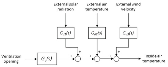
Figure 9.
Transfer function models for input-output and disturbance-output relationships.
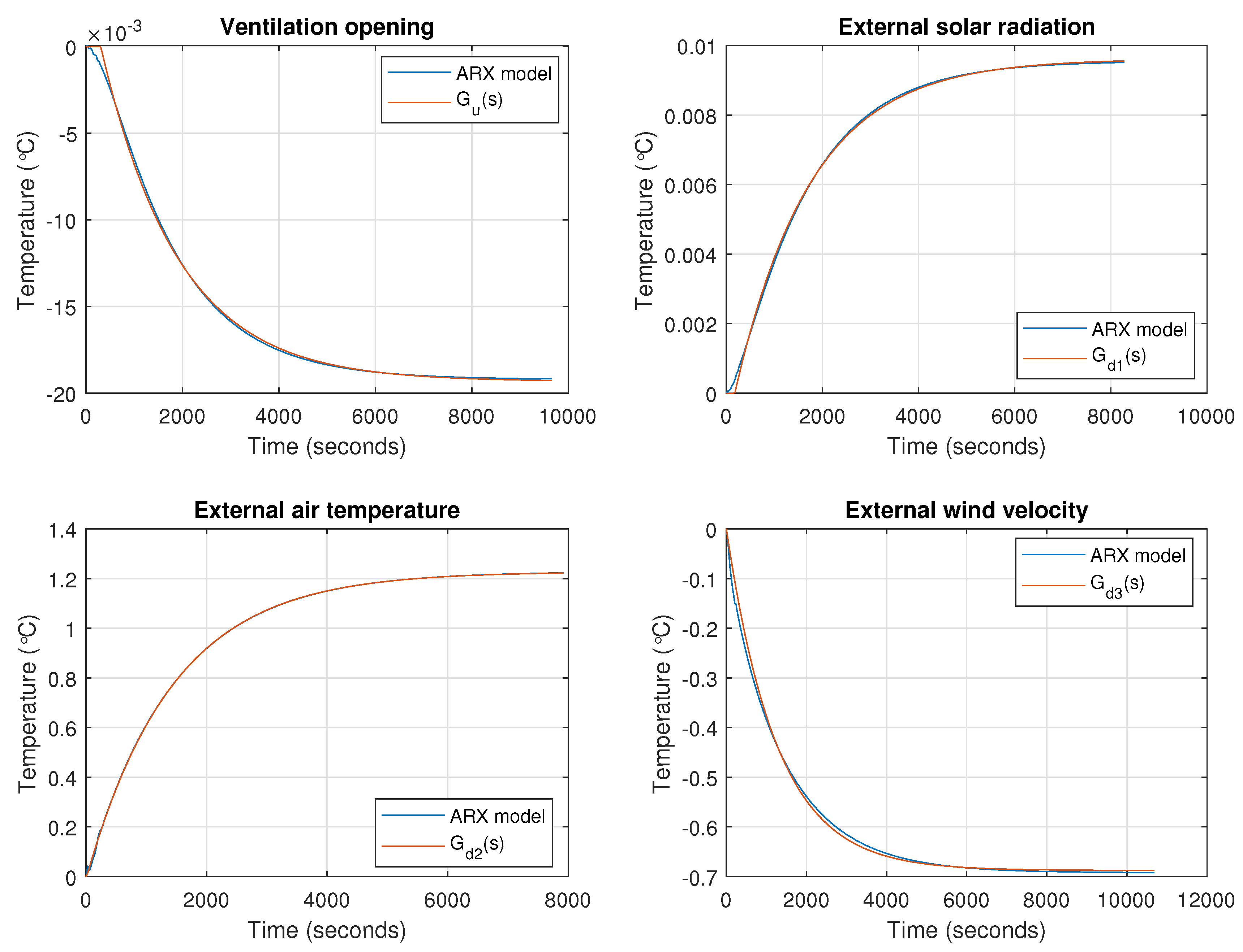
The procedure to reduce the high-order ARX model consists in utilizing an unit step signal as input for the ventilation opening while the disturbances are set to zero. Then, the transient response for the inside air temperature predicted by the ARX model is analyzed applying the reaction curve method to calculate the characteristic parameters of a transfer function. The same actions are applicable to find a model for a measurable disturbance, in this case, the unit step signal is for one of the disturbances while setting to zero the ventilation opening and the remaining disturbances. The structure for the transfer functions was imposed as a first-order model with or without dead time, depending on the different transient responses. This procedure was smoothly accomplished with the System Identification Toolbox™ in MATLAB®. In Figure 10, a graphical comparison is presented to confirm that the transfer function models accurately capture the dynamics predicted by the ARX model.
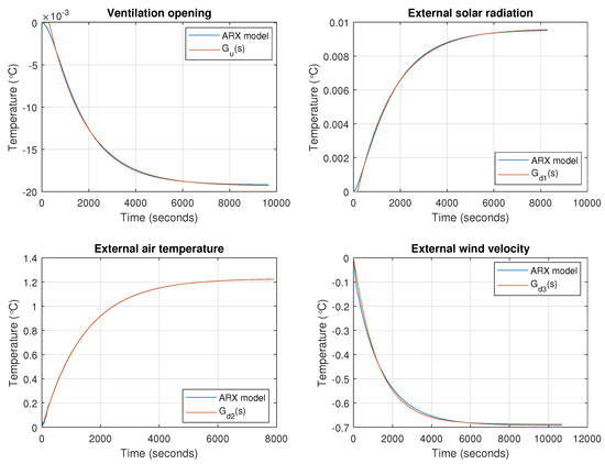
Figure 10.
Unit step responses of the ARX model (for each input) compared against the transient responses of the transfer function models.
The identified first-order transfer functions are formulated in Equations (22)–(25), where the values of the parameters are rounded whereas a higher precision was preserved for MATLAB® calculations. These models are then utilized in the next section to design the PI controller and to calculate the FF compensators following the methods described in Section 2.3.
3.3. Design and Simulation of Control Strategies
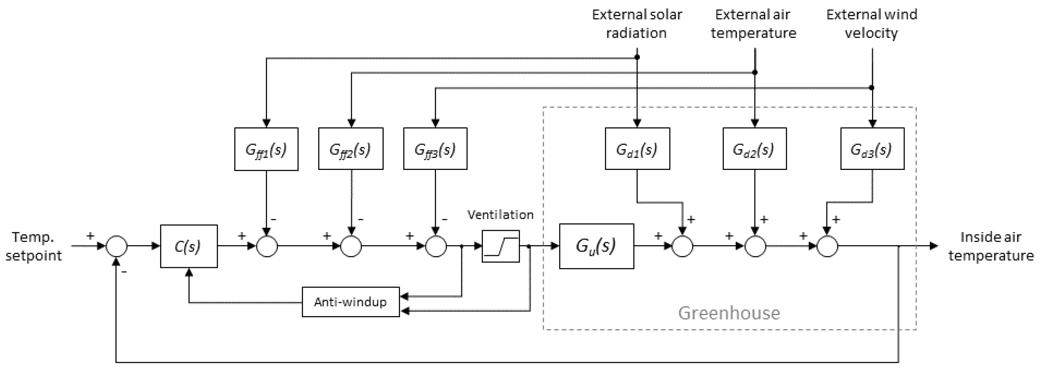
The proposed control strategy in this work is a combination of a PI controller with feedforward compensators. The implementation scheme can be observed in Figure 11. This control scheme tackles the problem of temperature control for a greenhouse in a simple way, but taking into account the particularities mentioned in Section 2.3 regarding the presence of disturbances and the limitations of the actuators for natural ventilation.
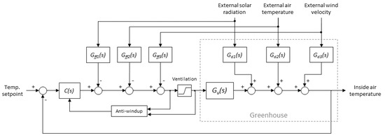
Figure 11.
Control scheme for the inside air temperature of a greenhouse.
The PI controller was calculated by applying the lambda tuning method and considering the parameters of the process transfer function obtained in Equation (22). A time constant for the closed-loop of 0.3 times the open-loop time constant () was imposed to offer a rapid response against unmeasurable disturbances and possible changes for the setpoint value. According to Equations (7) and (8), the resulting parameters for the PI controller are and . Additionally, for the anti-windup mechanism, the coefficient (see Figure 4) was established as [25].
Once the PI controller was tuned, the FF compensators were calculated. A summary for the designed FF transfer functions is presented in Table 1. Firstly, classical FF compensators, , were determined with Equation (9). As can be observed, perfect realization was not possible since a causality problem appears due to the dead time of the process transfer function (see Equation (22)), which is greater than the dead times of the disturbances transfer functions. Thus, the time delay terms were excluded. When the simple tuning rules from Equations (13)–(15) were applied to determine the FF compensators, the same problem occurs with the time delays satisfying . However, the main advantage of these innovative rules is that the time delays can be taken into account to calculate the pole and the gain of the FF first-order transfer functions (if proven ). Hence, slight differences in values for the parameters of the modern FF compensators compared against the classical approach can be observed in Table 1.

Table 1.
Feedforward compensators comparison.
Simulations were executed in Simulink® to evaluate the performance of the control scheme before testing it in the experimental greenhouse. A Simulink® model was built to reproduce the structure shown in Figure 11, in which the ARX model was utilized as the predictor for the inside air temperature of the greenhouse. The sample time for the Simulink® model execution was fixed in 30 s, the same as in the real control system. Additionally, the limitation of the vents motors was taken into account with a saturation block and a function to imitate the real resolution by approximating the control signal to step intervals of 10%.
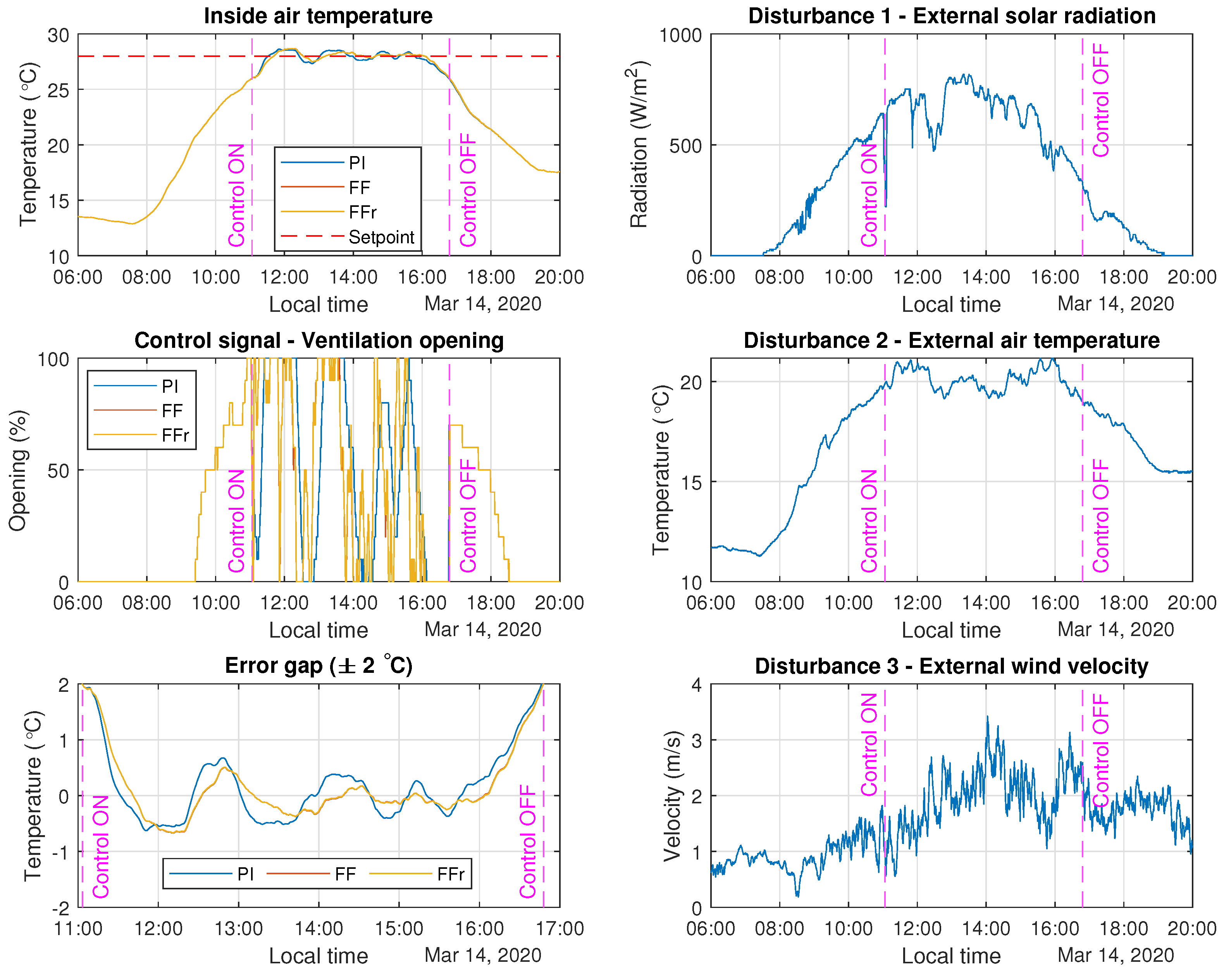
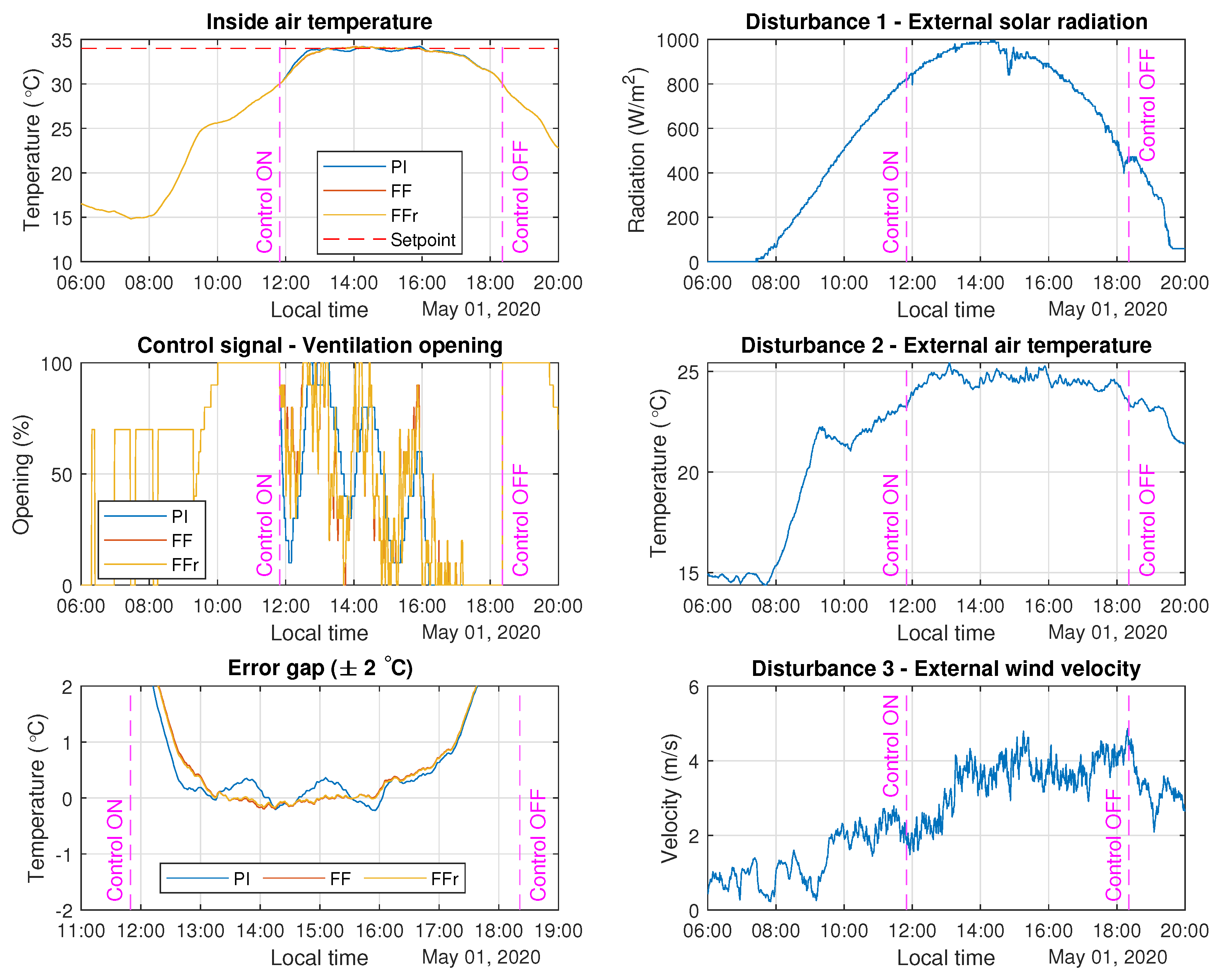
For each simulation test, three variations of the control scheme were individually executed with data from the same day in order to compare the graphical differences between the following control strategies—(i) PI control, (ii) PI control plus classical FF compensators, and (iii) PI control plus FF compensators calculated with the simple tuning rules. The results for the simulation with data from 14 March 2020 are shown in Figure 12. In each graph, the time gap when the automatic control is active is indicated by two dashed vertical lines. The graph for the inside air temperature shows an acceptable control response closed to the desired temperature setpoint. Analyzing the graph for the error signal, it is clearly noticeable that, as expected, the PI controller without FF compensators presents an oscillatory response when rejecting the disturbances. When the FF compensators are included, the control response is smoother and the controlled variable is maintained closer to the setpoint. In regard to the control signals, saturation occurs for the PI controller during a longer time, but its control signal is less aggressive compare to the FF control. Nevertheless, the control signal for the FF control was expected to be more varying since the values of the three disturbances have to be cancelled in each time instant.
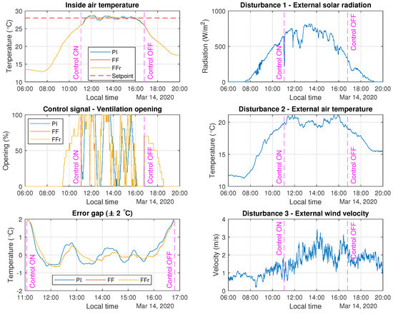
Figure 12.
Results for simulation with data from 14 March 2020.
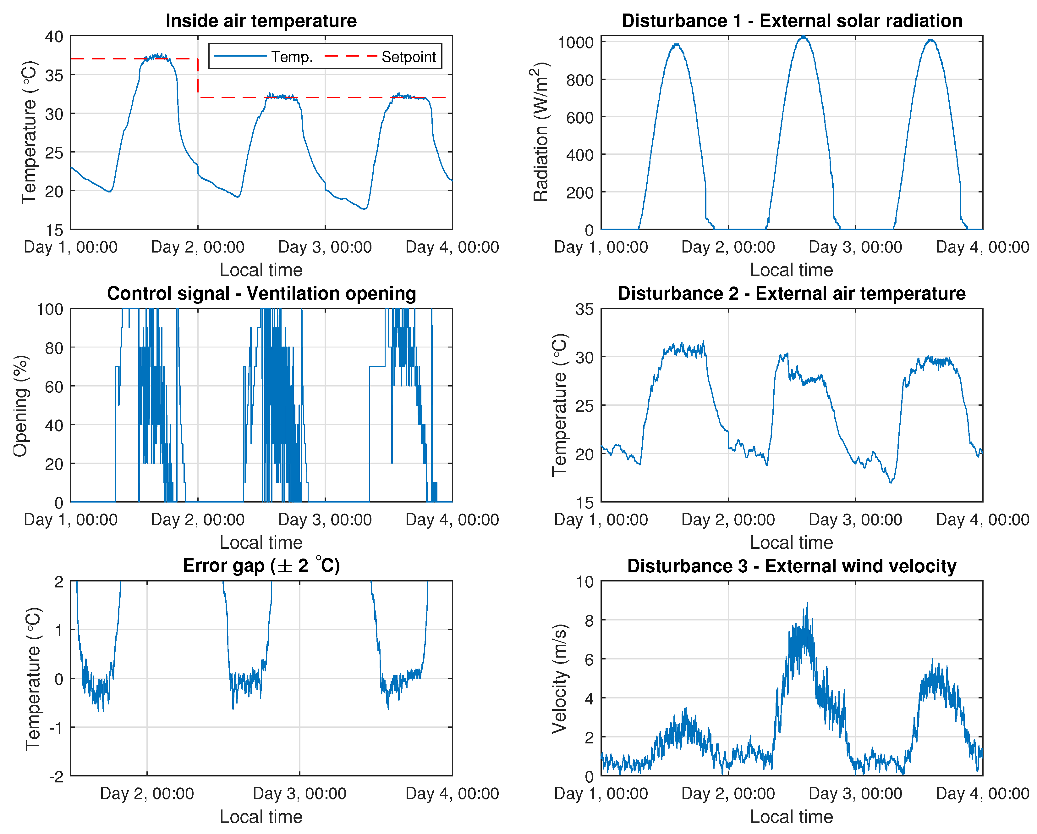
A different simulation was executed with data from 1 May 2020 and the results are presented in Figure 13. In this case, a higher value for the setpoint was established in order to test the control behaviour at a different operational point. Also, the presence of significant changes on external disturbances is reduced compared to the previous simulation. In the graph for the inside air temperature, it can be concluded the effectiveness of the control strategies, considering that the controlled variable is practically regulated at the imposed setpoint. In the error gap graphic, it is confirmed that the FF control is superior to the PI control, presenting an undisturbed response. Finally, in this case, the control signal for FF control is less aggressive since the changes in the disturbances occur with smaller magnitude.

Figure 13.
Results for simulation with data from 1 May 2020.
In Table 2, the IAE values are presented for each control strategy in order to offer a quantitative comparison for the previous simulation results. The IAE values were calculated from the first time instant when the process output reached the setpoint until the last time instant when the output distanced from the setpoint. In both days, the IAE is significantly lower for the FF control strategies compared to the PI control, as expected. Regarding the FF control strategies, the best performance is achieved by the simple tuning rules for FF compensators, presenting the lowest values for IAE in both simulations. The IAE minimization was one of the objectives of applying the simple tuning rules for FF control. Although the IAE differences compared to the classical FF compensators may seem not important for a single day, the accumulated IAE when considering a full crop season would be relevant.

Table 2.
Integral Absolute Error (IAE) comparison.
As observed in the results for the simulations, in order to control the inside air temperature during daytime, a reachable setpoint should be fixed for the midday hours. If the automatic control is activated at dawn, a lower setpoint would be established. As the sun rises during the diurnal period, the external solar radiation and the external air temperature cause an increase in the inside air temperature. Thus, the setpoint would be rapidly surpassed and the actuators would be saturated to maintain the vents with an opening of 100%. This problem can be solved by activating the automatic control at a desired time instant by means of a bumpless control transfer mechanism [25]. When the midday hours are reached, this mechanism will allow to switch to the automatic controller if the process was being manually controlled until that time instant, for example. The bumpless control transfer mechanism was enabled in Simulink® for the PI controller and it was also implemented in code for the real tests in the greenhouse, as explained in the following Section 3.4.
3.4. Real Tests with Feedforward Control
For the control tests in the experimental greenhouse, only the FF compensators calculated with the simple tuning rules were evaluated, being the first time ever that these rules are tested in a real process. The control scheme from Figure 11 was adapted to a discrete-time script coded in MATLAB® to be on-line executed in the SCADA system of the greenhouse. The sample time of the control loop corresponds to 30 s.
For each control test, a procedure was followed to activate the control algorithm only during the midday hours. Initially, another climate controller for the greenhouse was active and the natural ventilation was regulated mainly to maintain the inside air humidity in an optimal range for the crop. When the inside air temperature approximates the midday hours and the solar radiation is close to its maximum value, the previously described bumpless control transfer mechanism allowed to switch the automatic control to the PI controller and the FF compensators implemented for this work.
Three tests were executed on different days in the greenhouse. The tests were performed on the last weeks of spring, when the most unfavorable weather conditions for greenhouses in Almería appear, so it was an excellent opportunity to evaluate the developed control strategy under hostile daytime temperatures. These tests were not carried out on continuous days, but the results are combined and presented in Figure 14 for a better visualization. Before analyzing the results, it is important to highlight that the FF compensators were tested in a different manner on each day to analyze better their effects. On the first day, FF compensators for external solar radiation and external air temperature were active, excluding the compensator for external wind velocity. On the second day, all the FF compensators were utilized. Finally, on the third day, only the compensator for external air temperature was active.
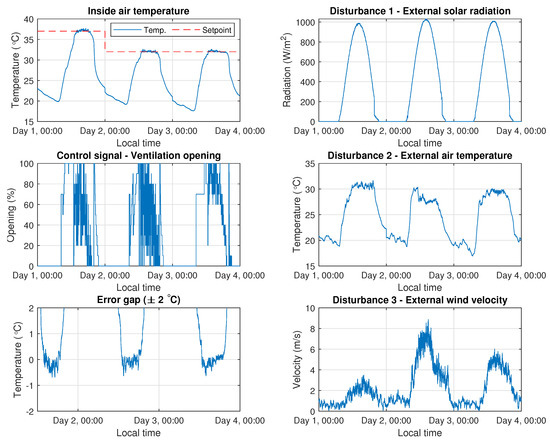
Figure 14.
Real control tests performed at the experimental greenhouse.
As can be observed in Figure 14, a satisfactory response is obtained for the inside air temperature, which is controlled at different setpoints. In the error gap graphic, the presented errors are contained in an interval smaller than ±1 °C. Therefore, it can be confirmed the remarkable performance of the control strategy considering the limitations of the ventilation motors and all the simplifications that were carried out to obtain the parameters for the PI controller and the FF compensators.
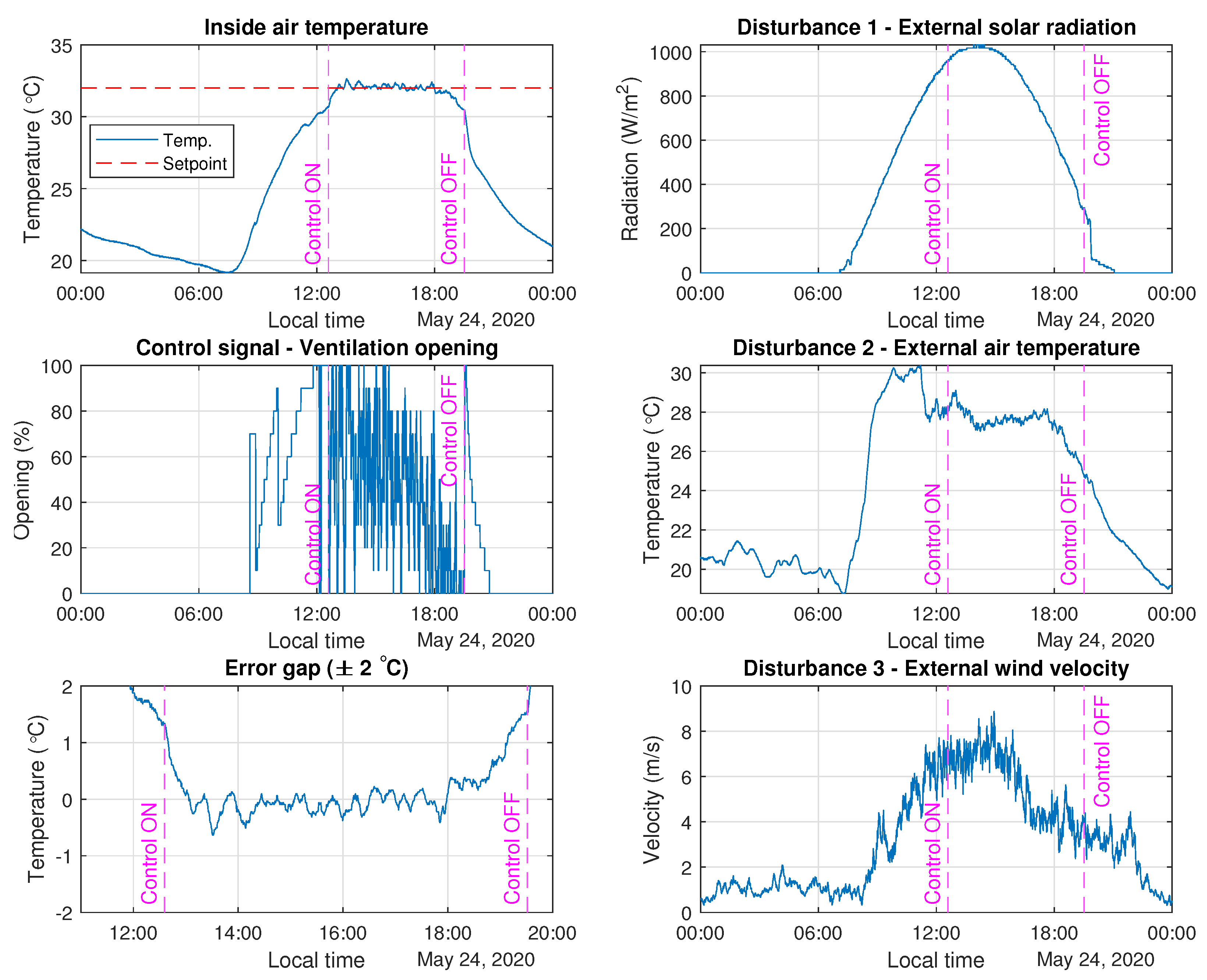
Figure 15 shows the best control results corresponding to day 2 in detail. The inside air temperature is correctly controlled at the desired setpoint, with no significant deviations. In this day, all the FF compensators were active and, thus, the control signal for the ventilation opening is visibly varying. All the disturbances seem to be well rejected by the FF compensators on this windy day with an external air temperature that was not as stable as compared to day 1 and 3.
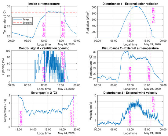
Figure 15.
Real control test from 24 May 2020. All the feedforward compensators were active.
On day 2, the automatic control was activated at 12:35 by means of the previously described bumpless control transfer mechanism. During the first minutes, the control strategy determined that it was necessary to close the vents to reach the setpoint for the inside air temperature. Since the external solar radiation was still rising and the external air temperature presented a peak at 13:00, the FF compensators caused the ventilation to open progressively before the inside air temperature had reached the setpoint. Thanks to this change in the control signal, the inside air temperature did not increase excessively. Once the solar noon happened at 14:10, the control error remained near to zero, since the temperature inside the greenhouse was stabilized at the setpoint. However, in order to regulate the temperature near to the setpoint, the FF compensators had to deal with external air temperature variations and specially with the external wind velocity, which presented several rapid changes. For this reason, the control signal is significantly varying, and some transitions from 100% to 0% of ventilation opening occurred in time intervals of 15 min. As the external solar radiation decreases, only intermediate values (between 20% and 60%) were necessary for the ventilation opening. This tendency for the control signal was logical to avoid the decrease of the inside air temperature until the automatic control was disabled at 19:30.
4. Conclusions
In this paper, a control strategy based on simple tuning rules for feedforward compensators was designed and tested in a real greenhouse to control the inside air temperature by means of a natural ventilation system. The main objective of this work was to propose a simple but effective control scheme for a complex non-linear process, such as the micro-climate inside a greenhouse. The feedback controller was designed as a PI controller, which parameters were calculated by the lambda tuning method. The limitations of the ventilation actuators were taken into account with an anti-windup mechanism. For the FF control, the classical approach was compared to a series of novel tuning rules proposed in Reference [23]. These simple tuning rules have been tested in a real process for the first time in the present work.
A system identification methodology was accomplished to obtain a high-order ARX model. The main advantage of using an ARX model to simulate the dynamics of the greenhouse climate was the simplicity of the procedure to identify the model, since only a data-set of particular climatic variables was required. However, a remarkable disadvantage is the need to recalculate a new ARX model for different seasons of the year, due to the strong dependence of the greenhouse micro-climate on the meteorological variations of its location. The high-order ARX model was then reduced to low-order models expressed as first-order transfer functions. The transfer functions offered simplified models to easily calculate the PI controller parameters and the FF compensators. Some simulations were executed and the benefits of including FF compensators for disturbances rejection were evidenced when compare to PI control without FF compensation.
The designed control strategy presented positive results for the real tests performed in the experimental greenhouse. The inside air temperature was effectively controlled at different setpoints, under diverse operational conditions, and control errors were contained in an interval smaller than ±1 °C. Although disturbances rejection was satisfactory considering the limitations of the ventilation actuators, some slight imperfections appeared in the real tests due to the modeling simplifications and other non-measurable disturbances affecting the inside air temperature.
Future works may be focused on identifying more models for different seasons of the year, in order to design controllers and FF compensators for a wide range of operational conditions. Furthermore, additional FF compensators for important measurable disturbances, such as the inside soil surface temperature, could be included to improve the performance of the proposed control strategy.
Author Contributions
A.P.M.-R. was the responsible of the work, the design of the control approach and the writing of the manuscript. F.G.-M. was the responsible of the experimental results and the implementation issues. J.L.G. contributed to the elaboration of the manuscript and revision, and the control process design. F.R. was the responsible of the discussion section and the revision of the manuscript. All authors have read and agreed to the published version of the manuscript.
Funding
This work has been funded by the National R+D+i Plan Project DPI2017-85007-R of the Spanish Ministry of Science, Innovation and Universities and ERDF funds.
Acknowledgments
Author Francisco García-Mañas is supported by an FPU grant of the Spanish Ministry of Science, Innovation and Universities. Authors also want to express their gratitude to the Cajamar Foundation Experimental Center.
Conflicts of Interest
The authors declare no conflict of interest.
Abbreviations
The following abbreviations are used in this manuscript:
| ARX | Auto-Regressive with eXogenous input |
| FF | FeedForward |
| FOPDT | First-Order-Plus-Dead-Time |
| IAE | Integral Absolute Error |
| MISO | Multiple-Input and Single-Output |
| MPC | Model Predictive Control |
| PI | Proportional-Integral |
| PID | Proportional-Integral-Derivative |
| QFT | Quantitative Feedback Theory |
| SCADA | Supervisory Control And Data Acquisition |
| SISO | Single-Input and Single-Output |
References
- Rodríguez, F.; Berenguel, M.; Guzmán, J.L.; Ramírez-Arias, A. Modeling and Control of Greenhouse Crop Growth; Springer: Berlin/Heidelberg, Germany, 2015. [Google Scholar]
- Davis, P. A technique of adaptive control of the temperature in a greenhouse using ventilator adjustments. J. Agric. Eng. Res. 1984, 29, 241–248. [Google Scholar] [CrossRef]
- Cunha, J.B.; Couto, C.; Ruano, A. Real-time parameter estimation of dynamic temperature models for greenhouse environmental control. Control Eng. Pract. 1997, 5, 1473–1481. [Google Scholar] [CrossRef]
- Setiawan, A.; Albright, L.D.; Phelan, R.M. Simulation of greenhouse air temperature control using PI and PDF algorithms. IFAC Proc. Vol. 1998, 31, 111–117. [Google Scholar] [CrossRef]
- Hu, H.; Xu, L.; Wei, R.; Zhu, B. Multi-objective control optimization for greenhouse environment using evolutionary algorithms. Sensors 2011, 11, 5792–5807. [Google Scholar] [CrossRef] [PubMed]
- Arvanitis, K.; Paraskevopoulos, P.; Vernardos, A. Multirate adaptive temperature control of greenhouses. Comput. Electron. Agric. 2000, 26, 303–320. [Google Scholar] [CrossRef]
- Berenguel, M.; Yebra, L.; Rodríguez, F. Adaptive control strategies for greenhouse temperature control. In Proceedings of the 2003 European Control Conference (ECC), Cambridge, UK, 1–4 September 2003; pp. 2747–2752. [Google Scholar]
- Rodríguez, F.; Guzmán, J.; Berenguel, M.; Arahal, M. Adaptive hierarchical control of greenhouse crop production. Int. J. Adapt. Control. Signal Process. 2008, 22, 180–197. [Google Scholar] [CrossRef]
- Senent, J.S.; Martinez, M.A.; Blasco, X.; Sanchis, J. MIMO predictive control of temperature and humidity inside a greenhouse using simulated annealing (SA) as optimizer of a multicriteria index. In Proceedings of the International Conference on Industrial, Engineering and Other Applications of Applied Intelligent Systems, Castellón, Spain, 1–4 June 1998; Springer: Berlin/Heidelberg, Germany, 1998; pp. 271–279. [Google Scholar]
- Blasco, X.; Martínez, M.; Herrero, J.M.; Ramos, C.; Sanchis, J. Model-based predictive control of greenhouse climate for reducing energy and water consumption. Comput. Electron. Agric. 2007, 55, 49–70. [Google Scholar] [CrossRef]
- Gruber, J.; Guzmán, J.; Rodríguez, F.; Bordons, C.; Berenguel, M.; Sánchez, J. Nonlinear MPC based on a Volterra series model for greenhouse temperature control using natural ventilation. Control Eng. Pract. 2011, 19, 354–366. [Google Scholar] [CrossRef]
- Ioslovich, I.; Gutman, P.O.; Seginer, I. A non-linear optimal greenhouse control problem with heating and ventilation. Optim. Control. Appl. Methods 1996, 17, 157–169. [Google Scholar] [CrossRef]
- Linker, R.; Gutman, P.; Seginer, I. Robust controllers for simultaneous control of temperature and CO2 concentration in greenhouses. Control Eng. Pract. 1999, 7, 851–862. [Google Scholar] [CrossRef]
- Hoyo, A.; Moreno, J.C.; Guzman, J.L.; Rodríguez, F. Robust QFT-Based Feedback Linearization Controller of the Greenhouse Diurnal Temperature Using Natural Ventilation. IEEE Access 2019, 7, 64148–64161. [Google Scholar] [CrossRef]
- Fourati, F.; Chtourou, M. A greenhouse control with feed-forward and recurrent neural networks. Simul. Model. Pract. Theory 2007, 15, 1016–1028. [Google Scholar] [CrossRef]
- Qu, Y.; Ning, D.; Lai, Z.; Cheng, Q.; Mu, L. Neural networks based on PID control for greenhouse temperature. Trans. Chin. Soc. Agric. Eng. 2011, 27, 307–311. [Google Scholar]
- Pawlowski, A.; Guzman, J.L.; Rodríguez, F.; Berenguel, M.; Sánchez, J.; Dormido, S. Simulation of greenhouse climate monitoring and control with wireless sensor network and event-based control. Sensors 2009, 9, 232–252. [Google Scholar] [CrossRef]
- Pawlowski, A.; Guzmán, J.; Normey-Rico, J.; Berenguel, M. Improving feedforward disturbance compensation capabilities in Generalized Predictive Control. J. Process Control 2012, 22, 527–539. [Google Scholar] [CrossRef]
- Rajaoarisoa, L.H.; M’Sirdi, N.K.; Balmat, J.F. A case study of a hybrid controller design of a class of hybrid system application to a greenhouse micro-climate control. In Proceedings of the CCCA12, Marseilles, France, 6–8 December 2012; pp. 1–6. [Google Scholar]
- Lafont, F.; Balmat, J.F. Optimized fuzzy control of a greenhouse. Fuzzy Sets Syst. 2002, 128, 47–59. [Google Scholar] [CrossRef]
- Riahi, J.; Vergura, S.; Mezghani, D.; Mami, A. Intelligent Control of the Microclimate of an Agricultural Greenhouse Powered by a Supporting PV System. Appl. Sci. 2020, 10, 1350. [Google Scholar] [CrossRef]
- Rodríguez, F.; Berenguel, M.; Arahal, M. Feedforward controllers for greenhouse climate control based on physical models. In Proceedings of the 2001 European Control Conference (ECC), Porto, Portugal, 4–7 September 2001; pp. 2158–2163. [Google Scholar]
- Guzmán, J.L.; Hägglund, T. Simple tuning rules for feedforward compensators. J. Process Control 2011, 21, 92–102. [Google Scholar] [CrossRef]
- Ljung, L. System Identification: Theory for the User, 2nd ed.; Prentice Hall PTR: Upper Saddle River, NJ, USA, 1999. [Google Scholar]
- Åström, K.J.; Hägglund, T.; Astrom, K.J. Advanced PID Control; ISA—The Instrumentation, Systems, and Automation Society: Research Triangle Park, NC, USA, 2006; Volume 461. [Google Scholar]
- Dahlin, E. Designing and tuning digital controllers. Instrum. Control Syst. 1968, 41, 77–83. [Google Scholar]
- Guzmán, J.L.; Hägglund, T.; Veronesi, M.; Visioli, A. Performance indices for feedforward control. J. Process Control 2015, 26, 26–34. [Google Scholar]
- Rodríguez, C.; Guzmán, J.L.; Berenguel, M.; Hägglund, T. Generalized feedforward tuning rules for non-realizable delay inversion. J. Process Control 2013, 23, 1241–1250. [Google Scholar] [CrossRef]
- Veronesi, M.; Guzmán, J.L.; Visioli, A.; Hägglund, T. Closed-loop tuning rules for feedforward compensator gains. IFAC-PapersOnLine 2017, 50, 7523–7528. [Google Scholar] [CrossRef]
© 2020 by the authors. Licensee MDPI, Basel, Switzerland. This article is an open access article distributed under the terms and conditions of the Creative Commons Attribution (CC BY) license (http://creativecommons.org/licenses/by/4.0/).


