Abstract
The principles of sustainable agriculture in the 21st century are based on the preservation of basic natural resources and environmental protection, which is achieved through a multidisciplinary approach in obtaining solutions and applying information technologies. Prediction models of bioavailability of trace elements (TEs) represent the basis for the development of machine learning and artificial intelligence in digital agriculture. Since the bioavailability of TEs is influenced by the physicochemical properties of the soil, which are characteristic of the soil type, in order to obtain more reliable prediction models in this study, the testing set from the previous study was grouped based on the soil type. The aim of this study was to examine the possibility of improvement in the prediction of bioavailability of TEs by using a different strategy of model development. After the training set was grouped based on the criteria for the new model development, the developed basic models were compared to the basic models from the previous study. The second step was to develop models based on the soil type (for the eight most common soil types in the Republic of Serbia—RS) and to compare their reliability to the basic models. From the total number of developed models by soil type (80), 75% were accepted as statistically reliable for predicting the bioavailability of TEs by soil type and 70% of prediction models had a higher determination coefficient (R2), compared to the basic models. For the Fluvisol soil type, all prediction models were accepted, while the least reliable prediction was for the Planosol type. As in the previous study of bioavailability prediction for TEs, the prediction models for Cu stood out, with more than half of the models with R2 greater than 0.90. Results of this study indicated that the formation of a testing set by soil type derives models whose predictions are more reliable than the basic ones. To improve the performance of prediction models, it is necessary to include additional physicochemical parameters and to conduct an adequate analysis of extensive testing sets with more comprehensive statistical techniques.
1. Introduction
Natural resources of trace elements (TEs) in the environment consist of stone and soil [1], where the soil has the main role in the control of their bio-presence [2]. International legislation, as well as the guidelines for soil quality, are usually based on the total concentration of the trace elements [3,4,5], apart from in individual countries such as the Netherlands [6], Belgium, Slovakia [7], the United Kingdom [8] and the Republic of Serbia [9], in whose regulations it is stated that the maximum amount of TEs in the soil are modified in relation to specific soil parameters (pH levels, soil organic matter (SOM), clay and texture class). The general opinion is that the contemporary approach to evaluating the quality of soil and the level of risk to human health based on the total amount of TEs is inadequate and insufficient [10,11]. This opinion is justified by the fact that only the soluble and mobile fraction of TEs can enter the food chain through adsorption by plants [12]. TEs in soil must be mobile before they can become bioavailable to plants and other soil biota [13]. Bioavailable concentrations of heavy metals in soil are significantly lower in comparison to the total concentrations and depend on the soil properties and the heavy metal [12,13,14,15,16].
Bioavailability of TEs has a double effect on cultivated plant species, negative in case of the uptake of non-essential and essential TEs in concentrations that are phytotoxic, and desirable in the case of the intake of required amounts of essential TEs [17]. These facts indicate that modeling of TEs’ bioavailability can be used in assessing the risk of contaminated soil exploitation, as well as in assessing the excess or deficit of essential TEs [18]. Based on bioavailability, it is possible to conduct a risk assessment, and predict the transport, fate and potential environmental impact of TEs [19]. Thus, the information obtained by applying prediction models for the bioavailability of TEs is an important tool that can be used in good agricultural practice and environmental protection.
The burdens on environmental science and engineering regarding cost, workforce, space requirements and time consumption could potentially be reduced by prediction models [20]. The synergy of agricultural practice, science and computer technologies through machine learning and artificial intelligence (AI) forms highly predictive mathematical models that are based on patterns and structures hidden in large and high-dimensional data sets [21]. One of the statistical techniques used in the formation of prediction models for machine learning and AI is multiple linear regression [20,21,22,23,24]. Freundlich’s model is obtained by applying multiple linear regression, which makes it one of the potential models that can be used for artificial intelligence and machine learning. Models formed based on the Freundlich equation (or Freundlich models) were used to predict the sorption of TEs in soil [23,24,25,26,27,28,29], the bioavailability of TEs [30,31,32,33,34,35], and the bioaccumulation of TEs in plants [12,36,37,38,39,40].
Predictive factors that influence the above mentioned processes in the soil and the soil-plant system, such as the numerous physical and chemical properties of the soil and the mechanisms of the adoption of TEs by the plants, are used to form the training set. The physical and chemical properties include the content of clay fraction, organic matter (total SOM and/or water-soluble DOM), cation exchange capacity (CEC), total DTPA, EDTA, soluble and water-soluble forms of TEs, iron/manganese/aluminum oxide, pH, texture class, liquid–solid ratio for TEs and chemical speciation TEs [13,18,23,24,36,41,42,43,44], and have been used in prediction models by many authors [18,40,45,46,47,48,49,50,51,52,53,54,55,56,57]. The most commonly used quantitative prediction variables are pH, SOM and total content of TEs [36,58]. The model development in our previous study [31] included pH, clay, organic matter, and pseudo-total forms of TEs extracted by aqua regia (TEAR) as parameters for predicting the content of bioavailable forms of TEs:
log (TEDTPA) = A + b*pH + c*log(SOM) + d*log(Clay) + e*log(TEAR).
A study by Dinić et al. [31] concluded that, in order to obtain more reliable prediction models, it is desirable to divide the tested dataset based on the chemical and physical parameters of soil (pH values, types of SOM, carbonate content) or by the type and manner of soil use, which is consistent with research by other authors [18,53,54,55,59,60]. The bioavailability of TEs is also influenced by the type of soil [2,10], and since the physicochemical properties are specific to each soil type due to the pronounced pedogenetic diversity, it is necessary to predict the bioavailability of TEs individually for each soil type.
The type and composition of soil significantly affect the retention of TEs, which is more pronounced in soils with a higher proportion of fine particles. This property is associated with the high reactivity of fine particles that contain minerals of clay, iron/manganese/aluminum oxide and humic acid [61]. The sorption strength of TEs is characteristic of soil type [62], since the processes of sorption and bioavailability of TEs are influenced by soil mineral composition, iron/manganese/aluminum oxide and hydroxides, silicates, phosphates, carbonates, soil and humic acids, and organic colloids [44,61,63]. Depending on the mentioned physicochemical properties and processes in the soil, the mobility of TEs can vary greatly in different soil types [15,64].
The aim of this study was to examine the influence of soil type on the reliability of the prediction model for the bioavailability of TEs. The initial hypothesis is that the separation into subgroups of the tested data set by soil type will provide more reliable prediction models for individual trace elements, via the selection of soil predictive parameters with the greatest impact on the bioavailability of TEs for each soil type. To confirm the initial hypothesis, a tested set of data from our previous study [31] was used to form a model for the most common soil types in the territory of RS.
2. Material and Methods
According to its geographical location and natural characteristics, the Republic of Serbia (RS) is a Central European, Balkan, Pannonian and Danubian country [65]. The soil cover of RS is not large in area but is significant for the variety of its systematic units, which arose as a result of the diversity of conditions of origin and development of the soil [66]. Of the total area of the RS, agricultural soil occupies 65.2% [67]. The most common soil types by area occupied in relation to the total number of soil types in RS are Chernozem (17.68%), Cambisol (27.99%), Fluvisol (7.57%), Gleysol (6.25%), Regosol (2.18%), Planosol 5.54%), Arenosol (0.72%) and Vertisol (8.32%) [65].
Samples of disturbed soil were collected from agricultural soil of the Republic of Serbia in the period 2010–2018. Each composite sample consisted of 20–25 individual samples, which were sampled by a gouge auger from a 30 cm depth. Sampling locations covered by model 1 were the Municipality of Veliko Gradište, Mačva and Toplica districts and sections of the E75 Highway through RS from Belgrade to Preševo, while for the model 2, locations from sections of the E75 Highway through RS from Belgrade to Preševo were excluded from the total sample number (Figure 1). The total area covered by this research was 6345 km2, of which 54.8% was agricultural soil (obtained from the Corine Land Cover data set) [68]. Preparation of samples and physicochemical analysis of the soil were conducted and comprehensively described in the previous study [31].
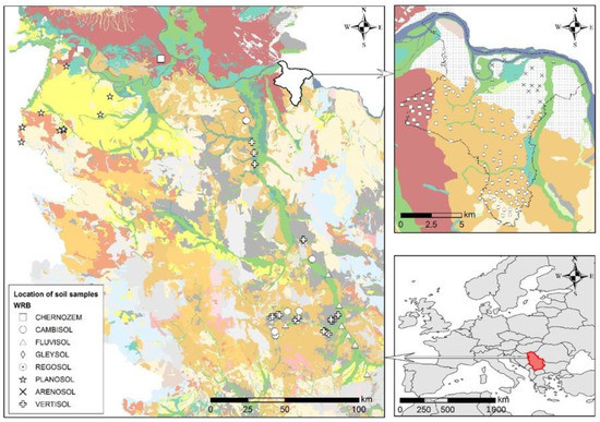
Figure 1.
Soil sampling locations with soil type in the Republic of Serbia.
2.1. Statistical Analysis
For the purposes of this research and the development of prediction models by soil type, a total of 240 samples from our previous study [31] were grouped in order to provide a testing set of a minimum of 10 samples for each soil type. The research was conducted on RS agricultural soil. Soil types were determined based on the RS pedological map [69] and national classification [70], and the harmonization of the soil type with the World Reference Base (WRB) classification was carried out based on Knežević et al. [71]. Based on the WRB classification, eight types of soil that were the subject of research were singled out: Chernozem (CH), Cambisol (CM), Fluvisol (FL), Gleysol (GL), Regosol (RG), Planosol (PL), Arenosol (AR) and Vertisol (VR).
Prediction models are formed based on the Freundlich’s model:
log(γi) = β0 + β1log(χ1i) + β2 log(χ2i) + β3 log(χ3i) + β4 log(χ4i) + εi
To examine the dependence of the content of bioavailable trace elements extracted by buffered DTPA-TEDTPA (γi) solution, the following independent variables were used: pH (χ1), soil organic matter (SOM) (χ2), clay (χ3) and soil TEAR (χ4). The values of all independent variables except pH were logarithmic. Multiple linear regression was used to model the dependence of the content of bioavailable elements on independent variables (pH, SOM, clay and TEAR). The reliability of the prediction model was evaluated based on the determination coefficient value (R2). All tests were conducted at a significance level of 0.05. Models that did not reach statistical significance cannot be used for the purpose of predicting the content of bioavailable amounts of TEs from the examined independent variables.
IBM SPSS Statistics 25 statistical software, Armonk, NY, USA, was used to calculate the parameters of descriptive statistics and evaluate the multiple linear regression model.
2.2. Model Formation
From the total number of samples, two prediction models have been formed, whose pH, SOM, clay fraction and TEAR are the independent variables. Model 1 was performed on 213 samples and the value obtained in 1M KCl suspension was used as an independent variable for pH. Model 2 was performed on 177 samples and the value obtained for pH of water suspension was used as an independent variable for pH. The reliability of these models was compared to the models from previous study, which is shown in Table 5. To examine the influence of soil type on the bioavailability of TEs, 10 prediction models were formed for each element, for both pH extractions, and for pH in 1M KCl suspension (model 3,5,7,9,11) and water suspension (model 4, 6,8,10,12), shown in Figure 2 and Tables 6–15.
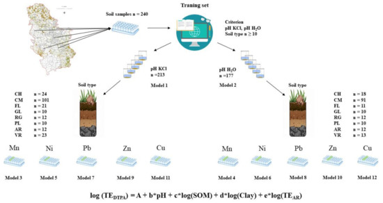
Figure 2.
Schematic diagram of strategy for forming prediction models by soil types. CH–Chernozem; CM–Cambisol; FL–Fluvisol; GL–Gleysol; RG–Regosol; PL–Planosol; AR–Arenosol; VR-Vertisol.
3. Results and Discussion
3.1. Physicochemical Characteristics of Soil
According to the results obtained for pH value, SOM and clay fraction, the soils covered by this research range from strongly acidic to alkaline reaction, low to extremely high SOM content and very low to high clay content.
Out of 213 soil samples (model 1), 84% of soil samples had an acid reaction (pH in KCl), 44% of samples a high to extremely high SOM content and 69% medium and high content of clay fraction [72], as shown in Table 1. Out of 177 samples (model 2), 41% of samples have high to extremely high SOM content and 79% have medium and high content of clay fraction.

Table 1.
Descriptive statistics of the physicochemical properties of the soil samples tested: Minimum, Maximum, Mean, Median and N (number of soil samples tested) for model 1 and 2.
TEAR values above maximum permittable limits (MPL) (prescribed by the regulations of the Republic of Serbia) [73] were obtained for 39 samples for Ni content, 5 samples for Pb and for 2 samples for Cu content (model 1). Based on the classification of Barrett et al. [74] for TEDTPA, 177 samples had high values of bioavailable Mn, 18 samples of bioavailable Zn, and 198 samples of bioavailable Cu.
In accordance with less tested samples in model 2, fewer samples had TEAR values above MPL (24 samples for Ni content and 1 sample for Cu content) and high TEDTPA values (143 samples for bioavailable Mn content, 8 samples for bioavailable Zn and 164 samples for bioavailable Cu).
3.2. Physicochemical Characteristics by Soil Type
For a clearer insight into the values of basic physicochemical parameters by soil type whose impact on the bioavailability of TEs was examined by prediction models 3–12, the results are shown in Table 2.
Table 2.
Descriptive statistics for the basic physicochemical properties of the soil samples tested by type of soil: Minimum, Maximum, Mean, Median, N (number of soil samples tested) and P (percentage of the soil type in the sample) for model 3–12.
The acid soil reaction was determined for the following soil types: CM (97%), RG (83%), GL and PL (80%), AR (75%), VR (74%), CH (71%) and FL (57%). Soil types with high to very high SOM content in the largest number of samples had GL (80%), CH (79%), and VR (61%), while in other types a significantly smaller number of samples (PL50%, RG 50%, FL 48%, CM 29% and AR 25%). According to the number of samples with a medium and high content of clay fraction, CM (83%), GL (80%), CH (75%), VR (74%), PL (60%) and RG (50%) and FL (29%) were singled out, respectively, while the number of samples in type AR (8%) is significantly smaller, which is characteristic of this soil type. For the formation of prediction models by soil types for pH in water (model 4,6,8,10,12) for types GL, RG, PL and AR, the same number of samples was used as for models by soil types for pH in KCl-in (3,5,7,9,11), so that the percentage of samples with high to extremely high content of organic matter and medium and high content of clay fraction was the same. Soil types CH, CM and FL had a high to extremely high SOM content at a higher percentage of the samples, compared to the pH models in KCl, while medium and high clay fraction content at a higher volume of samples was also shown for VR soil type.
The values of the examined basic physical and chemical parameters of the samples for soil types included in this study are within the values for the given soil types in the territory of RS obtained in previous studies [75,76,77,78].
3.3. Prediction Models
In order to predict the impact of predictive parameters and soil type more accurately on the bioavailability of TEs, based on multiple linear regression we formed two basic models (pH in KCl and water suspension) and models by soil type (also for both suspensions pH values), whose determination coefficients (R2) were compared. Regression coefficients that reached statistical significance at the level of 5% are indicated with * in the tables (Table 3 and Table 4 and Tables 6–15).
Table 3.
Prediction model 1.
Table 4.
Prediction model 2.
The reliability of the basic prediction models (R2), as well as the influence of the examined parameters on bioavailability, are shown in Table 3 (Model 1 for pH value in 1M KCl suspension) and Table 4 (Model 2 for pH in water suspension).
The obtained coefficients of determination for all tested TEs ranged from 0.24 to 0.72 (model 1) and from 0.36 to 0.83 (model 2). The most reliable prediction model for both models was for Cu (R2 = 0.72 and R2 = 0.83). A more reliable prediction model for all TEs, except for Zn, proved to be model 2 (pH in water suspension).
Comparison of Model Reliability from this and Previous Study
The reliability of prediction model 1 from this study was lower for all TEs, except for Zn, while for model 2 it was lower for Pb, Zn and Cu, and higher for Mn and Ni (Table 5). In addition to the difference in the values for the reliability of prediction models, in some models, for certain TEs, a different statistically significant influence of the examined soil parameters on the bioavailability of TEs was obtained. Unlike the models obtained in our previous study [31], in model 1 clay had no statistically significant effect on Ni bioavailability, pH had no significance on Pb bioavailability, while SOM statistically significant affected Zn bioavailability and did not affect Cu bioavailability. For prediction model 2, a change in the statistical significance of the influence of the examined parameters on the bioavailability of TEs was obtained for Mn, Ni and Pb. Soil organic matter had a statistically significant effect on the bioavailability of Mn and Ni, while for Pb it had no significance, in contrast to the prediction model from the previous study [31]. Clay had no statistically significant effect on bioavailability of Mn. In general, bioavailability was affected by all examined predictive soil parameters, but TEAR was a mutual variable for all elements and models from this and previous studies.
Table 5.
Reliability of prediction models expressed by the coefficient of determination (R2) for TEs from this and previous study.
3.4. Prediction Models by Soil Type
3.4.1. Manganese
Prediction models for Mn by soil type are presented in Table 6 and Table 7. Models for soil type AR and VR (model 3) and AR (model 4) did not reach statistical significance for the examined parameters and were therefore rejected. Of the accepted models, the reliability by soil type for model 3 ranged from 0.33 to 0.89 and from 0.32 to 0.91 for model 4. In model 3 for CM, the prediction model had less reliability compared to model 1, while model 4 had lower reliability than model 2 for CM, FL and RG. The most reliable model for Mn by soil type was obtained for GL (models 3 and 4). Observing the statistical significance of the examined parameters on the bioavailability of Mn by soil type in relation to the basic model (model 1), there was a change for the influence of pH value in CM and RG. Unlike model 1, in model 3 clay had no statistically significant effect on the bioavailability of Mn. Pseudo-total forms of TEs in PL had no statistically significant effect. Compared to model 2, in prediction model 4 the pH value did not affect the bioavailability of Mn for the following soil types: CM, FL and RG. Unlike model 2, SOM had no statistically significant effect on the bioavailability of Mn by soil type, in all soil types except CM. The influence of clay on the bioavailability of Mn differed from model 2, as well as the SOM, except for CM and GL. The pseudo-total forms of TEs in CH, PL and VR did not have a statistically significant effect on mobility, unlike in model 2.
Table 6.
Prediction model 3.
Table 7.
Prediction model 4.
3.4.2. Nickel
Prediction models for Ni by soil type are presented in Table 8 and Table 9. Models for soil type PL and AR (model 5) and PL, AR and VR (model 6) did not reach statistical significance for the examined parameters and were therefore rejected. Of the accepted models, the reliability by soil type for model 5 ranged from 0.19 to 0.88 and from 0.52 to 0.87 for model 6. In model 5 for CH the prediction model had lower reliability, in comparison to model 1. The most reliable model for Ni by soil type was obtained for WG (models 5 and 6). Observing the statistical significance of the examined parameters on the bioavailability of Ni by soil type in relation to the initial models (models 1 and 2), there was a change in the influence of pH value so that it did not affect the bioavailability of Ni in GL in models 5 and 6, as well as FL in model 6. In model 1, SOM had no effect on bioavailability, but it had an effect in prediction model 5, for CM and GL. Unlike model 2, in model 6 SOM had no effect, except for GL. Clay had a similar effect. In model 5, clay had a statistically significant effect in GL, RG and VR, while in model 6 it had no effect in CH and FL. In model 5, the pseudo-total forms of TEs in CH and GL had no statistically significant effect, as well as for GL in model 6.
Table 8.
Prediction model 5.
Table 9.
Prediction model 6.
3.4.3. Lead
Prediction models for Pb by soil type are presented in Table 10 and Table 11. Models for soil type PL (model 7) and VR (model 8) did not reach statistical significance for the examined parameters and were rejected. Of the accepted models, the reliability by soil type for model 7 ranged from 0.22 to 0.98 and from 0.44 to 0.98 for model 8. In model 7 for CH, CM and VR the prediction model had lower reliability compared to model 1, and in model 8 CH, CM and PL had lower reliability than in model 2. The most reliable model for Pb by soil type was obtained for GL (models 7 and 8). Unlike model 1, in model 7 for types CH and FL the pH value had an effect on the bioavailability of Pb, and in CH SOM also had an effect. Pseudo-total forms of TEs did not statistically significant affect the bioavailability of CH in model 7. In model 8, for all soil types, the pH value did not statistically significant affect the bioavailability of Pb, unlike in model 2.
Table 10.
Prediction model 7.
Table 11.
Prediction model 8.
3.4.4. Zinc
Prediction models for Zn by soil type are presented in Table 12 and Table 13. Models for soil type GL, RG, PL (model 9) and CH, GL, RG and PL (model 10) did not reach statistical significance for the examined parameters and were rejected. Of the accepted models, the reliability by soil type for model 9 ranged from 0.42 to 0.74 and from 0.49 to 0.60 for model 10. In model 9 for VR, the prediction model had lower reliability compared to model 1. The most reliable model for Zn by soil type was for FL (model 9) and VR (model 10). Unlike model 1, in model 9 the pH value affected the bioavailability of Zn in CH. Soil organic matter and clay had no effect on bioavailability in CH, FL and AR. Pseudo-total forms had no effect on VR bioavailability. In model 10, in contrast to model 2, pH value and SOM had an impact on the bioavailability of CM. Clay had no effect on bioavailability, except for CM.
Table 12.
Prediction model 9.
Table 13.
Prediction model 10.
3.4.5. Copper
Prediction models for Cu by soil type are presented in Table 14 and Table 15. The models for soil type PL (model 11) and CA and PL (model 12) did not reach statistical significance for the examined parameters and were therefore rejected. Of the accepted models, the reliability by soil type for model 11 ranged from 0.47 to 0.94 and from 0.54 to 0.94 for model 12. In model 11 for CH, FL and VR the prediction model had lower reliability compared to model 1, and for FL and VR in model 12 compared to model 2. The most reliable model for Cu by soil type was obtained for GL and RG (models 11 and 12). Unlike prediction model 1, in model 11 the pH value did not affect the bioavailability of Cu in GL, RG and AR, as well as the pseudo-total forms in CH. In model 12, SOM did not affect any soil type and pH value had no effect in FL, GL, RG and AR, unlike in model 2.
Table 14.
Prediction model 11.
Table 15.
Prediction model 12.
Tipping et al. [79] highlighted that general prediction and mapping of the state of TEs in soil requires the formation of large representative data sets. However, many authors obtained more useful information with different statistical effects by dividing the tested data set into groups based on the appropriate researched parameters [53,54,55].
In this research, testing sets were formed for the eight most common types of soil on the territory of RS and the division by extraction means for determining the pH value was performed for each soil type.
Out of the total number of models grouped by soil type, pH suspension, for all TEs (model number = 80), 75% were accepted as reliable for predicting bioavailability, of which 70% had a higher R2 in comparison to the basic models (models 1 and 2), shown in Scheme 1.
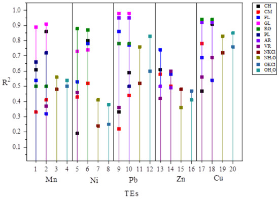
Scheme 1.
Graphic summary of the improvement of prediction model results for bioavailability of TEs by soil type. CH–Chernozem; CM–Cambisol; FL–Fluvisol; GL–Gleysol; RG–Regosol; PL–Planosol; AR–Arenosol; VR–Vertisol; NKCl–basic model, KCl suspension from this study; NH2O-basic model, water suspension from this study; OKCl-basic model, KCl suspension from previous study; OH2O-basic model, water suspension from previous study; 1, 5, 9, 13, 17-Prediction models for TEs by soil type-KCl suspensions from this study; 2, 6, 10, 14, 18-Prediction models for TEs by soil type-water suspensions from this study; 3, 7, 11, 15, 19-Basic prediction models from this study; 4, 8, 12, 16, 20-Basic prediction models from previous study.
By comparing the values of R2 in relation to the basic models of this and a previous study (Table 5. R2 max = 0.85), the models obtained by grouping by soil type for all TEs except Zn had at least one model with R2 greater than 0.85 (17 models in total). Some prediction models for TEs Mn, Pb and Cu had R2 greater than 0.90. Cu proved to be the most reliable, with over 50% of accepted models with R2 greater than 0.90.
Prediction model for FL stood out as one of the most reliable models by soil type, as all models were accepted and more than 50% of models had R2 higher than basic models (models 1 and 2), as well as for CH and CA, where only 1 model was rejected as unreliable (CH for Zn and CA for Cu). The least reliable bioavailability prediction was obtained for PL, where only three models were accepted as statistically significant. For soil type GL and AR, all accepted models had R2 higher than the basic models (eight out of ten models and six out of ten).
By grouping by soil type and comparing the values of R2, model for pH suspension in KCl and water in models where this variable had a statistically significant effect on bioavailability, significantly more reliable models were obtained in water suspension, except for Ni for RG soil type, where the model in 1M KCl was slightly more reliable (Δ R2 = 0.01). By making models for subsets according to the pH range, Zhang et al. [54] obtained more reliable predictions with R2 higher than for basic models. Furthermore, by making models with subsets in relation to the pH value and by including a new parameter, Gandois et al. [53] obtained models with higher reliability, compared to the basic model. In the aforementioned studies, models based on subsets, in addition to more reliable prediction, also showed a change in the statistical significance of certain soil parameters that affect the bioavailability of TEs. Excluding data for soil samples whose types were not included in the testing set of this study changed the reliability of the model in relation to the type of extraction agent for determining the pH value. Based on the obtained results, it can be concluded that predicting the bioavailability of TEs is more reliable using the pH value obtained in the water suspension.
The pseudo-total TEs content had a statistically significant effect on the bioavailability of TEs in the basic models in all five examined TEs, while the influence of pH, clay and SOM was significant for some of the TEs, as shown by the results of our previous study [31]. None of the parameters proved to be the most important for all TEs and soil types for the bioavailability of TEs by soil type.
The number and type of soil parameters that were examined as independent variables varied, but for most soil types it is possible to single out at least one parameter whose impact on bioavailability per soil type is the same for all TEs. Thus, for example, the bioavailability for CH type clay had no statistically significant effect for any TEs, while other variables appeared inconsistent as predictive parameters. The pseudo-total content of TEs had an impact on the bioavailability of the CA type, while SOM and clay did not, and the pH value appeared inconsistent as a predictive parameter. The pseudo-total content of TEs had an impact on the bioavailability of the FL type, while all other variables appeared inconsistent. In type RG, the pseudo-total content of TEs had an effect, while SOM showed no effect. Of the examined variables on bioavailability in the type PL, SOM and clay had no effect, while the prediction of the parameters of pH and pseudo-total amount of TEs was inconsistent by elements. Only the pseudo-total content of TEs was singled out as a predictive parameter in type AR, and pH, SOM and clay had no effect on bioavailability. The prediction of the bioavailability of TEs in most soil types was the function of several predictive parameters, while in the AR-type it was sufficient to use only pseudo-total forms. Sauvé et al. [80] also reported that, in some cases, the prediction of dissolved Cu concentration is more reliable using only total concentrations of that TE.
The results showed that the influence of the predictive parameter depends on the examined element and the soil type.
The pH value affected the bioavailability of most TEs [14], which was in accordance with the study of Carrillo-Gonzales et al. [13], who pointed out that even small changes in pH can strongly affect the solubility of TEs. The mobility and bioavailability of each TE occur within a certain pH range. Outside the given range, the mobility of TEs decreases significantly and at some values immobilization occurs [13,81,82]. The tested soil samples used to form the test set encompassed a wide range of pH values at which TEs can be both mobile and immobilized. It can be assumed that this is one of the reasons for the inconsistency of the influence of pH value on the bioavailability of TEs recorded in this study, but also the fact that the testing set was grouped by soil type, as Naidu and Bolan [83] suggested that pH can have a different impact on the bioavailability of TEs in the soil, with regards to the soil nature.
Many authors have reported that pH has a statistical effect on prediction or is correlated with bioavailable TEs (Mn: [81,84]; Ni: [48,50,54,84]; Pb: [18,48,50,79,85,86]; Zn: [18,50,51,53,79,84,86,87]; Cu: [48,50,53,84,86,88,89]), but also vice versa, that pH had no statistical effect or was not correlated with bioavailable TEs (Mn: [55,89,90,91]; Ni: [51,53,90]; Pb: [51,53,84,90]; Zn: [48,89,90]; Cu: [18,51,56,79,90]).
Soil organic matter accumulates and releases TEs [92], thus acting on the mobilization and immobilization of TEs in the soil [13,42,82]. The high content of SOM has a complex influence on the behaviour of TEs in the soil [82]. Thus, high SOM content (solid) increases cation sorption on the humic matter which reduces the bioavailability of TEs, while high soluble SOM content increases the complexing of the majority of TEs, which can increase and/or decrease the bioavailability of TEs [81]. Likewise, high molecular weight organic compounds form insoluble complexes with TEs which removes them from the solution as they become semi-immobile and by binding to low molecular weight compounds they can remain in solution, which increases their mobility [13]. The double role of SOM on the solubility of TEs is also conditioned by the pH value of the soil. Under very acidic soil conditions, SOM builds insoluble complexes with TEs, making them immobile, and in weakly acidic to alkaline conditions it builds soluble complexes in which TEs are mobile [93]. Han [94] believes that in mineral soils with low SOM content, organic matter increases the bioavailability of TEs, while in organic soils with high SOM content it reduces bioavailability.
The dual effect of SOM on TEs behaviour is obvious, as the results of many studies have shown an effect on TEs prediction or correlation with bioavailable TEs (Mn: [84,89,90]; Ni: [50,53,84,95]; Pb: [51,55,79,86,90]; Zn: [18,50,55,79,89,90]; Cu: [18,50,55,57,86,88,90]) and, vice versa, there are studies in which SOM was not affected or correlated with bioavailable TEs (Mn: [55,56,91]; Ni: [48,51,54,56,90]; Pb: [18,48,50,53,56,57,84]; Zn: [48,51,53,56,57,84,86,87]; Cu: [48,51,53,56,79,84,89]). The influence of SOM on bioavailability in previous literature sources indicates different mechanisms of action of this soil parameter depending on the type of SOM, which is evident from a series of opposite effects in the aforementioned examples. Kabata [82] also points out that in mineral soils the influence of SOM on the behaviour of TEs cannot be expected, since the content of SOM is negligible in relation to the total weight of the soil, while Tack [96] considers that, regardless of the presence of 2% to 10% SOM in mineral soils, it contributes to good structure and plays an important role in physical, chemical and biological processes including the retention of TEs.
In the solid phase of the soil, in addition to SOM, the clay mineral content also has an impact on the behaviour of TEs. The structure of clay minerals may contain a small part of TEs, but the main role in their retention is played by the sorption capacity of clay minerals [82]. Negative charges of clay mineral surfaces are the main contribution to the ability to enable cation exchange, especially in soils with high mineral content [96]. Sorption processes are significantly influenced by the properties of cations and the type of clay minerals [13,97,98,99]. Different chemical composition and structural structure of clay minerals contribute to different TEs’ binding abilities and correlate with cation exchange capacity (CEC). These processes are positively correlated so that, with increasing CEC values, a larger amount of cations is adsorbed on clay minerals [82]. In the most common types of clay minerals, CEC values range in the following order: montmorillonite, imogolite > vermiculite > illite, chlorite > halloysite > kaolinite [82]. High clay content at all pH values in the soil increases the exchange of ions for trace cations, which reduces the bioavailability of TEs, while in soils dominated by the type of clay minerals that have the ability to swell (swelling clays), the bioavailability of TEs is increased [81]. The process of swelling and shrinkage in montmorillonite clay occurs in response to the charge and size of the adsorbed cation between the clay plates. TEs adsorbed by montmorillonite are easily released into the liquid phase of the soil and become bioavailable [82]. In their study, Rékási and Filep linked the impact of solid-phase soil on TEs’ mobility to different characteristics of two land uses, attributing the impact on TEs’ mobility to the organic matter in forest soils and clay in arable land. This is contrary to the opinion of Mahmoudabadi et al. [89] who believe that soil use does not affect clay content, as the soil texture is a constant property, so that the behaviour of TEs is more related to other factors.
Consistent with the results of this study, the results of other studies showed that clay was a statistically significant predictive parameter, or was correlated with bioavailable TEs (Mn: [56,89]; Ni: [56,96,100,101]; Pb: [55,90]; Zn: [48,55,89,90]; Cu: [55,56,57,84,89]) but, on the contrary, it had no effect on prediction or was not correlated (Mn: [55,56,84,90]; Ni: [48,54,56,84,90]; Pb: [48,56,57,84]; Zn: [56,57,84]; Cu: [48,56,90]), which depended on TEs and set research hypotheses.
Aqua regia digestion is used to determine the content of chemical elements in the soil in order to solve environmental problems and it is wrong to describe the elements extracted in aqua regia as total TEs contents, although in some cases their amounts do not differ much from total HF digestion contents [102]. Using the predictive parameter of pseudo-total forms, it is impossible to indicate the origin of the examined TEs, and Kabata [103] indicates that its behaviour (bioavailability) in the soil depends on the origin of TEs. According to Kabata [103], TEs in the solid phase of soils of lithogenic origin are very slight bioavailable, whereas pedogenetic soils and anthropogenic soils are slightly and moderately bioavailable, respectively. In soil solution, TEs of pedogenetic and anthropogenic origin are easily soluble and are highly bioavailable. Due to the lack of insight into the qualitative and quantitative analysis of the origin of the tested TEs in the soil samples of the testing set of this study, no reasonable conclusion can be made about the inconsistent impact of this predictive parameter on the bioavailability of TEs. In the results of other studies, it was shown that pseudo-total amounts of TES show a prediction of bioavailability or are correlated with bioavailable TEs (Mn: [89,91]; Ni: [50,51,54]; Pb: [18,50,51,53,57,85]; Zn: [18,50,57,86,89]; Cu: [18,50,51,53,57,86,88,89]), but also vice versa, that they had no effect or were not correlated with bioavailable TEs (Ni: [53]; Pb: [86]; Zn: [51,53]).
The results of this study, as well as many others previously cited, confirm the quotation from the beginning of this paper, that the main role in controlling the bioavailability of TEs in the environment is played by soil, and according to Pelfrêne et al. [104] the relationship between TEs and different soil parameters is complex and cannot be represented by a single parameter. The content of TEs differs between soil types and geographical regions since the formation of the soil was influenced by the parent rock and the climatic conditions on which the soil was formed [82]. Soil quality standards should be linked to soil type and its exploitation [103], as the biogeochemical cycles of TEs are greatly accelerated by human activity [15].
4. Conclusions
The results of this study showed that predicting the bioavailability of TEs is specific to element and soil type. By forming a testing set according to the soil type and rejecting models that did not reach statistical significance, models whose predictions were more reliable than basic models were obtained, thus confirming the initial hypothesis. As in our previous study, models for Cu and Pb were distinguished for higher reliability, in comparison to the other TEs and basic models for this TE. Reliability of models by soil type for Cu ranged from 0.47 to 0.94 (KCl suspension) and from 0.54 to 0.94 (water suspension), which is higher in comparison to the previous study (0.76 KCl suspension and 0.85 water suspension). Furthermore, values for Pb were 0.22–0.98 (KCl suspension) and 0.44–0.98 (water suspension). These values were also higher in comparison to the R2 values obtained in the previous study (0.60 KCl suspension and 0.83 water suspension).
Multiple linear regression showed that the best models were obtained for the Fluvisol soil type. For this soil type, all 10 models were accepted as reliable for predicting the bioavailability of TEs. The least reliable prediction was obtained for the Planosol soil type.
The results of this study indicated that none of the prediction parameters had a uniform statistical effect on the bioavailability of TEs by soil type, in contrast to the basic models, which was probably related to the soil type and specific conditions that prevail in it. In order to obtain a reliable prediction of TEs’ bioavailability depending on soil parameters, prediction models must be formed based on a test set by soil type.
In order to improve the performance of prediction models, it is necessary to include and examine the influence of type and form of SOM (total and soluble forms), qualitative and quantitative content of clay minerals, the mutual interaction of TEs, the interaction of TEs with solid soil phase and TEs’ origin (sequential analysis), to quantify TEs by their oxidation status, and to form subgroups based on the pH, which value ranges in accordance to the TEs’ nature (mobility and immobility of TEs). The formation of an extensive testing set also requires the application of other statistical techniques that will be able to adequately analyze patterns and structures hidden in large and high-dimensional data sets. This approach to the formation of a test set will provide algorithms that can be used for machine learning and artificial intelligence, which can be used for application in digital agriculture after its validation.
Author Contributions
Conceptualization, J.M. and Z.D.; methodology, J.M., Z.D., R.P., A.S.-S., D.J.; software, D.J., M.J.; validation, R.P., A.S.-S.; formal analysis, Z.D.; investigation, J.M., Z.D., D.J., M.J.; resources, R.P.; data curation, J.M., Z.D., D.J.; writing—original draft preparation, J.M., Z.D., D.J.; writing—review and editing, R.P., A.S.-S.; visualization, J.M., D.J.; supervision, R.P.; project administration, R.P.; funding acquisition, R.P. All authors have read and agreed to the published version of the manuscript.
Funding
This work is part of the contract number: 451-03-68/2020-14/200011 financially supported by the Ministry of Education, Science and Technological Development of the Republic of Serbia.
Institutional Review Board Statement
Not applicable.
Informed Consent Statement
Not applicable.
Data Availability Statement
Not applicable.
Conflicts of Interest
The authors declare no conflict of interest.
References
- Bradl, H.B. Source and Origins of Heavy Metals. In Heavy Metals in the Environment: Origin, Interaction and Remediation, 1st ed.; Bradl, H.B., Ed.; Elsevier: Amsterdam, The Netherlands, 2005; pp. 1–27. [Google Scholar] [CrossRef]
- Naidu, R.; Kim, K.R. Contaminant fate, dynamics and bioavailability: Biochemical and molecular mechanism at the soil: Root interface. Rev. Cienc. Suelo Nutr. Veg. 2008, 8, 56–63. [Google Scholar] [CrossRef][Green Version]
- Ginzky, H.; Heuser, I.L.; Qin, T.; Ruppel, O.C.; Wegerdt, P. International Yearbook of Soil Law and Policy 2016. Int. Yearb. Soil Law Policy 2017. [Google Scholar] [CrossRef]
- Ginzky, H.; Dooley, E.; Heuser, I.L.; Kasimbazi, E.; Markus, T.; Qin, T. International Yearbook of Soil Law and Policy 2017. Int. Yearb. Soil Law Policy 2018. [Google Scholar] [CrossRef]
- Ginzky, H.; Dooley, E.; Heuser, I.L.; Kasimbazi, E.; Markus, T.; Qin, T. International Yearbook of Soil Law and Policy 2018. Int. Yearb. Soil Law Policy 2019. [Google Scholar] [CrossRef]
- MvV. Annexes Circular on Target Values and Intervention Values for Soil Remediation. In Dutch Target and Intervention Values, 2000 (the New Dutch List); Ministerie van Volkshulsvesting, Ruimtelijke Ordeningen Milieubeheer; Ministry of Housing, Spatial Planning and the Environment: Barendrecht, The Netherlands, 2000; Available online: http://esdat.net/Environmental%20Standards/Dutch/annexS_I2000Dutch%20Environmental%20Standards.pdf (accessed on 21 September 2019).
- Carlon, C.; D’Alessandro, M.; Swartjes, F. Derivation Methods of Soil Screening Values in Europe: A Review of National Procedures towards Harmonisation; Scientific and Technical Research Series; Office for Official Publications of the European Communities: Ispra, Italy, 2007. [Google Scholar]
- Bobrowsky, P.; Paulen, R.; Smedley, P.; Alloway, B.J. Appendix A: International Reference Values. In Essentials of Medical Geology, revised ed.; Selinus, O., Ed.; Springer: Dordrecht, The Netherlands, 2013. [Google Scholar] [CrossRef]
- Official Gazette of Republic of Serbia. Regulation on Limit Values of Polluting, Harmful and Dangerous Substances in Soil; Official Gazette of Republic of Serbia: Belgrade, Serbia, 2018. (In Serbian) [Google Scholar]
- Lamb, D.T.; Ming, H.; Megharaj, M.; Naidu, R. Heavy metal (Cu, Zn, Cd and Pb) partitioning and bioaccessibility in uncontaminated and long-term contaminated soils. J. Hazard. Mater. 2009, 171, 1150–1158. [Google Scholar] [CrossRef]
- Smolders, E.; Oorts, K.; Sprang, P.V.; Schoeters, I.; Janssen, C.R.; McGrath, S.P.; McLaughlin, M.J. Toxicity of trace metals in soil as affected by soil type and aging after contamination: Using calibrated bioavailability models to set ecological soil standards. Environ. Toxicol. Chem. 2009, 28, 1633–1642. [Google Scholar] [CrossRef]
- Robinson, B.H.; Bolan, N.S.; Mahimairaja, S.; Clothier, B.E. Solubility, mobility and bioaccumulation of trace elements: Abiotic processes in the rhizosphere. In Trace Elements in the Environment: Biogeochemistry, Biotechnology, and Bioremediation, 1st ed.; Prasad, M.N.V., Kenneth, S.S., Naidu, R., Eds.; CRC Press: Boca Raton, FL, USA, 2005; pp. 97–110. [Google Scholar] [CrossRef]
- Carrillo-Gonzalez, R.; Simunek, J.; Sebastien, S.; Adriano, D. Mechanisms and pathways of trace element mobility in soils. Adv. Agron. 2006, 91, 111–179. [Google Scholar] [CrossRef]
- Lončarić, Z.; Kadar, I.; Jurković, Z.; Kovačević, V.; Popović, B.; Karalić, K. Heavy metals from farm to fork. In Proceedings of the 47th Croatian and 7th International Symposium on Agriculture, Opatija, Croatia, 13–17 February 2012; Pospišil, M., Ed.; University of Zagreb, Faculty of Agriculture: Zagreb, Croatia, 2012; pp. 14–23, ISBN 978–953–7878–03–0. [Google Scholar]
- Violante, A.; Cozzolino, V.; Perelomov, L.; Caporale, A.; Pigna, M. Mobility and bioavailability of heavy metals and metalloids in soil environments. J. Soil. Sci. Plant Nutr. 2010, 10, 268–292. [Google Scholar] [CrossRef]
- Legrand, P.; Turmel, M.C.; Sauve, S.; Courchesne, F. Speciation and bioavailability of trace metals (Cd, Cu, Ni, Pb, Zn) in the rhizosphere of contaminated soils. In Biogeochemistry of Trace Elements in the Rhizosphere, 1st ed.; Huang, P.M., Gobran, G.R., Eds.; Elsevier: New York, NY, USA, 2005; pp. 261–299. [Google Scholar] [CrossRef]
- Roberts, D.; Nachtegaal, M.; Sparks, D.L. Speciation of metals in soils. In Chemical Processes in Soils, 1st ed.; Tabatabai, M.A., Sparks, D.L., Eds.; Soil Science Society of America: Madison, WI, USA, 2005; pp. 619–654. [Google Scholar] [CrossRef]
- Ivezić, V.; Almås, Å.R.; Singh, B.R. Predicting the solubility of Cd, Cu, Pb and Zn in uncontaminated Croatian soils under different land uses by applying established regression models. Geoderma 2012, 170, 89–95. [Google Scholar] [CrossRef]
- Lehmann, J.; Joseph, S. Biochar for Environmental Management: An introduction. In Biochar for Environmental Management: Science, Technology and Implementation, 2nd ed.; Lehmann, J., Joseph, S., Eds.; Taylor & Francis: London, UK, 2015; pp. 1–14. [Google Scholar] [CrossRef]
- Bhagat, S.K.; Tung, T.M.; Yaseen, Z.M. Development of artificial intelligence for modeling wastewater heavy metal removal: State of the art, application assessment and possible future research. J. Clean. Prod. 2020, 250, 119473. [Google Scholar] [CrossRef]
- Nakamura, K.; Yasutaka, T.; Kuwatani, T.; Komai, T. Development of a predictive model for lead, cadmium and fluorine soil–water partition coefficients using sparse multiple linear regression analysis. Chemosphere 2017, 186, 501–509. [Google Scholar] [CrossRef] [PubMed]
- Ashrafi, M.; Borzuie, H.; Bagherian, G.; Chamjangali, M.A.; Nikoofard, H. Artificial neural network and multiple linear regression for modeling sorption of Pb2+ ions from aqueous solutions onto modified walnut shell. Sep. Sci. Technol. 2020, 55, 222–233. [Google Scholar] [CrossRef]
- Anagu, I.; Ingwersen, J.; Utermann, J.; Streck, T. Estimation of heavy metal sorption in German soils using artificial neural networks. Geoderma 2009, 152, 104–112. [Google Scholar] [CrossRef]
- Imoto, Y.; Yasutaka, T. Comparison of the impacts of the experimental parameters and soil properties on the prediction of the soil sorption of Cd and Pb. Geoderma 2020, 376, 114538. [Google Scholar] [CrossRef]
- Vidal, M.; Santos, M.J.; Abrão, T.; Rodríguez, J.; Rigol, A. Modeling competitive metal sorption in a mineral soil. Geoderma 2009, 149, 189–198. [Google Scholar] [CrossRef]
- Mouni, L.; Belkhiri, L.; Bouzaza, A.; Bollinger, J.C. Interactions between Cd, Cu, Pb, and Zn and four different mine soils. Arab. J. Geosci. 2017, 10, 1–9. [Google Scholar] [CrossRef]
- Campillo-Cora, C.; Conde-Cid, M.; Arias-Estévez, M.; Fernández-Calviño, D.; Alonso-Vega, F. Specific Adsorption of Heavy Metals in Soils: Individual and Competitive Experiments. Agronomy 2020, 10, 1113. [Google Scholar] [CrossRef]
- Xiao, H.; Böttcher, J.; Utermann, J. Evaluation of field-scale variability of heavy metal sorption in soils by scale factors—Scaling approach and statistical analysis. Geoderma 2015, 241–242, 115–125. [Google Scholar] [CrossRef]
- Ming, H.; Naidu, R.; Sarkar, B.; Lamb, D.T.; Liu, Y.; Megharaj, M.; Sparks, D. Competitive sorption of cadmium and zinc in contrasting soils. Geoderma 2016, 268, 60–68. [Google Scholar] [CrossRef]
- Di Bonito, M.; Lofts, S.; Groenenberg, J.E. Models of geochemical speciation: Structure and applications. In Environmental Geochemistry; De Vivo, B., Belkin, H.E., Lima, A., Eds.; Elsevier: Amsterdam, The Netherlands, 2018; pp. 237–305. [Google Scholar] [CrossRef]
- Dinić, Z.; Maksimović, J.; Stanojković-Sebić, A.; Pivić, R. Prediction Models for Bioavailability of Mn, Cu, Zn, Ni and Pb in Soils of Republic of Serbia. Agronomy 2019, 9, 856. [Google Scholar] [CrossRef]
- Trakal, L.; Komárek, M.; Száková, J.; Zemanová, V.; Tlustoš, P. Biochar application to metal-contaminated soil: Evaluating of Cd, Cu, Pb and Zn sorption behavior using single- and multi-element sorption experiment. Plant. Soil. Environ. 2011, 57, 372–380. [Google Scholar] [CrossRef]
- Janssen, R.P.T.; Peijnenburg, W.J.G.M.; Posthuma, L.; Van Den Hoop, M.A.G.T. Equilibrium partitioning of heavy metals in dutch field soils. I. Relationship between metal partition coefficients and soil characteristics. Environ. Toxicol. Chem. 1997, 16, 2470–2478. [Google Scholar] [CrossRef]
- Cambier, P.; Michaud, A.; Paradelo, R.; Germain, M.; Mercier, V.; Guérin-Lebourg, A.; Revallier, A.; Houot, S. Trace metal availability in soil horizons amended with various urban waste composts during 17 years—Monitoring and modelling. Sci. Total Environ. 2019, 651, 2961–2974. [Google Scholar] [CrossRef] [PubMed]
- Degryse, F.; Smolders, E.; Parker, D.R. Partitioning of metals (Cd, Co, Cu, Ni, Pb, Zn) in soils: Concepts, methodologies, prediction and applications—A review. Eur. J. Soil. Sci. 2009, 60, 590–612. [Google Scholar] [CrossRef]
- Hu, B.; Xue, J.; Zhou, Y.; Shao, S.; Fu, Z.; Li, Y.; Chen, S.; Qi, L.; Shi, Z. Modelling bioaccumulation of heavy metals in soil-crop ecosystems and identifying its controlling factors using machine learning. Environ. Pollut. 2020, 262, 114308. [Google Scholar] [CrossRef] [PubMed]
- Viala, Y.; Laurette, J.; Denaix, L.; Gourdain, E.; Méléard, B.; Nguyen, C.; Schneider, A.; Sappin-Didier, V. Predictive statistical modelling of cadmium content in durum wheat grain based on soil parameters. Environ. Sci. Pollut. Res. 2017, 24, 20641–20654. [Google Scholar] [CrossRef]
- Ivezić, V.; Almås, Å.R.; Singh, B.R.; Lončarić, Z. Prediction of trace metal concentrations (Cd, Cu, Fe, Mn and Zn) in wheat grain from unpolluted agricultural soils. Acta Agric. Scand. Sect. B Soil Plant Sci. 2013, 63, 360–369. [Google Scholar] [CrossRef]
- Kader, M.; Lamb, D.T.; Wang, L.; Megharaj, M.; Naidu, R. Predicting copper phytotoxicity based on pore-water pCu. Ecotoxicology 2016, 25, 481–490. [Google Scholar] [CrossRef]
- Versluijs, C.W.; Otte, P.F. Accumulation of Metals in Plants. In A Contribution to the Technical Evaluation of the Intervention Values and Site-Specific Risk Assessment of Contaminated Sites; RIVM report 711701024; National Institute for Public Health and the Environment: Bilthoven, The Netherlands, 2001. [Google Scholar]
- Zhang, H.; Yin, S.; Chen, Y.; Shao, S.; Wu, J.; Fan, M.; Chen, F.; Gao, C. Machine learning-based source identification and spatial prediction of heavy metals in soil in a rapid urbanization area, eastern China. J. Clean. Prod. 2020, 273, 122858. [Google Scholar] [CrossRef]
- Martíne, I.; Maria, A.; Bernal, P. Environmental Impact of Metals, Metalloids, and Their Toxicity. In Metalloids in Plants: Advances and Future Prospects, 1st ed.; Deshmukh, R., Tripathi, D.K., Guerriero, G., Eds.; John Wiley & Sons: Hoboken, NJ, USA, 2020; pp. 451–488. [Google Scholar] [CrossRef]
- Baize, D.; Bellanger, L.; Tomassone, R. Relationships between concentrations of trace metals in wheat grains and soil. Agron. Sustain. Dev. 2009, 29, 297–312. [Google Scholar] [CrossRef]
- Sarkar, S.; Sarkar, B.; Basak, B.B.; Mandal, S.; Biswas, B.; Srivastava, P. Soil Mineralogical Perspective on Immobilization/Mobilization of Heavy Metals. In Adaptive Soil Management: From Theory to Practices, 1st ed.; Rakshit, A., Abhilash, P.C., Singh, H.B., Ghosh, S., Eds.; Springer: Singapore, 2017; pp. 89–102. [Google Scholar] [CrossRef]
- Otte, P.F.; Lijzen, J.P.A.; Otte, J.G.; Swartjes, F.A.; Versluijs, C.W. Evaluation and Revision of the C Soil Parameter Set; RIVM Report 711701021; National Institute of Public Health and the Environment: Bilthoven, The Netherlands, 2001. [Google Scholar]
- Krauss, M.; Wilcke, W.; Kobza, J.; Zech, W. Predicting heavy metal transfer from soil to plant: Potential use of Freundlich-type function. J. Plant Nutr. Soil. Sci. 2002, 165, 3–8. [Google Scholar] [CrossRef]
- Liang, Z.; Ding, Q.; Wei, D.; Li, J.; Chen, S.; Maa, Y. Major controlling factors and predictions for cadmium transfer from the soil into spinach plants. Ecotoxicol. Environ. Saf. 2013, 93, 180–185. [Google Scholar] [CrossRef] [PubMed]
- De Souza Braz, A.M.; Fernandes, A.R.; Ferreira, J.R.; Alleoni, L.R.F. Distribution coefficients of potentially toxic elements in soils from the eastern Amazon. Environ. Sci. Pollut. Res. 2013, 20, 7231–7242. [Google Scholar] [CrossRef] [PubMed]
- Buchter, B.; Davido, B.; Amacher, M.C.; Hinz, C.; Iskandar, I.K.; Selim, H.M. Correlation of Freundlich Kd and n retention parameters with soils and elements. Soil. Sci. 1989, 148, 370–379. [Google Scholar] [CrossRef]
- Sauvé, S.; Hendershot, W.; Allen, H.E. Solid-Solution Partitioning of Metals in Contaminated Soils: Dependence on pH, Total Metal Burden, and Organic Matter. Environ. Sci. Technol. 2000, 34, 1125–1131. [Google Scholar] [CrossRef]
- Sauvé, S.; Manna, S.; Turmel, M.C.; Roy, A.G.; Courchesne, F. Solid−Solution Partitioning of Cd, Cu, Ni, Pb, and Zn in the Organic Horizons of a Forest Soil. Environ. Sci. Technol. 2003, 37, 5191–5196. [Google Scholar] [CrossRef]
- Kashem, A.; Singh, B.R. Solid-Phase Speciation of Cd, Ni, and Zn in Contaminated and Noncontaminated Tropical Soils. In Trace Elements in Soil: Bioavailability, Flux, and Transfer; Iskandar, I.K., Kirkham, M.B., Eds.; Lewis Publishers: Boca Raton, FL, USA; London, UK; New York, NY, USA; Washington, DC, USA, 2001; pp. 213–228. ISBN 9780429137907. [Google Scholar] [CrossRef]
- Gandois, L.; Probst, A.; Dumat, C. Modelling trace metal extractability and solubility in French forest soils by using soil properties. Eur. J. Soil Sci. 2010, 61, 271–286. [Google Scholar] [CrossRef]
- Zhang, X.; Li, J.; Wei, D.; Li, B.; Ma, Y. Predicting Soluble Nickel in Soils Using Soil Properties and Total Nickel. PLoS ONE 2015, 10, e0133920. [Google Scholar] [CrossRef]
- Jahiruddin, M.; Harada, H.; Hatanaka, T.; Islam, M.R. Status of trace elements in agricultural soils of Bangladesh and relationship with soil properties. Soil. Sci. Plant. Nutr. 2000, 46, 963–968. [Google Scholar] [CrossRef]
- Rékási, M.; Filep, T. Factors determining Cd, Co, Cr, Cu, Ni, Mn, Pb and Zn mobility in uncontaminated arable and forest surface soils in Hungary. Environ. Earth. Sci. 2015, 74, 6805–6817. [Google Scholar] [CrossRef]
- De Vries, W.; Curlik, J.; Muranyi, A.; Alloway, B.; Groenenberg, B.J. Assessment of relationships between total and reactive concentrations of cadmium, copper, lead and zinc in Hungarian and Slovakian soils. Ekol. Bratisl. 2005, 24, 152–169. [Google Scholar]
- Ivezić, V. Trace Metal Availability in Soils under Different Land Uses of the Danube Basin in Croatia. Ph.D. Thesis, Department of Plant and Environmental Sciences, Norwegian University of Life Sciences, As, Norway, October 2011. [Google Scholar]
- Moreira, C.S.; Alleoni, L.R.F. Adsorption of Cd, Cu, Ni and Zn in tropical soils under competitive and non-competitive systems. Sci. Agric. 2010, 67, 301–307. [Google Scholar] [CrossRef][Green Version]
- Weng, L.P.; Wolthoorn, A.; Lexmond, T.M.; Temminghoff, E.J.M.; van Riemsdijk, W.H. Understanding the Effects of Soil Characteristics on Phytotoxicity and Bioavailability of Nickel Using Speciation Models. Environ. Sci. Technol. 2004, 38, 156–162. [Google Scholar] [CrossRef] [PubMed]
- Bradl, H.B. Adsorption of heavy metal ions on soils and soils constituents. J. Colloid Interface Sci. 2004, 277, 1–18. [Google Scholar] [CrossRef]
- Zemanová, V.; Trakal, L.; Ochecová, P.; Száková, J.; Pavlíková, D. A model experiment: Competitive sorption of Cd, Cu, Pb and Zn by three different soils. Soil Water Res. 2014, 9, 97–103. [Google Scholar] [CrossRef]
- Sahraoui, H.; Andrade, M.L.; Hachicha, M.; Vega, F.A. Competitive sorption and desorption of trace elements by Tunisian Aridisols Calcorthids. Environ. Sci. Pollut. Res. 2015, 22, 10861–10872. [Google Scholar] [CrossRef]
- Palansooriya, K.N.; Shaheen, S.M.; Chen, S.S.; Tsang, D.C.W.; Hashimoto, Y.; Hou, D.; Bolan, N.S.; Rinklebe, J.; Ok, Y.S. Soil amendments for immobilization of potentially toxic elements in contaminated soils: A critical review. Environ. Int. 2020, 134, 105046. [Google Scholar] [CrossRef]
- Vidojević, D.; Manojlović, M.; Đorđević, A.; Nešić, L.J.; Dimić, B. Estimation of soil organic carbon stock in the Republic of Serbia. In Proceedings of the 2nd International and 14th National Congress of Soil Science Society of Serbia, Solutions and Projections for Sustainable Soil Management, Novi Sad, Serbia, 25–28 September 2017; pp. 154–159, ISBN 978-86-912877-1-9. [Google Scholar]
- Hadžić, V.; Nešić, L.J.; Belić, M.; Furman, T.; Savin, L. Potential of soils in Serbia. Tract. Power Mach. 2002, 7, 43–51. [Google Scholar]
- Official Gazette of Republic of Serbia. Spatial Planning Law of the Republic of Serbia from 2010 to 2020; No. 88; Official Gazette of Republic of Serbia: Belgrade, Serbia, 2010. (In Serbian) [Google Scholar]
- European Environment Agency (EEA). CORINE Land Cover. 2018. Available online: https://land.copernicus.eu/pan-european/corine-land-cover (accessed on 14 July 2020.).
- Mrvić, V.; Antonović, G.; Čakmak, D.; Perović, V.; Maksimović, S.; Saljnikov, E.; Nikoloski, M. Pedological and pedogeochemical map of Serbia. In Proceedings of the 1st International Congress on Soil Science, XIII National Congress in Soil Science: Soil-Water-Plant, Belgrade, Serbia, 23–26 September 2013; pp. 93–105. [Google Scholar]
- Škorić, A.; Filipovski, G.; Ćirić, M. Classification of Yugoslav Soils, special ed.; Book 78; Academy of Sciences and Arts of Bosnia and Herzegovina: Sarajevo, Bosnia and Herzegovina, 1985; p. 72, (In Serbo-Croatian). [Google Scholar]
- Harmonization of the Nomenclature of the Basic Pedological Map with WRB Classification; Faculty of Forestry, University of Belgrade: Belgrade, Serbia, 2011. (In Serbian)
- Edwards, A.C. Interpreting Soil Test Results: What Do All the Numbers Mean? 3rd ed.; CSIRO Publishing: Clayton, Australia, 2016; p. 200. ISBN 9781486303960. [Google Scholar]
- Official Gazette of Republic of Serbia. Rule Book of Allowed Concentrations of Dangerous and Hazardous Materials in Soil and in Water for Irrigation and Methods for Analysis; No. 23; Official Gazette of Republic of Serbia: Belgrade, Serbia, 1994. (In Serbian) [Google Scholar]
- Barrett, W.; Jones, N.; Chu, P.; Pohlman, K.; Coleman, G.; Poole, H.; Go, D.; Spiva, C.; Grith, L.; Zwiep, J.; et al. Micronutrients. In Agronomy Handbook, Soil and Plant analysis Resource Handbook; Ankerman, D., Large, R., Eds.; Midwest Laboratories, INC: Omaha, NE, USA, 2017; pp. 65–76. [Google Scholar]
- Pavlović, P.; Kostić, N.; Karadžić, B.; Mitrović, M. The Soils of Serbia; World Soils Book Series; Springer Science+Business Media: Dordrecht, The Netherlands, 2017; p. 233. [Google Scholar] [CrossRef]
- Tanasijević, Đ.; Pavićević, N.; Antonović, G.; Filipović, Đ.; Aleksić, Ž.; Spasojević, M. Pedological Cover of Western and Northwestern Serbia; Institute of Soil Science: Belgrade, Serbia, 1966. (In Serbian) [Google Scholar]
- Pavićević, N.; Nikodijević, V.; Antonović, G.; Tanasijević, Đ. Soils of Stari Vlah and Raska; Institute of Soil Science: Belgrade, Serbia, 1968. (In Serbian) [Google Scholar]
- Antonović, G.; Pavićević, N.; Nikodijević, V.; Aleksić, Ž.; Tanasijević, Đ.; Filipović, Đ.; Vojinović, L.J.; Jeremić, M. Soil of the Timok Basin; Institute of Soil Science: Belgrade, Serbia, 1974. (In Serbian) [Google Scholar]
- Tipping, E.; Rieuwerts, J.; Pan, G.; Ashmore, M.R.; Lofts, S.; Hill, M.T.R.; Farago, M.E.; Thornton, I. The solid–solution partitioning of heavy metals (Cu, Zn, Cd, Pb) in upland soils of England and Wales. Environ. Pollut. 2003, 125, 213–225. [Google Scholar] [CrossRef]
- Sauvé, S.; McBride, M.; Norvell, W.A.; Hendershot, W. Copper Solubility and Speciation of In Situ Contaminated Soils: Effects of Copper Level, pH and Organic Matter. Water Air Soil Pollut. 1997, 100, 133–149. [Google Scholar] [CrossRef]
- Adriano, D.C. Trace Elements in Terrestrial Environments: Biogeochemistry, Bioavailability, and Risks of Metals, 2nd ed.; Springer: Berlin/Heidelberg, Germany, 2001; ISBN 978-0-387-21510-5. [Google Scholar] [CrossRef]
- Kabata-Pendias, A. Trace Elements in Soils and Plants, 4th ed.; CRC Press; Taylor & Francis Group: Boca Raton, FL, USA, 2010; ISBN 9781420093681. [Google Scholar] [CrossRef]
- Naidu, R.; Bolan, N.S. Contaminant chemistry in soils: Key concepts and bioavailability. In Developments in Soil Science; Hartemink, A.E., McBratney, A.B., Naidu, R., Eds.; Elsevier: Amsterdam, The Netherlands, 2008; pp. 9–37. [Google Scholar] [CrossRef]
- Sungur, A.; Soylak, M.; Ozcan, H. Investigation of heavy metal mobility and availability by the BCR sequential extraction procedure: Relationship between soil properties and heavy metals availability. Chem. Speciat. Bioavailab. 2014, 26, 219–230. [Google Scholar] [CrossRef]
- Jopony, M.; Young, S.D. The solid solution equilibria of lead and cadmium in polluted soils. Eur. J. Soil Sci. 1994, 45, 59–70. [Google Scholar] [CrossRef]
- McBride, M.; Sauve, S.; Hendershot, W. Solubility control of Cu, Zn, Cd and Pb in contaminated soils. Eur. J. Soil Sci. 1997, 48, 337–346. [Google Scholar] [CrossRef]
- Rutkowska, B.; Szulc, W.; Bomze, K.; Gozdowski, D.; Spychaj-Fabisiak, E. Soil factors afecting solubility and mobility of zinc in contaminated soils. Int. J. Environ. Sci. Technol. 2015, 12, 1687–1694. [Google Scholar] [CrossRef]
- Mondaca, P.; Neaman, A.; Sauvé, S.; Salgado, E.; Bravo, M. Solubility, partitioning, and activity of copper-contaminated soils in a semiarid region. J. Plant Nutr. Soil Sci. 2015, 178, 452–459. [Google Scholar] [CrossRef]
- Mahmoudabadi, E.; Sarmadian, F.; Nazary Moghaddam, R. Spatial distribution of soil heavy metals in diferent land uses of an industrial area of Tehran (Iran). Int. J. Environ. Sci. Technol. 2015, 12, 3283–3298. [Google Scholar] [CrossRef]
- Dragović, S.; Mihailović, N.; Gajić, B. Heavy metals in soils: Distribution, relationship with soil characteristics and radionuclides and multivariate assessment of contamination sources. Chemosphere 2008, 72, 491–495. [Google Scholar] [CrossRef]
- Behera, S.K.; Shukla, A.K. Total and Extractable Manganese and Iron in Some Cultivated Acid Soils of India: Status, Distribution and Relationship with Some Soil Properties. Pedosphere 2014, 24, 196–208. [Google Scholar] [CrossRef]
- Mleczek, M.; Gąsecka, M.; Kaniuczak, J.; Goliński, P.; Szostek, M.; Magdziak, Z.; Rutkowski, P.; Budzyńska, S. Dendroremediation: The Role of Trees in Phytoextraction of Trace Elements. In Phytoremediation; Ansari, A.A., Gill, S.S., Gill, R., Lanza, G.R., Newman, L., Eds.; Springer: Cham, Switzerland, 2018; pp. 269–295. ISBN 978-3-319-99650-9. [Google Scholar] [CrossRef]
- Brümmer, G.W. Heavy Metal Species, Mobility and Availability in Soils. In The Importance of Chemical “Speciation” in Environmental Processes; Bernhard, M., Brinckman, F.E., Sadler, P.J., Eds.; Springer: Berlin/Heidelberg, Germany, 1986; Volume 33, pp. 169–192. ISBN 978-3-642-70443-7. [Google Scholar] [CrossRef]
- Han, F.X. Biogeochemistry of Trace Elements in Arid Environments; Springer: Cham, Switzerland; Dordrecht, The Netherlands, 2007; ISBN 978-1-4020-6024-3. [Google Scholar] [CrossRef]
- Kabata-Pendias, A.; Mukherjee, A.B. Trace Elements from Soil to Human; Springer: Berlin/Heidelberg, Germany, 2007; p. 17. ISBN 978-3-540-32714-1. [Google Scholar] [CrossRef]
- Tack, F.G. Trace elements: General soil chemistry, principles and processes. In Trace Elements in Soils; Hooda, P.S., Ed.; John Wiley and Sons: Chichester, UK, 2010. [Google Scholar] [CrossRef]
- Abd-Elfattah, A.; Wada, K. Adsorption of lead, copper, zinc, cobalt, and cadmium by soils that differ in cation-exchange materials. J. Soil Sci. 1981, 32, 271–283. [Google Scholar] [CrossRef]
- Tiller, K.G.; Gerth, J.; Brümmer, G. The relative affinities of Cd, Ni and Zn for different soil clay fractions and goethite. Geoderma 1984, 34, 17–35. [Google Scholar] [CrossRef]
- Helios Rybicka, E.; Calmano, W.; Breeger, A. Heavy metals sorption/desorption on competing clay minerals; an experimental study. Appl. Clay Sci. 1995, 9, 369–381. [Google Scholar] [CrossRef]
- Hseu, Z.Y.; Chen, Z.S. Nickel in Serpentine Soils. In Nickel in Soils and Plants; Tsadilas, C., Rinklebe, J., Selim, M., Eds.; CRC Press; Taylor & Francis Group: Boca Raton, FL, USA, 2018; pp. 181–198. ISBN 978-1498774604. [Google Scholar] [CrossRef]
- Nikoli, T.; Matsi, T. Methods of Ni Determination in Soils and Plants. In Nickel in Soils and Plants; Tsadilas, C., Rinklebe, J., Selim, M., Eds.; CRC Press; Taylor & Francis Group: Boca Raton, FL, USA, 2018; pp. 199–216. ISBN 9781498774604. [Google Scholar] [CrossRef]
- Taraškevičius, R.; Zinkutė, R.; Stakėnienė, R.; Radavičius, M. Case Study of the Relationship between Aqua Regia and Real Total Contents of Harmful Trace Elements in Some European Soils. J. Chem. 2013, 1–15. [Google Scholar] [CrossRef]
- Kabata-Pendias, A. Soil plant transfer of trace elements—An environmental issue. Geoderma 2004, 122, 143–149. [Google Scholar] [CrossRef]
- Pelfrêne, A.; Gassama, N.; Grimaud, D. Mobility of major-, minor- and trace elements in solutions of a planosolic soil: Distribution and controlling factors. App. Geochem. 2009, 24, 96–105. [Google Scholar] [CrossRef]


Publisher’s Note: MDPI stays neutral with regard to jurisdictional claims in published maps and institutional affiliations. |
© 2021 by the authors. Licensee MDPI, Basel, Switzerland. This article is an open access article distributed under the terms and conditions of the Creative Commons Attribution (CC BY) license (http://creativecommons.org/licenses/by/4.0/).