NRC Designs—New Tools for Successful Agricultural Experiments

Abstract

In a nested row–column design (NRC), the experimental units in each of n blocks are grouped into $n_1$ rows and $n_2$ columns. Due to its structure, this experimental design allows full control of the experimental material and a relatively simple feedback loop within the “statistical triangle”. By applying such designs in agricultural experiments, we provide an insurance policy against future unexpected problems. Until now, the cost of this policy has been a complex statistical analysis of experimental data. This paper proposes a new “direct” approach to ANOVA based on the latest literature on the subject. The paper provides the theoretical foundations of this approach, indicates the possibility of applying it to factorial and near-factorial experiments, and supplements the theory with a familiar letter-based representation of all-pairwise comparisons, which has so far been lacking in the literature. The methodology is illustrated by the analysis of a field experiment carried out to improve the use of fungicides against late blight in tomato processing. The presented analytical tools are supplemented with code in R.

1. Introduction

Although almost 100 years have passed since Fisher published the basic principles of experimental planning, it remains one of the most important problems faced by biologists and statisticians [1,2,3]. Only proper planning and adequate analysis of experimental data can be a guarantee of success—a guarantee that the expenditure incurred will enable the formulation of correct and satisfactory conclusions regarding the research problems addressed.

In agricultural comparative experiments we conventionally follow the general theory of scientific research, the heart of which is the “statistical triangle” described by Hinkelmann and Kempthorne [4] and extended by Casler [5]. The starting point in conducting experiments is to pose questions and formulate hypotheses, which should be transcribed to models based on a specific topic (e.g., tomatoes) and then translated into a statistical model and developed in conjunction with statistical design (see Figure 1). The data obtained in the experiment, after being subjected to an analysis determined by the researcher’s previous assumptions, constitute a basis for formulating conclusions regarding the research problems addressed, usually to determine the influence of the studied treatments on the observed variable [6]. At this point, when the process seems complete, a feedback loop should appear, as a good experiment usually leads to more questions and hypotheses. The acquired knowledge should be used to answer new biological and statistical questions, which will increase the effectiveness of the experiments [5].

One of the prerequisites for success is to incorporate the structure of the experimental material into the experimental design so that the results are not distorted, for example by soil variability. Even seemingly homogeneous fields can give heterogeneous answers [7]. In the literature, therefore, it is proposed to use bidirectional blocking in field experiments as an insurance policy, especially if the statistical analysis is to be based on the analysis of variance. In this paper, it is proposed to use nested row–column designs, which provide a powerful structural base for the two-dimensional control of experimental trends [8], and also give the possibility of a relatively simple feedback loop (Figure 1). Experiments with multiple blocking structures are usually carried out using a mixed-model specification, which in the classical approach leads to the analysis of variance in the strata [8,9]. Unfortunately, the inconvenience of inference (see Section 2) in this approach can demotivate the use of safe design solutions. Motivated by the latest publications on the direct approach to ANOVA [10,11,12,13], I suggest applying this modern approach to the analysis of experiments laid out as NRC designs. The available literature on this topic requires the reader to have an advanced mathematical apparatus. For that reason, this paper refers only to those elements of direct ANOVA that are relevant from the practical point of view.

The aim of the paper is to present and illustrate a complete set of analytical tools that make it possible to carry out direct inference in a nested row–column design under a randomization-derived mixed model of observations. Moreover, to the best of my knowledge, for these designs, there is no package or statistical program that can run the described procedure. For this reason, the article has been supplemented with R code and procedures (Appendix A).

The paper is organized as follows. Section 2 describes three basic principles of an insurance policy in agricultural experiments. Section 3 begins with introduction of the NRC designs and presents the randomization-derived mixed model of observations, then gives the theoretical background of the analysis under the direct approach. The section ends by showing how to proceed with the analysis for the very common treatment factorial experiments, and a novel letter-based procedure for all-pair comparisons is proposed. A detailed analysis of a field experiment carried out to improve the use of fungicides against late blight in tomato processing, using the proposed approach, is presented in Section 4. The paper ends with a discussion in Section 5.

2. Insurance Policy in Agricultural Experiments

It should be remembered that statistical design consists of equal measure of treatment design and experimental design. Treatment design is responsible for the arrangement of treatments on experimental units, and sets up a theoretical plan by which the treatment levels are arranged in the experiment. The choice of a plan is related to the definition of the experimental factors and control treatments as well as the technical possibilities related to the methodology of conducting the research and the manner of observation and data collection. The problem of choosing a plan for different types of experiments has been discussed in numerous publications. For instance, some methods of designing factorial experiments with a control treatment in a block design with nested rows and columns are widely considered by Bailey and Łacka [14] and Bose and Mukerjee [15]. An example of this type of experiments is also presented in Section 4. Note the different number of replicates for the control compared to the rest of the treatments in the experiment considered there, which is often found in theoretical plans of experiments with a control treatment and multiple blocking structures [16].

Experimental design should be based on the principles of replication, randomization and local control, i.e., blocking. When planning an experiment, all these principles must be considered from the point of view of its purpose and the conditions under which the experiment is to be carried out, due to their fundamental influence on the analysis of the experimental data and further inference [9].

The principle of replication, i.e., the use of a treatment on several experimental units, is commonly known. It is well known that replication provides the possibility of estimating the experimental error affecting the observation. It is thanks to replication that we obtain greater precision in the estimation of treatment effects or their comparisons. In general, the standard error of the estimator of effects decreases with an increase in the number of replications; however, the use of a large number of repetitions for each treatment can make it difficult to ensure the homogeneity of the experimental material. This fact should not always be viewed as a disadvantage, as such heterogeneity may reflect the natural variability of the population that we infer from the experiment. Thus, replication contributes to an increase in the representativeness of the experimental material.

In the accepted theory, blocking should be related to the earlier recognition of the directions of variability of the material used in the experiment, and lead to a grouping of the experimental units into a system of blocks such that the units inside the blocks are as homogeneous as possible. Local control is commonly used for field trials and plant protection trials carried out under found conditions; however, as research has shown, it should also be included in greenhouse experiments. Hartung et al. [17] indicate blocking as more efficient in improving the precision of greenhouse experiments than the re-arrangement of pots, and hence they recommend it for comparative greenhouse experiments. On the other hand, Casler [5] points to the “dark side” of blocking, noting that block designs in which blocks are linearly arranged without prior recognition of spatial variation can seriously reduce the likelihood of success of the experiment. Taking into account the fact that many experimental stations have visually homogeneous fields, the author suggests the use of two-way blocking as a kind of insurance policy against erroneous blocking. It has been proposed in the literature to use many different designs to control two sources of external variation, such as Latin squares, Youden squares, generalized Youden designs, or row–column designs. Unfortunately, most of these designs are characterized by several important constraints: Youden squares and generalized Youden designs exist only for a limited number of parameter combinations, hence their practical application is limited. On the other hand, row–column designs can have row–column interaction problems when multiple rows and columns are used. Moreover, neither of these designs are applicable to the analysis of a series of experiments carried out, for example, in different locations. An excellent answer to these constraints are nested row–column (NRC) designs, i.e., designs in which in each of n blocks, $n_1{n}_2$ experimental units are grouped into $n_1$ rows and $n_2$ columns [8,12,18]. These experimental designs, which are a natural extension of the previously introduced row–column designs, enable not only full control of the experimental material, but also a relatively simple feedback loop and the making of modifications within the “statistical triangle” when the experimental setup turns out to be “overestimated” and the block insurance policy is exaggerated or other unexpected problems arise in the course of the experiment. Moreover, as Chang and Notz [19] note, for a given number of experimental units, NRC designs have fewer rows and columns per block. The row–column interactions in the NRC designs are likely not as severe as in row–column designs. Therefore, NRC designs are particularly useful for eliminating heterogenity in two directions when there are row and column interactions.

In field experiments, it is worth taking into account the possibility of loss of some of the biological material as a result of unforeseen weather conditions, such as flooding or hail, which may destroy some plots or the entire experiment. If, as a result of such events, only one block of research material is obtained, it will still be possible to analyze it in a row–column design.

If the experimental material turns out to be homogeneous within a range of rows or columns, ignoring the system of rows (columns) leaves the system of blocks and the system of columns (rows), forming a nested block design or—in a very specific situation for two-factorial experiments—a split-plot design [13].

Ignoring any two of the systems—blocks and rows or blocks and columns or rows and columns—still leaves a proper block design. Of course, any decision to ignore the previously considered blocking must have a biological and statistical basis [20].

Another insurance policy, no less important than blocking, is the two-level randomness principle. The first level concerns sampling from a previously defined population so as to ensure the representativeness of the sample. The second level concerns the arrangement of treatments on experimental units. Thus, randomization is a way to eliminate the bias of measurements performed due to systematic differences between experimental units. Unbias is perhaps the most important goal of randomizing plots before assigning them to treatments, ensuring that certain treatments are not continually favored or harmed by random sources of variation in the experimental material and the environment. Moreover, randomization introduces randomness into the existing variability of experimental units. With randomization, a properly performed statistical analysis of the experimental results becomes correct, assuming that in deriving this analysis, the randomization is fully taken into account [21]. In the case of NRC designs, the randomization scheme is performed by randomizing three times, first blocks, then rows within each block, and similarly for columns. It consists of assigning rows and columns of the theoretical plan to empirical blocks. The mixed observation model obtained in this way is presented in Section 3.

As for any policy, randomization comes at a cost. This cost is, on the one hand, the time devoted to carrying out this mathematical process, and on the other, what is sometimes considered a complicated statistical analysis under a randomization-derived mixed model [5,8,22]. According to the classical procedure, the analysis of variance (ANOVA) under such a model is first performed in strata and then combines the information obtained in them, as originally suggested by Yates [23,24] and thoroughly discussed by Kala [25]. ANOVA in a nested row–column design is related to four strata (apart from the grand mean): the between-blocks stratum, the between-rows-within-blocks stratum, the between-columns-within-blocks stratum, and the so-called bottom stratum or rows-by-columns stratum. Four strata mean also four ANOVA tables and the need to combine the information contained in them. Awareness of this may discourage researchers from planning experiments with multiple blocking structures. These doubts are answered in a series of publications on a new approach to the analysis of variance for experiments with an orthogonal block structure (OBS) [10,11,12,13]. The authors indicate that for designs with an OBS, the analysis of variance can be performed in a relatively simple way, directly and not by combining results from analyses based on some stratum submodels. It is this approach, which makes the analysis simple and conclusions intuitive, that will be applied in this paper.

3. Materials and Methods

3.1. NRC Design

Consider an experiment carried out in a nested row–column design with v treatments arranged in b blocks, each grouped perpendicularly, into $r_0$ rows of $c_0$ units and $c_0$ columns of $r_0$ units, according to the scheme shown in Figure 2 [14,26].

The usual procedure of randomization [27] of blocks, as well as of rows and of columns within the blocks, makes it possible to present the following derived mixed model:

$$\begin{array}{c}\hfill \mathit{y}={\mathit{X}}_1\mathbf{\tau }+{\mathit{X}}_B\mathbf{\beta }+{\mathit{X}}_{R(B)}\mathbf{\rho }+{\mathit{X}}_{C(B)}\mathbf{\gamma }+\mathbf{\eta }+\mathit{e},\end{array}$$

(1)

where y = ${[{\mathit{y}}_1^{\prime },{\mathit{y}}_2^{\prime },...,{\mathit{y}}_b^{\prime }]}^{\prime }$ is an $n\times 1$ vector of yield data observed on $n=b{r}_0{c}_0$ plots of the experiment, ${\mathit{y}}_g={[y_{1g},y_{2g},...,y_{n_{0}g}]}^{\prime }$ representing the yields observed on $n_0=r_0{c}_0$ units (plots) of the block g $(=$$1,2,...,b)$ of the experiment. Suppose also that each of the data vectors $\{{\mathit{y}}_1,{\mathit{y}}_2,...,{\mathit{y}}_b\}$ is ordered according to the design rows, and let ${\mathit{I}}_x$ and $1_x$ denote the unit matrix of order x and the column vector of x ones, respectively. In the model (1), ${\mathit{X}}_1={[{\mathit{X}}_{11}^{\prime }:{\mathit{X}}_{12}^{\prime }:\cdots :{\mathit{X}}_{1b}^{\prime }]}^{\prime }$, ${\mathit{X}}_B={\mathit{I}}_b\otimes 1_{n_0}$, ${\mathit{X}}_{R(B)}={\mathit{I}}_b\otimes {\mathit{I}}_{r_0}\otimes 1_{c_0}$, ${\mathit{X}}_{C(B)}={\mathit{I}}_b\otimes 1_{r_0}\otimes {\mathit{I}}_{c_0}$ are the known design matrices for treatments, blocks, rows and columns, $\mathbf{\tau }$ = ${[{\tau }_1,{\tau }_2,...,{\tau }_v]}^{\prime }$ represents the vector of fixed treatment effects, $\mathbf{\beta }$, $\mathbf{\rho }$, $\mathbf{\gamma }$ stand for the random effects of block, row and column, respectively, while the $n\times 1$ vectors $\mathbf{\eta }$ and e stand for the unit error and technical error random variables, all of these random variables being unobservable [12,28,29].

Because all blocks are of equal size, since the rows of the design are of equal size and its columns are also of equal size, not necessarily the same size as the rows, an experiment in such a nested row–column design has, under the randomization-derived model (1), the orthogonal block structure (OBS) property as defined by Houtman and Speed [30]. This means that the considered model may be resolved into five simple stratum submodels, in accordance with the stratification of the experimental units [12]. Using Nelder’s [27] notation, this stratification (“block-structure”) can be represented by the relation

$$\begin{array}{c}\hfill \mathrm{Units}(\mathrm{plots})\to (\mathrm{Rows}\times \mathrm{Columns})\to \mathrm{Blocks}\to \mathrm{Total}\exp .\mathrm{area}\end{array}$$

and the vector of observations may be written as

$$\begin{array}{c}\hfill \mathit{y}={\mathit{y}}_1+{\mathit{y}}_2+{\mathit{y}}_3+{\mathit{y}}_4+{\mathit{y}}_5,\end{array}$$

where

$$\begin{array}{c}\hfill {\mathit{y}}_1={\mathbf{\varphi }}_1\mathit{y}, {\mathit{y}}_2={\mathbf{\varphi }}_2\mathit{y}, {\mathit{y}}_3={\mathbf{\varphi }}_3\mathit{y}, {\mathit{y}}_4={\mathbf{\varphi }}_4\mathit{y}, {\mathit{y}}_5={\mathbf{\varphi }}_5\mathit{y}\end{array}$$

and ${\mathbf{\varphi }}_1={\mathit{I}}_n-c_0^{-1}{\mathit{X}}_{R(B)}{\mathit{X}}_{R(B)}^{\prime }-r_0^{-1}{\mathit{X}}_{C(B)}{\mathit{X}}_{C(B)}^{\prime }+n_0^{-1}{\mathit{X}}_B{\mathit{X}}_B^{\prime }$, ${\mathbf{\varphi }}_2=c_0^{-1}{\mathit{X}}_{R(B)}{\mathit{X}}_{R(B)}^{\prime }-n_0^{-1}{\mathit{X}}_B{\mathit{X}}_B^{\prime }$, ${\mathbf{\varphi }}_3=r_0^{-1}{\mathit{X}}_{C(B)}{\mathit{X}}_{C(B)}^{\prime }-n_0^{-1}{\mathit{X}}_B{\mathit{X}}_B^{\prime }$, ${\mathbf{\varphi }}_4=n_0^{-1}{\mathit{X}}_B{\mathit{X}}_B^{\prime }-n^{-1}{1}_n{1}_n^{\prime }$ and ${\mathbf{\varphi }}_5=n^{-1}{1}_n{1}_n^{\prime }$ are symmetric, idempotent and pairwise orthogonal matrices, summing to the identity matrix ${\mathit{I}}_n$.

Thus, under model (1) and using the above representation of y, the expectation vector and covariance (dispersion) matrix of y can be written as

$$\begin{array}{ccc}\hfill \mathrm{E}(\mathit{y})& =& {\mathbf{\varphi }}_1{\mathit{X}}_1\mathbf{\tau }+{\mathbf{\varphi }}_2{\mathit{X}}_1\mathbf{\tau }+{\mathbf{\varphi }}_3{\mathit{X}}_1\mathbf{\tau }+{\mathbf{\varphi }}_4{\mathit{X}}_1\mathbf{\tau }+{\mathbf{\varphi }}_5{\mathit{X}}_1\mathbf{\tau }={\mathit{X}}_1\mathbf{\tau },\hfill \end{array}$$

(2)

$$\begin{array}{ccc}\hfill \mathrm{D}(\mathit{y})\equiv \mathit{V}& =& {\sigma }_1^2{\mathbf{\varphi }}_1+{\sigma }_2^2{\mathbf{\varphi }}_2+{\sigma }_3^2{\mathbf{\varphi }}_3+{\sigma }_4^2{\mathbf{\varphi }}_4+{\sigma }_5^2{\mathbf{\varphi }}_5,\hfill \end{array}$$

(3)

where the scalars ${\sigma }_1^2,{\sigma }_2^2,{\sigma }_3^2,{\sigma }_4^2$ and ${\sigma }_5^2$ represent the relevant unknown stratum variances [12,30].

3.2. ANOVA—Direct Approach

The classic approach to data analysis under the model (1) involves applying so-called stratum analysis, which for NRC designs is related to four strata (apart from the grand mean). In a series of four articles published in 2017–2020, the first two by Caliński and Siatkowski [10,11] and the others by Caliński et al. [12,13], a different approach was presented. It turns out that thanks to the OBS property, the analysis of variance can be performed directly, not by combining results from analyses based on stratum submodels. This approach is based on the decomposition of the data vector y into two uncorrelated parts, as

$$\begin{array}{c}\hfill \mathit{y}={\mathit{P}}_{X_1(V^{-1})}\mathit{y}+({\mathit{I}}_n-{\mathit{P}}_{X_1(V^{-1})})\mathit{y}\end{array}$$

(4)

using the ${\mathit{V}}^{-1}$-orthogonal projector ${\mathit{P}}_{X_1(V^{-1})}={\mathit{X}}_1{({\mathit{X}}_1^{\prime }{\mathit{V}}^{-1}{\mathit{X}}_1)}^{-1}{\mathit{X}}_1^{\prime }{\mathit{V}}^{-1}$, where ${\mathit{V}}^{-1}$ is the inverse of the covariance matrix V given in (3) [31]. The roles of these two parts are as follows: the first term provides the best linear unbiased estimator (BLUE) of ${\mathit{X}}_1\mathbf{\tau }$ in (2), which can be expressed as

$$\begin{array}{c}\hfill \widehat{{\mathit{X}}_1\mathbf{\tau }}={\mathit{P}}_{X_1(V^{-1})}\mathit{y},\end{array}$$

(5)

and the second term can be seen as the residual vector, giving the residual sum of squares in the form

$$\begin{array}{ccc}\hfill \left|\right|({\mathit{I}}_n-{\mathit{P}}_{X_1(V^{-1})})\mathit{y}{\left|\right|}_{{\mathit{V}}^{-1}}^2& =& {\mathit{y}}^{\prime }{\mathit{V}}^{-1}({\mathit{I}}_n-{\mathit{P}}_{X_1(V^{-1})})\mathit{y},\hfill \end{array}$$

(6)

with the residual degrees of freedom given by $\mathrm{rank}(\mathit{V}:{\mathit{X}}_1)-\mathrm{rank}({\mathit{X}}_1)=n-v.$ See Rao [32] and Caliński et al. [12] for details. It is worth noting that when the projector ${\mathit{P}}_{X_1(V^{-1})}$ is used in the way described, the variance ${\sigma }_5^2$ in the matrix V can be replaced by 1.

Therefore, consider the following hypothesis concerning the treatment’s main effects:

$$\begin{array}{c}\hfill H_0:{\mathbf{\tau }}_{*}=0,\end{array}$$

(7)

where ${\mathbf{\tau }}_{*}=({\mathit{I}}_v-n^{-1}{1}_v{\mathit{r}}^{\prime })\mathbf{\tau }$ and r stands for the treatment replication vector in the whole design. To verify this hypothesis—for the analysis of variance—usually the unknown stratum variances in (3) have to be estimated. Because $\mathrm{E}\left\{\right||{\mathbf{\varphi }}_{\mathit{I}}({\mathit{I}}_n-{\mathit{P}}_{X_1(V^{-1})}){\mathit{y}\left|\right|}^2\}={\sigma }_i^2{d}_i^{\prime }$ where $d_i^{\prime }=\mathrm{tr}[{\mathbf{\varphi }}_i({\mathit{I}}_n-{\mathit{P}}_{X_1(V^{-1})})]$, it is suggested by many authors to use as estimators of ${\sigma }_i^2$ the solutions of the equations

$$\begin{array}{ccc}\hfill \left|\right|{\mathbf{\varphi }}_i({\mathit{I}}_n-{\mathit{P}}_{X_1(V^{-1})})\mathit{y}{\left|\right|}^2& =& {\sigma }_i^2{d}_i^{\prime },\hfill \end{array}$$

(8)

for $i=1,2,3,4$ [11,30,33]. Caliński et al. [12] note that the component ${\sigma }_5^{-2}{\mathbf{\varphi }}_5$ in ${\mathit{V}}^{-1}={\sigma }_1^{-2}{\mathbf{\varphi }}_1+{\sigma }_2^{-2}{\mathbf{\varphi }}_2+{\sigma }_3^{-2}{\mathbf{\varphi }}_3+{\sigma }_4^{-2}{\mathbf{\varphi }}_4+{\sigma }_5^{-2}{\mathbf{\varphi }}_5$ seems to play no role in the formulae applicable in the considered analysis of experimental data. They propose a reformulation in the methodology, which would simplify the analysis without causing any changes to its results, obtained by replacing the matrix (3) with

$$\begin{array}{c}\hfill {\mathit{V}}_{*}={\sigma }_1^2{\mathbf{\varphi }}_1+{\sigma }_2^2{\mathbf{\varphi }}_2+{\sigma }_3^2{\mathbf{\varphi }}_3+{\sigma }_4^2({\mathbf{\varphi }}_4+{\mathbf{\varphi }}_5),\end{array}$$

where ${\mathbf{\varphi }}_4+{\mathbf{\varphi }}_5=n_0^{-1}{\mathit{X}}_B{\mathit{X}}_B^{\prime }={\mathit{I}}_b\otimes n_0^{-1}{1}_{n_0}{1}_{n_0}^{\prime }.$ Furthermore, hence ${\mathit{V}}_{*}^{-1}$ is now obtainable as ${\mathit{V}}_{*}^{-1}={\sigma }_1^{-2}{\mathbf{\varphi }}_1+{\sigma }_2^{-2}{\mathbf{\varphi }}_2+{\sigma }_3^{-2}{\mathbf{\varphi }}_3+{\sigma }_4^{-2}({\mathbf{\varphi }}_4+{\mathbf{\varphi }}_5)$. The relations between the matrices V and ${\mathit{V}}_{*},$ and their inverses, can be written as

$$\begin{array}{c}\hfill \mathit{V}={\mathit{V}}_{*}+({\sigma }_5^2-{\sigma }_4^2)n^{-1}{1}_n{1}_n^{\prime }\hspace{1em}\mathrm{and}\hspace{1em}{\mathit{V}}^{-1}={\mathit{V}}_{*}^{-1}+({\sigma }_5^{-2}-{\sigma }_4^{-2})n^{-1}{1}_n{1}_n^{\prime }.\end{array}$$

The authors also indicate that the BLUE of ${\mathbf{\tau }}_{*}$ can be written as

$$\begin{array}{c}\hfill {\hat{\mathbf{\tau }}}_{*}=({\mathit{I}}_v-n^{-1}{1}_v{\mathit{r}}^{\prime }){({\mathit{X}}_1^{\prime }{\mathit{V}}_{*}^{-1}{\mathit{X}}_1)}^{-1}{\mathit{X}}_1^{\prime }{\mathit{V}}_{*}^{-1}{\mathit{y}}_{*},\end{array}$$

(9)

where ${\mathit{y}}_{*}=({\mathit{I}}_n-n^{-1}{1}_n{1}_n^{\prime })\mathit{y}$. Now, assuming that $\mathit{y}\sim N_n({\mathit{X}}_1\mathbf{\tau },\mathit{V})$, with variances estimated by solving Equation (8), verification of the hypothesis (7) will be based on the formulae presented in

Table 1. Analysis of variance for an experiment in an NRC design.

Source of	Degrees	Sum of	Mean
Variation	of Freedom	Squares	Square
Treatments	$v-1$	${\widehat{\mathrm{SS}}}_V={\hat{\mathbf{\tau }}}_{*}^{\prime }{\mathit{X}}_1^{\prime }{\hat{\mathit{V}}}_{*}^{-1}{\mathit{X}}_1{\hat{\mathbf{\tau }}}_{*}$	${\widehat{\mathrm{MS}}}_V=\frac{{\widehat{\mathrm{SS}}}_V}{(v-1)}$
Residuals	$n-v$	${\widehat{\mathrm{SS}}}_R={\mathit{y}}_{*}^{\prime }[{\hat{\mathit{V}}}_{*}^{-1}-{\hat{\mathit{V}}}_{*}^{-1}{\mathit{X}}_1{({\mathit{X}}_1^{\prime }{\hat{\mathit{V}}}_{*}^{-1}{\mathit{X}}_1)}^{-1}{\mathit{X}}_1^{\prime }{\hat{\mathit{V}}}_{*}^{-1}]{\mathit{y}}_{*}$=	1
		$=n-v$
Total	$n-1$	${\widehat{\mathrm{SS}}}_T={\mathit{y}}_{*}^{\prime }{\hat{\mathit{V}}}_{*}^{-1}{\mathit{y}}_{*}$	—

, which correspond to the statistics

$$\begin{array}{c}\hfill \hat{F}=\frac{n-v}{v-1}\frac{{\widehat{SS}}_V}{n-v}=\frac{{\widehat{SS}}_V}{v-1},\end{array}$$

(10)

where the estimated mean square has, under $H_0$, an approximated ${\chi }^2(v-1,0)/(v-1)$ distribution.

3.3. Hypothesis for a Set of Contrasts—Two Ways

Rejecting a general hypothesis (7) usually generates more questions and thus more hypotheses. To begin with, consider one hypothesis concerning a set of contrasts (or a single contrast) among treatment parameters

$$\begin{array}{c}\hfill H_{0,\mathrm{L}}:{\mathit{U}}_{\mathrm{L}}^{\prime }{\mathbf{\tau }}_{*}=0,\hspace{1em}\mathrm{where}\hspace{1em}{\mathit{U}}_{\mathrm{L}}^{\prime }{1}_v=0.\end{array}$$

(11)

Caliński et al. [13] indicate that the BLUE of ${\mathit{U}}_{\mathrm{L}}^{\prime }{\mathbf{\tau }}_{*}$ is of the form

$$\begin{array}{c}\hfill {\mathit{U}}_{\mathrm{L}}^{\prime }{\hat{\mathbf{\tau }}}_{*}={\mathit{U}}_{\mathrm{L}}^{\prime }\hat{\mathbf{\tau }}={\mathit{U}}_{\mathrm{L}}^{\prime }{({\mathit{X}}_1^{\prime }{\mathit{V}}_{*}^{-1}{\mathit{X}}_1)}^{-1}{\mathit{X}}_1^{\prime }{\mathit{V}}_{*}^{-1}{\mathit{y}}_{*}.\end{array}$$

(12)

and the relevant sum of squares can then be obtained in the form

$$\begin{array}{c}\hfill \mathrm{SS}({\mathit{U}}_{\mathrm{L}})={\hat{\mathbf{\tau }}}_{*}^{\prime }{\mathit{U}}_{\mathrm{L}}{\left[{\mathit{U}}_{\mathrm{L}}^{\prime }{({\mathit{X}}_1^{\prime }{\mathit{V}}_{*}^{-1}{\mathit{X}}_1)}^{-1}{\mathit{U}}_{\mathrm{L}}\right]}^{-}{\mathit{U}}_{\mathrm{L}}^{\prime }{\hat{\mathbf{\tau }}}_{*},\end{array}$$

(13)

with the d.f. equal to rank(${\mathit{U}}_{\mathrm{L}}$).

For example, if a factorial experiment is analyzed, say with two factors: ${\mathrm{F}}_1$ with $f_1$ levels and ${\mathrm{F}}_2$ with $f_2$ levels with a cross structure, then we will usually be interested in a partition for ANOVA treatment sums of squares for the sum of squares for the factor ${\mathrm{F}}_1$, the sum of squares for the factor ${\mathrm{F}}_2$ and the sum of squares related to the interaction ${\mathrm{F}}_1{\mathrm{F}}_2$ such that the following relation holds:

$$\begin{array}{c}\hfill \mathrm{SS}({\mathit{U}}_{{\mathrm{F}}_1})+\mathrm{SS}({\mathit{U}}_{{\mathrm{F}}_2})+\mathrm{SS}({\mathit{U}}_{{\mathrm{F}}_1{\mathrm{F}}_2})={\mathrm{SS}}_V.\end{array}$$

(14)

In this case, we can use matrices ${\mathit{U}}_{\mathrm{L}}^{\prime }$ for $\mathrm{L}\in \{{\mathrm{F}}_1,{\mathrm{F}}_2,{\mathrm{F}}_1{\mathrm{F}}_2\}$ of the form ${\mathit{U}}_{{\mathrm{F}}_1}^{\prime }=({\mathit{I}}_{f_1}-\frac{1}{f_1}{1}_{f_1}{1}_{f_1}^{\prime })\otimes \frac{1}{f_2}{1}_{f_2}{1}_{f_2}^{\prime }$, ${\mathit{U}}_{{\mathrm{F}}_2}^{\prime }=\frac{1}{f_1}{1}_{f_1}{1}_{f_1}^{\prime }\otimes ({\mathit{I}}_{f_2}-\frac{1}{f_2}{1}_{f_2}{1}_{f_2}^{\prime })$, ${\mathit{U}}_{{\mathrm{F}}_1{\mathrm{F}}_2}^{\prime }=({\mathit{I}}_{f_1}-\frac{1}{f_1}{1}_{f_1}{1}_{f_1}^{\prime })\otimes ({\mathit{I}}_{f_2}-\frac{1}{f_2}{1}_{f_2}{1}_{f_2}^{\prime })$. A similar partition of the treatment sum of squares for the near-factorial experiment is shown in Section 4. As can be checked, it satisfies the condition ${\mathit{U}}_{\mathrm{L}}^{\prime }{({\mathit{X}}_1^{\prime }{\mathit{V}}_{*}^{-1}{\mathit{X}}_1)}^{-1}{\mathit{U}}_{{\mathrm{L}}^{*}}$ = 0 for $\mathrm{L}\ne {\mathrm{L}}^{*}$ necessary for the partition ${\mathrm{SS}}_V$, as in (14) [12].

Sometimes we will be interested in even more detailed conclusions. Currently, a letter-based representation of all-pairwise comparisons is a universal complement of the ANOVA and a standard in the presentation of results. For the presented analytical procedure, no convenient solution to this issue has yet been presented. The answer to this problem may be based on the analysis of all $(v-1)v/2$ contrasts between pairs of treatments. However, it should be remembered that this is not a set of orthogonal contrasts, therefore the comparisons should not be treated as simultaneous. Letter representation is obtained using the Piepho [34] algorithm and the multcompView package in R [35], as also suggested by Lenth [36]. This package has been implemented for the analytical methodology presented above. Based on all-pairwise significance statements (p values) for v treatments obtained during the verification of the hypotheses (11) for all simple contrasts, a familiar letter display was obtained, where as usual treatments that do not differ significantly share a common letter. A detailed analytical procedure that enables the direct application of the proposed methodology for any data set for an NRC design is given in Appendix A.4.

4. Application for a Near-Factorial Experiment

4.1. Experimental Setup

Ratajkiewicz et al. [37] analyzed a field experiment carried out in Poznań, Poland in 2011. Studies were conducted to improve the use of fungicides against potato late blight (Phytophthora infestans (Mont.) De Bary) (PLB) in tomato processing. Based on the infestation of the plants, a determination was made of the influence of the constant (300 L/ha, SV300) and variable (PSV) spray volume and adjuvants when alternating azoxystrobin and chlorothalonil for coarse spraying with the IDKT12003 twin-jet induction nozzle. The variable spray volume (PSV) was calculated from the number of leaves per plant according to the model presented in the paper [38]. In accordance with the methodology described in the article, two fungicides were used in the study alternatively: azoxystrobin (methyl (E)-2-[2-[6-(2-cyanophenoxy)pyrimidine-4-yl]oxyphenyl]-3- methoxyprop-2-enoate, Amistar 250 SC; Syngenta Ltd., Guildford, UK) at a dose of 125 g/ha (50% of the recommended dose) or chlorothalonil (2,4,5,6-tetrachlorobenzene-1,3-dicarbonitrile, Gwarant 500 SC; Arysta LifeScience S.A.S., Noguères, France) at a rate of 625 g/ha (50% of the recommended dose). The fungicide treatment began with azoxystrobin. The first spraying was carried out five and four days after the small pale green change characteristic of PLB was observed on the first leaf.

One of two adjuvants, Slippa (Interagro Ltd., Great Notley, UK) containing poly(alkylene oxide)-modified heptamethyltrisiloxane (PMH) (655 g/L) or Torpedo II (De Sangosse Ltd., Swaffham Bulbeck, UK) was added to the fungicide slurry. The last adjuvant comprises alkoxylated tallowamine 210 g/kg, alcohol alkoxylate 380 g/kg, natural fatty acids 75 g/kg and polyalkylene glycol 210 g/kg; it is therefore defined as a multi-component adjuvant. Both substances were used at a concentration of 1 mL/L. The study considered the case when no adjuvant was added to the herbicides. Furthermore, included is the standard control treatment, i.e., no protective procedure, called (by Yates [1937]) a dummy treatment, also known as “witness” (in French) [39].

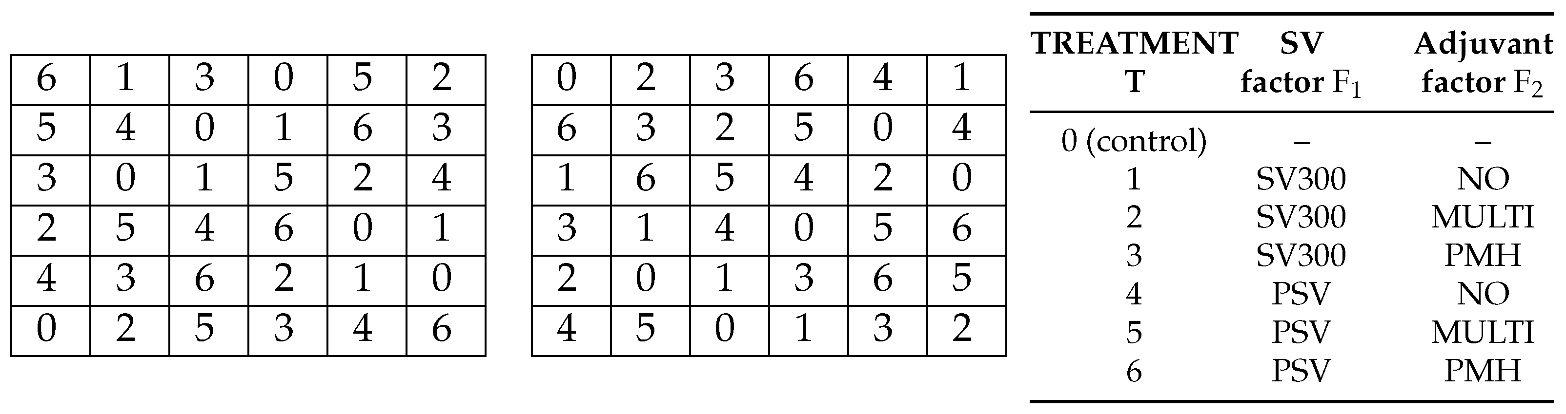
Therefore, the experiment investigated $v=7$ treatments: the control treatment and 6 experimental combinations of two spray systems (SV300 and PSV)–factor ${\mathrm{F}}_1$–and adjuvant additive (NO, MULTI or PMH)–factor ${\mathrm{F}}_2$. This type of arrangement gives a treatment structure called a near-factorial experiment [14,15]. Numerous construction methods for this type of experimental situation in the case of NRC designs are given by Bailey and Łacka [14] and Bose and Mukerjee [15], and it is from the first of these papers from which the plan for the distribution of treatments on experimental units comes—see Figure 3.

4.2. Statistical Analysis and Results

Based on the infestation results obtained in 2011, data were generated (

Table 2. Experimental data for a field experiment concerning the infestation of tomato plants by potato late blight (Phytophthora infestans (Mont.) De Bary). The experiment was carried out according to the scheme in Figure 3.

T	Block	RowNR	Col.NR	Obs.	T	Block	RowNR	Col.NR	Obs.
6	1	1	1	71.960	0	2	7	7	91.812
1	1	1	2	77.501	2	2	7	8	73.984
3	1	1	3	67.575	3	2	7	9	54.820
0	1	1	4	94.480	6	2	7	10	61.700
5	1	1	5	75.321	4	2	7	11	70.860
2	1	1	6	86.494	1	2	7	12	71.447
5	1	2	1	71.806	6	2	8	7	65.981
4	1	2	2	74.680	3	2	8	8	49.203
0	1	2	3	95.943	2	2	8	9	67.858
1	1	2	4	67.492	5	2	8	10	60.500
6	1	2	5	60.864	0	2	8	11	91.317
3	1	2	6	77.532	4	2	8	12	73.392
3	1	3	1	69.535	1	2	9	7	73.379
0	1	3	2	91.750	6	2	9	8	59.850
1	1	3	3	73.470	5	2	9	9	59.127
5	1	3	4	68.000	4	2	9	10	62.750
2	1	3	5	78.925	2	2	9	11	70.702
4	1	3	6	78.283	0	2	9	12	91.160
2	1	4	1	88.079	3	2	10	7	65.208
5	1	4	2	65.770	1	2	10	8	67.356
4	1	4	3	78.756	4	2	10	9	57.450
6	1	4	4	70.900	0	2	10	10	90.479
0	1	4	5	94.250	5	2	10	11	59.904
1	1	4	6	83.996	6	2	10	12	62.756
4	1	5	1	86.975	2	2	11	7	76.406
3	1	5	2	65.698	0	2	11	8	87.267
6	1	5	3	69.600	1	2	11	9	61.321
2	1	5	4	74.124	3	2	11	10	64.752
1	1	5	5	75.596	6	2	11	11	58.880
0	1	5	6	100.000	5	2	11	12	62.284
0	1	6	1	100.000	4	2	12	7	62.861
2	1	6	2	78.192	5	2	12	8	58.007
5	1	6	3	64.362	0	2	12	9	89.048
3	1	6	4	59.416	1	2	12	10	65.904
4	1	6	5	66.512	3	2	12	11	63.815
6	1	6	6	82.500	2	2	12	12	78.917

) and analyzed according to the methodology described in Section 3.2 (see Appendix A). The experimental field was divided into $b=2$ blocks with $c_0=r_0=6$ perpendicular rows and columns in each. The individual plot observations obtained for the combinations of the levels of factors ${\mathrm{F}}_1$ and ${\mathrm{F}}_2$ or the control treatment, taking into account their location in the rows and columns of each block, are shown in Table 2. Analyzing this experiment, we are interested in the verification of the general hypothesis (7) as well as determining the effectiveness of the applied protective procedures ($H_{0,\mathrm{C}}:{\mathit{U}}_{\mathrm{C}}^{\prime }{\mathbf{\tau }}_{*}=0$) and the significance of the main effects of the levels of factor ${\mathrm{F}}_1$ ($H_{0,{\mathrm{F}}_1}:{\mathit{U}}_{{\mathrm{F}}_1}^{\prime }{\mathbf{\tau }}_{*}=0$), the main effects of the levels of factor ${\mathrm{F}}_2$ ($H_{0,{\mathrm{F}}_2}:{\mathit{U}}_{{\mathrm{F}}_2}^{\prime }{\mathbf{\tau }}_{*}=0$), and the interaction effects of these two factors ($H_{0,{\mathrm{F}}_1{\mathrm{F}}_2}:{\mathit{U}}_{{\mathrm{F}}_1{\mathrm{F}}_2}^{\prime }{\mathbf{\tau }}_{*}=0$). These questions will be answered by estimating and testing certain sets of treatment parametric functions, which can be defined as follows:

$$\begin{array}{c}\hfill \left[\begin{array}{cc}0& 0_6^{\prime }\\ 0_6& {\displaystyle (}{\mathit{I}}_2-\frac{1}{2}{1}_2{1}_2^{\prime }{\displaystyle )}\otimes \frac{1}{3}{1}_3{1}_3^{\prime }\end{array}\right]\mathbf{\tau }={\mathit{U}}_{{\mathrm{F}}_1}^{\prime }\mathbf{\tau }\equiv {\mathit{U}}_{{\mathrm{F}}_1}^{\prime }{\mathbf{\tau }}_{*},\end{array}$$

$$\begin{array}{c}\hfill \left[\begin{array}{cc}0& 0_6^{\prime }\\ 0_6& \frac{1}{2}{1}_2{1}_2^{\prime }\otimes {\displaystyle (}{\mathit{I}}_3-\frac{1}{3}{1}_3{1}_3^{\prime }{\displaystyle )}\end{array}\right]\mathbf{\tau }={\mathit{U}}_{{\mathrm{F}}_2}^{\prime }\mathbf{\tau }\equiv {\mathit{U}}_{{\mathrm{F}}_2}^{\prime }{\mathbf{\tau }}_{*},\end{array}$$

$$\begin{array}{c}\hfill \left[\begin{array}{cc}0& 0_6^{\prime }\\ 0_6& {\displaystyle (}{\mathit{I}}_2-\frac{1}{2}{1}_2{1}_2^{\prime }{\displaystyle )}\otimes ({\mathit{I}}_3-\frac{1}{3}{1}_3{1}_3^{\prime })\end{array}\right]\mathbf{\tau }={\mathit{U}}_{{\mathrm{F}}_1{\mathrm{F}}_2}^{\prime }\mathbf{\tau }\equiv {\mathit{U}}_{{\mathrm{F}}_1{\mathrm{F}}_2}^{\prime }{\mathbf{\tau }}_{*},\end{array}$$

$$\begin{array}{c}\hfill \frac{\sqrt{10}}{6}\left[\begin{array}{cc}6& -1_6^{\prime }\end{array}\right]\mathbf{\tau }={\mathit{U}}_{\mathrm{C}}^{\prime }\mathbf{\tau }\equiv {\mathit{U}}_{\mathrm{C}}^{\prime }{\mathbf{\tau }}_{*},\end{array}$$

All these linear functions can be seen as contrasts of treatment parameters. For each of these four sets of contrasts, say ${\mathit{U}}_{\mathrm{L}},$ the BLUE is obtainable according to Formula (12), and the relevant sum of squares, $\mathrm{SS}({\mathit{U}}_{\mathrm{L}}),$ follows from (13). It can also be checked that

$$\begin{array}{c}\hfill \mathrm{SS}({\mathit{U}}_{\mathrm{C}})+\mathrm{SS}({\mathit{U}}_{{\mathrm{F}}_1})+\mathrm{SS}({\mathit{U}}_{{\mathrm{F}}_2})+\mathrm{SS}({\mathit{U}}_{{\mathrm{F}}_1{\mathrm{F}}_2})={\mathrm{SS}}_V,\end{array}$$

(15)

Now one can proceed to the general ANOVA (see Appendix A.1–Appendix A.3) and its partition into four components related to the sets of contrasts as in

Table 3. Analysis of variance for the sets of contrasts.

Source	Degrees of Freedom	Sum of Squares	Mean Square	$\hat{\mathit{F}}$	p Value
Treatments	6	450.024	75.004	75.004	<0.0001
${\mathrm{F}}_1$	1	14.3922	14.3922	14.3922	$0.00015$
${\mathrm{F}}_2$	2	35.9117	17.9558	17.9558	<0.0001
${\mathrm{F}}_1{\mathrm{F}}_2$	2	35.3518	17.6759	17.6759	<0.0001
C	1	364.368	364.368	364.368	<0.0001
Residuals	65	65	1
Total	71	515.0241

.

The critical values, at the 52.099 for 6 d.f., 3.841 for 1 d.f. and 2.996 for 2 d.f. The results presented in Table 3 were obtained with the use of the empirical estimates $\tilde{\mathbf{\tau }}$ and ${\tilde{\mathbf{\tau }}}_{*}$, i.e., based on ${\hat{\sigma }}_1^2=15.726$, ${\hat{\sigma }}_2^2=9.487$, ${\hat{\sigma }}_3^2=93.042$ and ${\hat{\sigma }}_4^2=1282.51$. The elements of vectors $\tilde{\mathbf{\tau }}$ and ${\tilde{\mathbf{\tau }}}_{*}$ are presented in

Table 4. Empirical estimates of $\mathbf{\tau }$ and ${\mathbf{\tau }}_{*}$. Treatments that do not differ significantly share a common letter.

TREATMENT	SV	Adjuvant	Treatment Effect	Main Effect
T	Factor ${\mathbf{F}}_1$	Factor ${\mathbf{F}}_2$	$\tilde{\mathit{\tau }}$	${\tilde{\mathit{\tau }}}_{*}$
0 (control)	–	–	93.125	(19.948)	a
1	SV300	NO	72.328	(−0.850)	c
2	SV300	MULTI	77.398	(4.221)	b
3	SV300	PMH	63.682	(−9.496)	d
4	PSV	NO	70.527	(−2.651)	c
5	PSV	MULTI	65.201	(−7.977)	d
6	PSV	PMH	65.993	(−7.185)	d

.

The estimates ${\hat{\sigma }}_i^2$ for $i=1,\dots ,4$ were obtained by solving Equation (8) using the iterative method (after five iteration steps, out of 20 performed, convergence was obtained) with the matrix ${\mathit{V}}_{*}^{-1}$ as suggested in Section 3.2.

The analysis of variance presented in Table 3 enabled rejection of the general hypothesis (7). The hypotheses concerning the factor ${\mathrm{F}}_1$, the factor ${\mathrm{F}}_2$ and their interaction were also rejected. The verification of the hypothesis $H_{0,\mathrm{C}}$ enabled determination of the effectiveness of the applied protective procedures. In this situation, the inference should be supplemented with detailed results, that is, a letter-based representation of all-pairwise comparisons (see Section 3.3). The contrasts used were normalized with respect to the treatment replication matrix, and the results are presented in Table 4.

5. Discussion and Conclusions

The high costs of conducting experiments should encourage the search for solutions enabling the effort put in to lead to success, understood by many researchers as the detection of significant differences between the studied treatments. When planning experiments, we make a number of decisions to solve the problems of which we are aware and those that we can only expect. These decisions will always influence the method of analyzing the results of the experiment. This paper recalls the principles that should be followed when planning an experiment. It is proposed to use a nested row–column design, which has wide practical application in agricultural experiments, and may be treated as an insurance policy against missed blocking. Thanks to the new, direct approach to the analysis of variance, inference for this type of experiment becomes simple and intuitive.

The methodology used here results from the use in the estimation and hypotheses testing procedures, of dispersion matrix not in the form

$$\begin{array}{c}\hfill \mathit{V}={\sigma }_1^2[{\mathbf{\varphi }}_1+({\sigma }_2^2/{\sigma }_1^2){\mathbf{\varphi }}_2+({\sigma }_3^2/{\sigma }_1^2){\mathbf{\varphi }}_3+({\sigma }_4^2/{\sigma }_1^2){\mathbf{\varphi }}_4+({\sigma }_5^2/{\sigma }_1^2){\mathbf{\varphi }}_5]={\sigma }_1^{2}F,\end{array}$$

usually applied in the literature, as Kala [25] mentions, but in its original form (3) which ensures that $\mathrm{E}({\mathrm{SS}}_R)=n-v$.

Another feature of the proposed approach concerns the simplification of the analytical procedures. One of the resulting advantages is the reduction of the number of stratum variances involved from 5 to 4. This widely simplifies the computations.

As Kala [25] notes, Equation (8) coincide-as it was observed by Patterson and Thompson [40]—with the equations following from their maximum likelihood approach under the assumption that $\mathit{y}$ has a multivariate normal distribution, with such an advantage, that here iteration is distribution free as it uses only geometrical arguments. The proposed approach ignores within-stratum analyses based on the stratum submodels and involved combined analysis. It is shown how to perform the analysis also in the case of factorial and near-factorial structures of treatments. The main advantage of the proposed approach is that the ANOVA results can be obtained directly rather than by first performing stratum analyses and then combining their results, as in the classic approach [23,24].

As shown in the publications [10,11,12,13] and presented in Table 1, the proposed procedures lead to the reduction of the residual sum of squares to $n-v$, which in turn leads to the form of the F statistic expressed by the Formula (10). This can be seen as an advantage for the approximation of the relevant distribution.

In the applicative approach, the estimated mean square has (under $H_0$) approximately the distribution of ${\chi }^2(v-1,0)/(v1)$. The greater is n, i.e., the size of the experiment, the closer this approximation will be. Thus, the test of hypothesis $H_0$ and the relevant critical level of significance are regarded as approximate. These conclusions correspond to those presented by Volaufova [41] and Johnson et al. [42].

The paper shows how to obtain a letter-based representation of all-pairwise comparisons using simple contrasts. The letter display, by far the most popular method for reporting the result of mean comparisons in all areas of research where ANOVA procedures are used, is now available after the analysis of variance under a derived mixed model in an NRC design is performed directly. All of this gives a complete set of tools that make it easy to analyze any NRC experiment. Appendix A provides all the necessary tools in R [43], and the example of a field experiment shows how the proposed procedure is performed in practice. An example of the data including a file structure compliant with the R code (Appendix A) is available in Table S1 in Supplementary Materials.

Finally, this approach can be applied to various classes of designs with the OBS property, in particular those shown in

Table 5. Parameters and models of experimental designs obtained if certain block structures of the NRC design are omitted. The starting point is the design shown in Figure 2. The omitted block structures correspond to the deleted elements of the base model (1).

ROW-COLUMN DESIGN ($\mathit{b}=\mathbf{1}$)
Parameters
Model
	$\mathit{V}={\sigma }_1^2{\mathbf{\varphi }}_1+{\sigma }_2^2{\mathbf{\varphi }}_2+{\sigma }_3^2{\mathbf{\varphi }}_3+{\sigma }_5^2{\mathbf{\varphi }}_5$ taking ${\mathit{X}}_B=1_n$
	${\mathit{V}}_{*}={\sigma }_1^2({\mathbf{\varphi }}_1-{\mathbf{\varphi }}_5)+{\sigma }_2^2({\mathbf{\varphi }}_2+{\mathbf{\varphi }}_5)+{\sigma }_3^2({\mathbf{\varphi }}_3+{\mathbf{\varphi }}_5)$
NESTED BLOCK DESIGN
Parameters
Model
	$\mathit{V}={\sigma }_1^2{\mathbf{\varphi }}_1+{\sigma }_2^2{\mathbf{\varphi }}_2+{\sigma }_4^2{\mathbf{\varphi }}_4+{\sigma }_5^2{\mathbf{\varphi }}_5$ taking ${\mathbf{\varphi }}_1={\mathit{I}}_n-c_0^{-1}{\mathit{X}}_{R(B)}{\mathit{X}}_{R(B)}^{\prime }$
	${\mathit{V}}_{*}={\sigma }_1^2{\mathbf{\varphi }}_1+{\sigma }_2^2{\mathbf{\varphi }}_2+{\sigma }_4^2({\mathit{I}}_n-{\mathbf{\varphi }}_1-{\mathbf{\varphi }}_2)$
PROPER BLOCK DESIGN
Parameters
Model
	$\mathit{V}={\sigma }_1^2{\mathbf{\varphi }}_1+{\sigma }_4^2{\mathbf{\varphi }}_4+{\sigma }_5^2{\mathbf{\varphi }}_5$ taking ${\mathbf{\varphi }}_1={\mathit{I}}_n-n_0^{-1}{\mathit{X}}_B{\mathit{X}}_B^{\prime }$
	${\mathit{V}}_{*}={\sigma }_1^2{\mathbf{\varphi }}_1+{\sigma }_4^2({\mathit{I}}_n-{\mathbf{\varphi }}_1)$

.

As previously noted, sometimes it turns out following an experiment that the applied approach needs to be reviewed. If the estimated row- (or column-) related variance components are small, close to zero, then the analysis reverts to the model for a simpler block structure—a nested block design. If both the row and column variances are close to zero, then the experiment should be run as for a proper block design [8]. Finally, if the researcher has data only from one block, the analysis will follow the model for a row–column design.

Since the starting point for the analysis is the NRC design, each of the possible modified analyses will be carried out for a design with an orthogonal block structure, which makes it possible to apply the direct approach [10,11,12,13]. As the practical application of this analytical approach depends on the structure of the experimental design, Table 5 shows how the model of the NRC design will change when some block structures are omitted. Of course, for new designs, the structure of the dispersion matrix $\mathit{V}$ changes and therefore a different matrix ${\mathit{V}}_{*}$ should be used for each of them. Next, the analytical procedure will be analogous to that in Section 3.2. The notation used in Table 5 is based on the notation of the output NRC design, so only some of the ${\sigma }_i^2{\mathbf{\varphi }}_i$ components appear in the matrix $\mathit{V}$. It should be noted here that since the roles of rows and columns in the NRC design can be changed, the nested block design is presented only for the case of the omission of the NRC’s column system. Usually the system we call “blocks” (by analogy with the NRC design) is called “superblocks” for a nested block design, while our “rows” are called “blocks”.

References

- Fisher, R.A. Statistical Methods for Research Workers, 11th ed. rev.; Oliver and Boyd: Edinburgh, UK, 1925. [Google Scholar]
- Fisher, R.A. The arrangement of field experiments. J. Minist. Agric. 1926, 33, 503–515. [Google Scholar]
- Yates, F. A fresh look at the basic principles of the design and analysis of experiments. In Proceedings of the Fifth Berkeley Symposium on Mathematical Statistics and Probability, Statistical Laboratory, University of California, Berkeley, CA, USA, 21 June–18 July 1965 and 27 December 1965–7 January 1966; University of California Press: Berkeley, CA, USA, 1967; pp. 777–790. [Google Scholar]
- Hinkelmann, K.; Kempthorne, O. Design and Analysis of Experiments. Vol. 1. Introduction to Experimental Design, 2nd ed.; Wiley-Interscience: New York, NY, USA, 2008. [Google Scholar]
- Casler, M.D. Fundamentals of Experimental Design: Guidelines for Designing Successful Experiments. Agron. J. 2015, 107, 692–705. [Google Scholar] [CrossRef] [Green Version]
- LeClerg, E.L.; Leonard, W.H.; Clark, A.G. Field Plot Technique, 2nd ed.; Burgess Publishing Company: Minneapolis, MN, USA, 1966. [Google Scholar]
- Grzebisz, W.; Łukowiak, R. Nitrogen Gap Amelioration Is a Core for Sustainable Intensification of Agriculture—A Concept. Agronomy 2021, 11, 419. [Google Scholar] [CrossRef]
- Bailey, R.A.; Williams, E.R. Optimal nested row-column designs with specified components. Biometrika 2007, 94, 459–468. [Google Scholar] [CrossRef]
- Caliński, T.; Kageyama, S. Block Designs: A Randomization Approach, Vol. I: Analysis; Lecture Notes in Statistics (Volume 150); Springer: New York, NY, USA, 2000; pp. 154–196. [Google Scholar]
- Caliński, T.; Siatkowski, I. On a new approach to the analysis of variance for experiments with orthogonal block structure. I. Experiments in proper block designs. Biom. Lett. 2017, 54, 91–122. [Google Scholar] [CrossRef] [Green Version]
- Caliński, T.; Siatkowski, I. On a new approach to the analysis of variance for experiments with orthogonal block structure. II. Experiments in nested block designs. Biom. Lett. 2018, 55, 147–178. [Google Scholar] [CrossRef] [Green Version]
- Caliński, T.; Łacka, A.; Siatkowski, I. On a new approach to the analysis of variance for experiments with orthogonal block structure. III. Experiments in row-column designs. Biom. Lett. 2019, 56, 183–213. [Google Scholar] [CrossRef] [Green Version]
- Caliński, T.; Łacka, A.; Siatkowski, I. On a new approach to the analysis of variance for experiments with orthogonal block structure. IV. Experiments in split-plot designs. Biom. Lett. 2020, 57, 183–213. [Google Scholar] [CrossRef]
- Bailey, R.A.; Łacka, A. Nested row-column designs for near-factorial experiments with two treatment factors and one control treatment. J. Stat. Plan. Inference 2015, 165, 63–77. [Google Scholar] [CrossRef] [Green Version]
- Bose, M.; Mukerjee, R. Near-factorial experiments in nested row-column designs regulating efficiencies. J. Stat. Plan. Inference 2017, 193, 109–116. [Google Scholar] [CrossRef]
- Gupta, S.; Kageyama, S. TypeS designs with nested rows and columns. Metrika 1991, 38, 195–202. [Google Scholar] [CrossRef]
- Hartung, J.; Wagener, J.; Reiner, R.; Piepho, H.-P. Blocking and re-arrangement of pots in greenhouse experiments: Which approach is more effective? Plant Methods 2019, 15, 143. [Google Scholar] [CrossRef] [Green Version]
- Kozłowska, M.; Łacka, A.; Skorupska, A. Block designs with nested rows and columns for research on food acceptability limitation. Commun. Stat. A-Theory 2012, 41, 2456–2464. [Google Scholar] [CrossRef]
- Chang, J.Y.; Notz, W.I. Some optimal nested row-column designs. Stat. Sin. 1994, 4, 249–263. [Google Scholar]
- Łacka, A.; Kozłowska, M. Planning of factorial experiments in a block design with nested rows and columns for environmental research. Environmetrics 2009, 20, 730–742. [Google Scholar] [CrossRef]
- Pearce, S. The factorial field experiment. Exp. Agric. 2005, 41, 109–120. [Google Scholar] [CrossRef]
- Caliński, T.; Łacka, A. On Combining Information in Generally Balanced Nested Block Designs. Commun. Stat. A-Theory 2014, 43, 954–974. [Google Scholar] [CrossRef]
- Yates, F. The recovery of inter-block information in variety trials arrangedin three-dimensional lattices. Ann. Eugen. 1939, 9, 136–156. [Google Scholar] [CrossRef]
- Yates, F. The recovery of inter-block information in balanced incompleteblock designs. Ann. Eugen. 1940, 10, 317–325. [Google Scholar] [CrossRef]
- Kala, R. A new look at combining information from stratum submodels. In Matrices, Statistics and Big Data, Selected Contributions from IWMS 2016; Ahmed, S.E., Carvalho, F., Puntanen, S., Eds.; Springer: Berlin/Heidelberg, Germany, 2019; pp. 35–49. [Google Scholar]
- Singh, M.; Dey, A. Block designs with nested rows and columns. Biometrika 1979, 66, 321–326. [Google Scholar] [CrossRef]
- Nelder, J.A. The analysis of randomized experiments with orthogonal block structure. Proc. R. Soc. Lond. A 1965, 283, 147–178. [Google Scholar]
- Kozłowska, M.; Łacka, A.; Krawczyk, R.; Kozłowski, R.J. Some block designs with nested rows and columns for research on pesticide dose limitation. Environmetrics 2011, 22, 781–788. [Google Scholar] [CrossRef]
- Mejza, I.; Mejza, S. Model Building and Analysis for Block designs with Nested Rows and Columns. Biom. J. 1994, 36, 327–340. [Google Scholar] [CrossRef]
- Houtman, A.M.; Speed, T.P. Balance in designed experiments with orthogonal block structure. Ann. Stat. 1983, 11, 1069–1085. [Google Scholar] [CrossRef]
- Rao, C.R.; Kleffe, J. Estimation of Variance Components and Applications; North-Holland: Amsterdam, The Netherlands, 1988. [Google Scholar]
- Rao, C.R. Projectors, generalized inverses and the BLUEs. J. R. Stat. Soc. Ser. B 1974, 36, 442–448. [Google Scholar]
- Nelder, J.A. The combination of information in generally balanced designs. J. R. Stat. Soc. Ser. B 1968, 30, 303–311. [Google Scholar] [CrossRef]
- Piepho, H.-P. An Algorithm for a Letter-Based Representation of All-Pairwise Comparisons. J. Comput. Graph. Stat. 2004, 13, 456–466. [Google Scholar] [CrossRef]
- Graves, S.; Piepho, H.-P.; Selzer, L. With Help from Dorai-Raj S. multcompView: Visualizations of Paired Comparisons. R Package Version 0.1-8. 2019. Available online: https://CRAN.R-project.org/package=multcompView (accessed on 19 December 2019).
- Lenth, R.V. Least-Squares Means: The R Package lsmeans. J. Stat. Softw. 2016, 69, 1–33. [Google Scholar] [CrossRef] [Green Version]
- Ratajkiewicz, H.; Kierzek, R.; Raczkowski, M.; Hołodyńska-Kulas, A.; Łacka, A.; Szulc, T. The effect of coarse-droplet spraying with double flat fan air induction nozzle and spray volume adjustment model on the efficiency of fungicides and residues in processing tomato. Span. J. Agric. Res. 2018, 16, e1001. [Google Scholar] [CrossRef]
- Ratajkiewicz, H.; Kierzek, R.; Raczkowski, M.; Hołodyńska-Kulas, A.; Łacka, A.; Wójtowicz, A.; Wachowiak, M. Effect of the spray volume adjustment model on the efficiency of fungicides and residues in processing tomato. Span. J. Agric. Res. 2016, 14, e1007. [Google Scholar] [CrossRef] [Green Version]
- Bailey, R.A. Hasse diagrams as a visual aid for linear models and analysis of variance. Commun. Stat. A-Theory 2020, 50, 5034–5067. [Google Scholar] [CrossRef]
- Patterson, H.D.; Thompson, R. Recovery of inter-block information when the block sizes are unequal. Biometrika 1971, 58, 545–554. [Google Scholar] [CrossRef]
- Volaufova, J. Heteroscedastic ANOVA: Old p values, new views. Stat. Pap. 2009, 50, 943–962. [Google Scholar] [CrossRef]
- Johnson, N.L.; Kotz, S.; Balakrishnan, N. Continuous Univariate Distributions, 2nd ed.; Wiley: New York, NY, USA, 1995; Volume 2. [Google Scholar]
- R Core Team. R: A Language and Environment for Statistical Computing; R Foundation for Statistical Computing: Vienna, Austria, 2020; Available online: https://www.R-project.org/ (accessed on 15 February 2021).
- Bates, D.; Maechler, M. Matrix: Sparse and Dense Matrix Classes and Methods. R Package Version 1.3-4. 2021. Available online: https://CRAN.R-project.org/package=Matrix (accessed on 1 June 2021).
- Coelho, G.; Mation, L. utilsIPEA: IPEA Common Functions. R Package Version 0.0.6. 2018. Available online: https://CRAN.R-project.org/package=utilsIPEA (accessed on 20 April 2018).
- Friendly, M.; Fox, J.; Chalmers, P. matlib: Matrix Functions for Teaching and Learning Linear Algebra and Multivariate Statistics. R Package Version 0.9.4. 2020. Available online: https://CRAN.R-project.org/package=matlib (accessed on 25 October 2020).
- Revelle, W. psych: Procedures for Personality and Psychological Research; Northwestern University: Evanston, IL, USA, 2021; Available online: https://CRAN.R-project.org/package=psychVersion=2.1.6. (accessed on 20 June 2021).
Figure 1.
Casler’s [5] flow diagram of the logical steps in scientific experimentation, including a feedback loop that allows for new scientific hypotheses and experimental design modifications to future experiments. The three central boxes form the “statistical triangle” [4].
Figure 2.
Schematic diagram of a nested row–column design with b blocks (here ), each grouped perpendicularly into rows of units and columns of units.
Figure 3.
Scheme of distribution of treatments 0–6 on experimental units of the NRC design with blocks. Each block has rows and columns. The number at the intersection of a row and column indicates the treatment used in that plot. Treatment numbers are consistent with the legend on the right side of the diagram.