Characteristic Decrease in the Value of Rapeseed Evapotranspiration after Its Ripening

Abstract

This paper presents the methodology of taking measurements of active surface energy balance components using the Bowen method. It discusses the applied measurement system, an important part of which are HMD 50U/50Y measurement sensors from Vaisala, adapted to work in the field. Their operation is a source of data for determining vertical profiles of temperature and water vapour pressure. These data are used to determine the turbulence components of the energy balance, i.e., sensible and latent heat. Measurements taken during the vegetative season on rape field showed that intensive evaporation occurred in the period until the end of June and that its decrease coincided with the decrease in the value of the degree of plant development determined on the basis of LAI records. In spring, during the period of intensive plant development, the decade sums of evaporation reached 30 mm, after which their quantities fell to the range of 10–15 mm. They became higher only in the periods of precipitation, when the water from the interception was available.

1. Introduction

Human development over the last several hundred years has had a strong impact on environmental changes, with agriculture leading to huge area changes. Gradual population growth forced the allocation of more and more areas for agricultural production, and then, this growth intensified, necessitating increased production to provide access to food. This, however, entailed an increasing burden on the environment. Not only did agriculture occupy vast areas of land, it also had a highly invasive effect on other environmental components. In addition, globalization, i.e., the increase of integration in internationally dispersed activities, influences agriculture, people’s living environment, and the use of resources [1,2,3,4].

Rape is one of the most-grown plants, with worldwide crops of around 65–70 million tons. It is mainly used for the production of cooking oil, but it is also a source of biofuel. If its use as a fuel becomes popular, the acreage of its cultivation will significantly increase. Rapeseed is a winter crop, so it uses both the autumn and spring vegetation period, but it matures and dries up relatively quickly, which means that the field is often devoid of vegetation during the summer. It is very unfavourable from the point of view of the environment and agriculture. Hence, it was decided to follow the shaping of the components of the heat balance, including the evapotranspiration of rape during the growing season.

2. Active Surface Energy Balance

Generally, in the literature, active surface is understood as a plane through which the flow of energy and matter fluxes occurs, during which the transformation of individual fluxes often takes place. It is assumed to have zero thermal capacity and mass, so the energy balance of a surface is given in the following Equation (1) [5,6,7,8,9,10].

$$Rn+LE+H+G=0$$

(1)

where: Rn—net radiation [W·m⁻²],

• LE—latent heat flux density [W·m⁻²],
• H—sensible heat flux density [W·m⁻²],
• G—soil heat flux density [W·m⁻²].

The energy and mass exchange in the atmosphere layer above the active surface takes place in a turbulent manner [7,8,11,12,13,14,15]. One of the ways to determine vertical mass and energy fluxes is to use independent measurements of the net radiation and the soil flux as well as data on the temperature and water vapour pressure profile, in the so-called Bowen ratio energy balance method. The ratio of sensible heat flux density to latent heat (2) was assumed to be called Bowen ratio (β), as he was the first [16] to compare the heat flux used for heating the air with the flux used for water evaporation:

$$\beta =\frac{S}{LE}$$

(2)

Applying to this equation formulas for the estimation of sensible (S) and latent (LE) heat resulting from the profile method, described in the above-mentioned literature, leads to the following result:

$$\beta \left(z\right)=\gamma ·\frac{\frac{dt\left(z\right)}{dz}}{\frac{de\left(z\right)}{dz}}$$

(3)

where:

• e(z)—water vapour pressure at the height of (z) [hPa],
• t(z)—air temperature at the height of (z) [°C],
• γ—psychrometric constant = 0.66 hPa K⁻¹.

Using the active surface energy balance equation and Bowen ratio, it is possible to determine the turbulence values of energy balance components. This procedure is called Bowen ratio energy balance method. This method was used in field studies, the results of which were applied in this work.

Using the Bowen ratio energy balance method, the equality of the turbulent transport coefficients for water vapor and sensible heat were assumed. The correctness of such a solution is supported by the fact that the measurements were made in a square-shaped field of approx. 70 ha, so there were distances of more than 300 m from the edge of the field to the measuring mast. Then it can be expected that almost always the measurement was carried out in the developed boundary layer. In addition, the surrounding fields were also farmed, meaning that advective heat flows were unlikely. Calculations during the measurements showed that the vertical profiles of water vapor temperature and pressure were generally consistent (for example as in Figure 3), which also confirms the above.

In the publication of Irmak et al. [17] it was shown that the turbulence exchange coefficient of water vapor is on average higher than the sensible heat, but the Eddy covariance method was used for verification, which also has some limitations. Moreover, it seems important that the measurements were made on the cultivation of subsurface irrigated maize, which meant that the main or perhaps the only source of water vapor were evapotranspirating plants without the soil surface, which in the case of tall plants could intensify this process, but it is debatable.

The Bowen method of ratio energy balance evaluation is one of the ways in which the agricultural crops water consumption is estimated and is often used to evaluate models that estimate these quantities [17,18,19,20,21,22,23,24,25]. In the case of very high plant transpiration capacity, which occurs with well-developed plant cover and water availability in the soil, most of the energy from the radiation balance is used for latent heat. In the event of limitations due to access to water or poor condition of the plant cover, this energy is used to heat the soil and air [26,27]. The problem arises here in how to determine the condition of plants in the most measurable way possible. Olejnik [28] proposed to take into consideration the height of plants, but this parameter would have to be determined separately for each species or a variety of cultivated plants (habitat type). A more universal parameter is the Leaf Area Index (LAI), which was measured on the studied plot. It reflects the surface area of leaves which play a decisive role in the interception quantity and in the absorption of solar radiation [29,30,31].

The literature also gives examples of using the leaf area index in agricultural practice to determine the state of vegetation, to forecast yields, to plan planting density, and in forest management to estimate forests’ net production or as an indicator of leaf damage caused by freezing rain and hail [32,33,34,35,36]. LAI is also one of the basic input data of many models, with different scales (from micro to global), used to analyse not only the aforementioned, but also many other processes [37,38].

3. Research Area

The measurements, the results of which were used in this work, were taken on the farmland located near the village of Chlewiska with coordinates: 52°30′ N and 17°39′ E.

For the selected research area, the average annual air temperature from multiannual period of 1971–2000 is 8.2 °C [39]. The average annual sum of corrected precipitation (P) for the area of Poznań is 605 mm, and actual evapotranspiration (ETR) 469 mm [40], the vegetation period lasts 226 days on average, the average total annual cloud cover is 65%, water vapour pressure is 9.2 hPa, and relative humidity about 78% [39].

4. Research Methodology

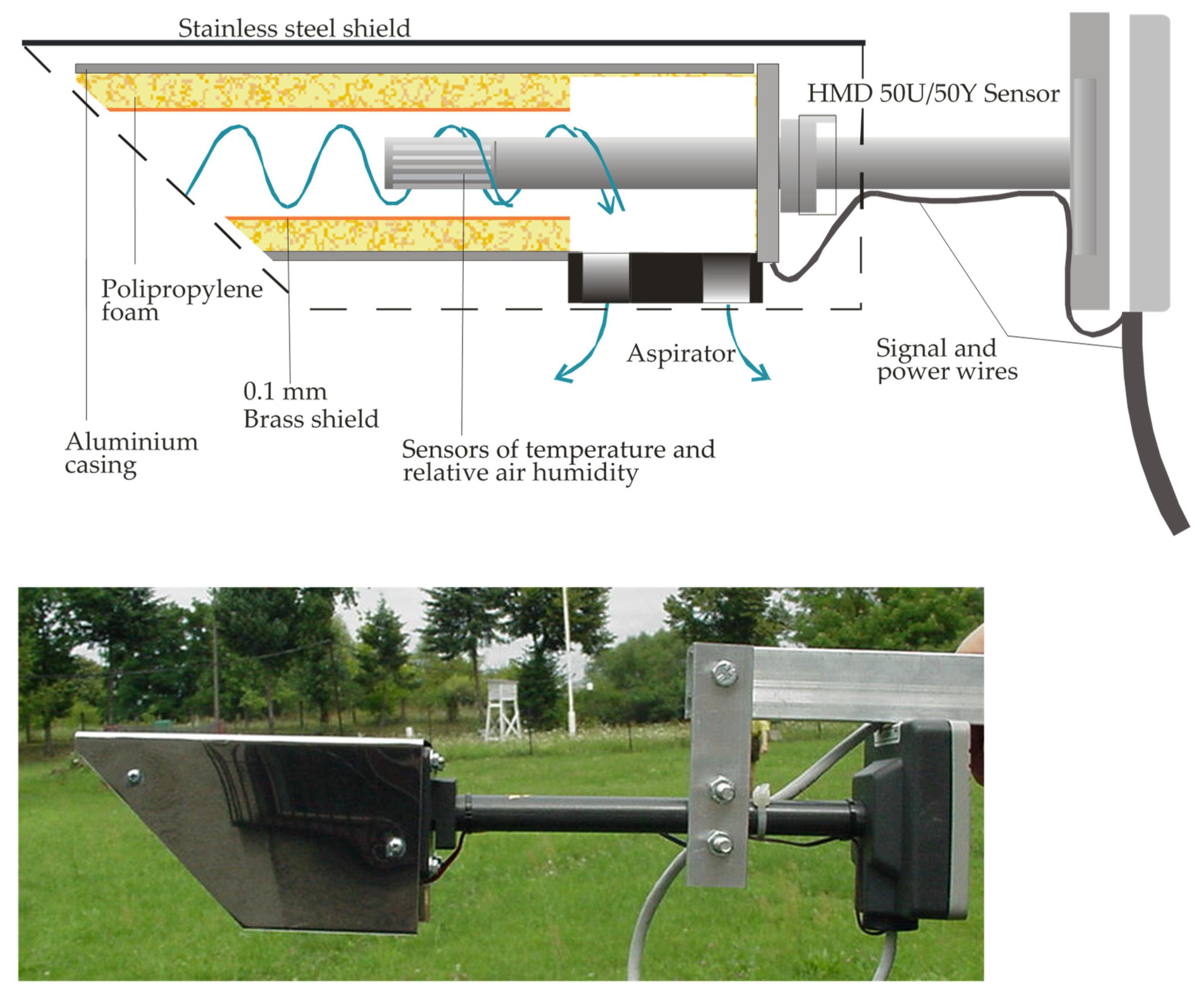
Vaisala HMD 50U/50Y sensors were used for vertical measurements of temperature and water vapour pressure profiles in the air, among which the INTERCAP^® no. 15778HM sensor is used to measure relative humidity and PT1000 IEC 751 class B to measure temperature (Vaisala, Finland). During the measurements, an output signal in the 0–1 V range was used for the humidity sensor; the only available output signal for temperature in the 0–10 V range was processed by means of a system of highly temperature-stable resistors into a signal in the 0–1 V range. Before using the sensors in the research, their additional testing was carried out in a special calibration chamber [41].

The described sensors required designing a special casing with several insulation layers, according to the diagram in Figure 1. The casing protected the sensors from the radiation of the environment by enclosing them in a shield consisting of thin-walled brass sheet (0.1 mm), a layer of thermo-insulating foam, an aluminium casing and a mantle made of stainless steel. Thanks to its high albedo (mirror-like gloss), the shield reflected solar radiation and at the same time protected all sensor elements from rain and additionally fulfilled a constructional role (Figure 1). A fan with a power of merely 0.6 W was used for ventilation, which did not significantly increase the amount of energy required.

In the measuring system used for the research in 2002 to measure radial energy, a pyrgeometer was used in combination with a CNR1 Kipp-Zonnen pyranopyrgeometer (measurements over rapeseed and then over stubble and over the plowed field, Figure 2) (Kipp & Zonen Delft, The Netherlands).

Hukseflux soil tiles were used to measure soil heat flux (Hukseflux Thermal Sensors B.V. Delft, The Netherlands).

KEST data logger with 32 measurement channels was used to record the data (KEST ELECTRONICS, Poznań, Poland). The data are stored there on removable FLASH memory cards. The data logger also has a special control channel which triggers the aspiration of psychrometers in the system. The measurement at each channel takes $\frac{1}{3}s$. Measurements are performed successively at all channels and merge into measurement cycles, which can be repeated no more often than every 20 s. They can be combined into measurement series consisting of any number of cycles, or they can be performed continuously—this is how it was done in the case of the described measurements.

5. Methodology for Calculating the Active Surface Energy Balance Components

As it has already been mentioned, measurements of such parameters as temperature vertical profiles, water vapour pressure, radiation balance and heat flux balance exchanged with the soil were performed around the clock. The results obtained were then used to determine the components of the active surface energy balance. All calculations were conducted using Visual Basic procedures, which allow for much more complex calculations than standard spreadsheet tools.

On the basis of temperature and relative humidity, water vapour pressure quantities were determined and then the hourly averages were calculated at each measurement level. In turn, these mean values of temperature and water vapour pressure lay basis for approximating functions t(z) and e(z) describing water vapour pressure and temperature changes over the active surface.

From the literature [7], and from experience, we conclude that the best approximation for vertical variability, as for wind speed, is obtained using the following logarithmic Function (4):

$$t\left(z\right)=a_t·ln\left(z-D_h\right)+b_t$$

(4)

where: z—height above the ground, $a_t, b_t, D_h$—parameters determined by the least squares method. $D_h$ was determined for air temperature and it was assumed that it would take the same value for water vapour pressure. This parameter shows the asymptote of functions describing variability with temperature value and water pressure quantity and they can be equated with zero plane displacement. It usually takes values from 0 to the height of the lowest sensor located above the plant cover. However, it should be pointed out here that the determined functions satisfactorily describe changes in the parameters only in a small turbulence layer above the plants, where they change logarithmically. In the vegetation this variability is disturbed hence the above remark. The presented procedure was applied for each hour of measurements. Each time the quality of the adjustment of the approximated functions was evaluated by means of a determination factor and it was checked whether they were within the range of confidence intervals for the recorded average values.

Figure 3 shows the approximation of the vertical variability of temperature and pressure of water vapour for the average values of 180 measurements on each level taken from 1100 to 1200 on 22 May. Figure 3 shows only averages and their 95% confidence intervals. Initially, the trend was eliminated from the measurement data and due to fluctuations of values resulting from turbulent air movement, the data were smoothed to 5-min periods (a moving average from 15 observations). The determination factor (R2) calculated for all measurements ($n=800$) was 0.53 for temperature approximation and 0.68 for water vapour pressure approximation respectively.

Using the equations of the profile method of turbulence fluxes evaluation described above, the value of Bowen ratio at z height can be given according to the Formula (3).

In the given example of 22 May, Bowen ratio was 0.27.

Using Equations (1) and (3), one can now calculate the energy fluxes used for evaporation (LE) and the energy used for air heating (S).

As a standard, the Bowen method uses a gradients quotient, i.e., the values of temperature and water vapor pressure are measured on two levels, then the gradients and their quotient are calculated. This always raises the question of whether the sensors are at the correct height and whether their accuracy is good enough. In the method used, functions describing the vertical variability of temperature and steam pressure are determined, which allows to determine point gradients at any height and their ratio, thus eliminating the above-mentioned question about the correct height of the sensor arrangement.

Bowen method requires the measuring mast to be placed over a sufficiently large area covered by homogeneous vegetation so that the boundary layer characteristic for the area can develop properly. Therefore, the measurements of the thermal balance components, which started on 24 April, as already mentioned in point 2, were made on a 70 ha field. The measuring mast was placed in the centre of the field, so that regardless of the wind direction, the boundary layer characteristic for the given area could develop.

6. The Meteorological Conditions during the Course of Research

Figure 4 presents the average ten-day temperature courses from the station in Poznań and from the field measurements in Chlewiska in 2002, against the average values from the multiannual period of 1971–2000. The average temperature in 2002 was 10.0 °C, which was 1.2 °C degrees higher than the average from 1973–2003, i.e., 8.8 °C. Comparing the multi annual values with the decade averages of 2002, it can be seen that the beginning of the vegetation period (March, April) did not differ significantly from the averages. Both decades of warmer and cooler than average values occurred during that period. In turn, during the research period, that is from May to September, almost all decades were warmer than average. The beginning of May and the end of August were the warmest in relation to the averages, only the end of September was cooler.

However, these values do not indicate that 2002 was exceptionally warm, but rather fit into the climate warming trend. It is also worth noting that the temperature recorded in the field was lower than that from the station in Poznań.

Figure 5 presents the annual course of average monthly precipitation sums from the stations in Poznań and Szamotuły (the nearest Chlewiska stations in the Institute of Meteorology and Water Economy Network) from 1971 to 2000 [39] and monthly sums of precipitation on fields in Chlewiska in 2002. In terms of precipitation, from May to September the year 2002 was rather dry. Average sums of precipitation in these months range from 315 mm in Poznan to 323 mm in Szamotuły [39], while in 2002 only 205 mm of precipitation was recorded in Chlewiska. At the same time the precipitation measured in May and August was even slightly above the average, while much less than the average was recorded in June and July. In both months it fell below 30 mm and it was less than 50 averages from multiannual period. Such low rainfall had a very noticeable effect on soil moisture and consequently on plants accessibility to water, which in turn resulted in a decrease in evapo-transpiration.

7. Results and Discussion

Figure 6 presents the seasonal pattern of decade precipitation and evaporation quantities. Evaporation quantities were determined on the basis of recorded energy fluxes used for evapotranspiration, using the mass of evaporated water equivalent with the energy required for this process.

Comparing the recorded quantities of actual precipitation in the vegetation season of 2002 with the average sums from multiannual period, it can be concluded that 2002 was a year with a relatively low precipitation. The total recorded precipitation from the beginning of April to the end of September that year was 287 mm (205 mm from May to September), while the average multi-annual sum was 359 mm. The resulting difference is mainly due to the long period of very low rainfall that occurred in June and July 2002. During those months, the last relatively high rainfall of 9.6 mm was recorded on 7 June from that moment until 4 August, the highest recorded rainfall was only 4.6 mm (14 July). In total, during that period (58 days), only 39 mm of rain fell, which covers only about a fifth of the water that some crops can vaporize during such period. Therefore, if we count the evaporation and rainfall cumulatively from 8 June to 4 August, for some crops, the water deficiency would reach 160 mm. Such a large water deficit would be only in crops that were in full physiological activity during that period: beets, potatoes or grassland. Therefore, the evaporation, which was recorded at that time, was largely occurring due to moisture reserves in the soil. This is natural for this time of the year, but generally the deficit is smaller. The analysis of the monthly accumulated rainfall shows that the rainfall recorded in June was 39 mm and represented only 56% of the multiannual average for that month. July, which is usually the month with the highest total annual precipitation, was characterized by 35 mm of precipitation, which was only 45% of the multiannual average. In the remaining months, the precipitation did not differ significantly from the multiannual averages.

For the cultivation of oilseed rape (Figure 6), in order to maintain the proportions of the figures for the months in which the III decade had 11 days, the quantity of the measured sum was multiplied by 10/11), the evapotranspiration of the III decade of April was determined proportionally on the basis of the results from the last four days of April, and the I decade of October on the basis of one day of measurements only)

The course of the decade-long evaporation quantities very clearly coincides with plant development. If we consider daily evaporation rates, their variability is greatly affected by the weather. During the decade there are days with sunny weather and high evaporation, as well as rainy days with very little one, so the sum of evaporation reflects mainly physiological activity of plants. It should be noted, however, that over longer periods of time this activity is also related to the availability of water and in the case of water depletion in the soil, e.g., due to low rainfall, it may gradually decrease. On rape field, high evaporation was recorded in May and June, i.e., first when the plants were still growing very intensively and then when the seeds were formed. The decrease of evapotranspiration was observed already in the last decade of June, when the plants started to dry out. In the field studied rape was mown on 12 July, when the plants were obviously already completely dry. This was clearly reflected in the very small evaporation quantity in the first decade of July, and was no different from the evaporation in the decades after the harvest. Additionally, the low evaporation in July was a result of low rainfall quantities both in June and July. On the other hand, intensive evaporation in the second and third decade of August is a result of two elements: frequent precipitation and gradual overgrowth of the stubble.

As it has been mentioned, the described evaporation cannot be separated from the development of plants, whose measurable parameter is the leaf area index (LAI). The device LAI-2000 (LaiCor) was used to measure it. Phenology uses the concept of developmental phase which is a descriptive concept and refers to the so-called appearances, e.g., plant emergence and onset of flowering. Following the development of crops, especially cereals and rape, it can be seen that the individual phases of development are related to the height of plants and their LAI. Originally in the literature, in order to parametrize the development of plants, the conceptual treatment of the developmental phase was abandoned and replaced by a numerical value expressing the ratio of the current height of plants to their maximum height during the entire vegetation period [7,8,13,28,38]. Such determination of the developmental phase resulted in its relatively late increase and a long-lasting value equal to one, from the moment of reaching the maximum height to the time of mowing the plants.

Analysing the course of the recorded LAI values, it can be observed that the development of plants occurred faster than originally reported in the cited literature, the maximum leaf area index occurred about two 10-day periods earlier than the full development of plants (maximum height), according to the mentioned publications. This indicates excessive time extension of the estimated phase at the stage of intensive plant growth, resulting from the above-mentioned method of determining the developmental phase value.

It is possible that the maximum LAI value will be reached earlier than the maximum height, because while the plants are still growing, the leaves from the winter period and those that appeared the earliest are already beginning to die, so it is possible that the height can increase without the growth of LAI, and in extreme cases even with its decrease.

Another important difference is the already mentioned length of the period in which the plants are at the developmental phase that equals one (maximum). Taking into account the course of LAI and the physiological condition of the plants, it is clear that the period during which the plant remains at the highest phase of development is very short, which is particularly evident in the case of rape. When the maximum value is reached, LAI decreases, which is related to the gradual drying of plants. In addition, there seems to be a certain difference between the area of green active parts of the plant and the recorded LAI value. The observation shows that this real value decreases much faster.

Given the above, it seems reasonable to use another term than the developmental phase, which is reserved for phenology, i.e., to use the term plant development degree, and more importantly, to determine it not by plant height but by LAI. Therefore, the plant development degree is defined as the ratio of the currently recorded LAI value to its maximum value during the entire vegetative season. Figure 7 presents the course of the estimated plant development rate labelled as LAI_<0,1> and the recorded values of the leaf area index.

The application of these changes to the publications by [7,8,13,28,38], in the author’s opinion, gives a better reflection of plant development in the models in which the parameter of plant development degree is used. To sum up, it can be concluded that in the case of rape, its degree of development is already quite high after winter, because it is winter crop, so when the favourable conditions come, in early spring, its rapid development begins and with it an increase in the evapo-transpiration capacity. The period during which the plants remain at the maximum degree of development is short, followed by their rapid drying out. It should be added that when measuring the leaf area index by optical methods, e.g., with the LAI2000, the results can be distorted due to the fact that not all dry leaves fall down immediately and while remaining on the plants they are included in the optical measurements, while they are not photosynthetically active and do not participate in the evapotranspiration process. A similar situation occurs for stems, initially during the plant growth period their surface is green and photosynthetically active, but over time they become woody and dry out. However, similarly to dry leaves they will be included in the optical measurements. The specificity of LAI-2000 dedicated to the measurement of green plants, which was used to take measurements when rape was already completely dry and mature, as well as the optical properties of plant field resulting from it, made the measurement in the 17th decade definitely unreliable. In fact, during that period the green (living) parts were practically gone. The determination factor R2 for the approximated values of the development degree (continuous line in Figure 7) is equal to 0.69, and if the dubious value from the 17th decade was ignored it reaches 0.94. Evapotranspiration measurements of the rape were taken from the end of April to early November (Figure 6). In May and June the decade-long evaporation quantity ranged from 22 to 33 mm. It is worth noting that in the same period the values of development degree were above 0.6 and the measured LAI was from 3 to 6. In July and in the first decade of August (decades 19–22) when rape dried and was mowed, and the dry stubble was left in the field, the evaporation quantity almost halved. From physics perspective, the energy from solar radiation, which was previously used for evaporation and photosynthesis, was redirected to heating the atmosphere. From the ecological perspective, both situations are very unfavourable, heating the atmosphere through a sensible heat flux can lead to more intensive convective movements of the atmosphere and in the case of large stretches of land initiate unfavourable atmospheric phenomena, while the lack of photosynthesis means that plants do not absorb carbon dioxide from the atmosphere and do not accumulate it as organic matter. In this particular case, the situation improved only in mid-August, when it started raining and the evapotranspiration increased as a result of wet surface evaporation and transpiration of plants sown during mowing of rape as well as other plants. However, the highest decade-long quantity of evaporation in July, August and September only slightly exceeded the lowest evaporation quantity in May and June, from the period when rape was highly developed. It is difficult to claim reduction of the cultivation area for this reason, because for economic reasons as well as many others it is rather impossible, but it shows how unfavourable it is to leave fields and other areas without a cover of living plants. It also indicates that farming methods should be encouraged to minimize the period of time during which these areas are deprived of the mentioned cover of living plants.

8. Conclusions

The course of evapotranspiration of rape in the vegetation period is characterised by high quantities until the moment of plants’ drying (seed ripening). Decade sums remain at a fairly stable level of about 30 mm, which lasts until the end of June. After this period, as a result of the above mentioned drying of plants, the transport of water from deeper layers of soil disappears, and the water for evaporation comes only from the interception and drying out of the soil surface and decreasing to about 15 mm. This means that summer cultivation of rape results in an unfavourable structure of the energy balance, as large quantities of energy from the sun radiation are used for heating the air not for evaporation. The LAI records and the course of plant development degree determined on the basis of them also indicate that, due to the small number of living plants, there will be a small degree of photosynthesis during this period, so the full potential of the environment is not used. However, it should be added here that rape, as a winter crop, uses the potential of the environment for its growth in the autumn and early spring, when the spring crops are not active for that matter.