1. Introduction
One of the main factors influencing crop aptitude is climate [
1]. Particularly, deciduous fruit trees of temperate climates require a certain amount of winter chilling to overcome their dormancy, depending on the species, cultivar, and even on the year and location [
2,
3]. Vegetative growth and yield are severely reduced when the accumulated chilling is lacking [
4]. Fruit trees are planted in many different environmental conditions, sometimes without taking into account their chilling requirements, so incomplete breaking of dormancy occurs.
The fresh fruit producing sector is very important in Spain, both in terms of surface area, around 1,700,103 ha [
5], and economic valuation, around EUR 6,600,106 [
6], ranking first among countries in the European Union [
7]. The wide climatic diversity of mainland Spain allows the cultivation of a great variety of fruit species, from subtropical ones, such as avocado or citrus fruits in the Mediterranean coastal areas, to fruit trees which require a temperate climate, such as olive, vine, peach, apple, etc., distributed throughout the Spanish territory. Cold winters and frosts occur in the interior areas of the Iberian Peninsula, making the cultivation of subtropical species impossible, but unlike these, the fruit trees of temperate climate have a dormancy period, in which they are very resistant to winter chilling, allowing for commercial cultivation.
In general, fruit trees need to accumulate between 200 and 1500 h below 7.22 °C during the winter to break dormancy and later to properly produce flowers and fruit [
8,
9]. The fulfillment of the chilling requirements has an important impact on the phenology of the fruit trees during the campaign, affecting their different phases and finally, the ripening process. Yong et al. [
10] determined that the flowering time of some fruit trees is negatively related to the accumulated chilling hours, and Egea et al. [
9], Ruiz et al. [
3], and Alburquerque et al. [
11] established that the chilling requirement is the most influential factor on blooming date. Additionally, the lack of chilling causes many negative effects, such as the delay and lack of sprouting uniformity, decrease in the number of flowers and vegetative buds, and fall of flowers [
12]. Moreover, unusual shape of fruits and the existence of some defects (sutures and protuberances) can also be consequences of few chilling hours [
13,
14].
There are many models which have been developed to measure the accumulation of winter chilling in fruit-growing areas. However, three of the most used models are the Chilling Hours Model, the Utah Model, and the Positive Utah Model. The Chilling Hours Model [
15], also known as the Weinberger Model [
16], is the oldest method to quantify winter chill that is still widely used. It considers all hours, from the start of the dormancy season, with temperatures between 0 and 7.2 °C as equally effective for chilling accumulation.
The Utah Model [
17] contains a weighting function assigning different chilling efficiencies to different temperature ranges, including negative contributions by high temperatures on winter chill accumulation. This model assigns no physiological effects to temperatures below 1.4 °C, a weight of 0.5 for temperatures between 1.4 and 2.4 °C and between 9.1 and 12.4 °C, a weight of 1 for temperatures between 2.4 and 9.1 °C and between 12.4 and 15.9 °C, and negative weights of −0.5 for temperatures between 15.9 and 18 °C and of −1 for temperatures above 18 °C.
One modified version of the Utah Model which performs well in regions with a warm climate is the Positive Utah Model [
18]. In this model, the negative contributions of warm temperatures to accumulated chilling are removed from the original equation of the Utah Model. Consequently, it assigns no physiological effects to temperatures below 1.4 °C, a weight of 0.5 for temperatures between 1.4 and 2.4 °C and between 9.1 and 12.4 °C, a weight of 1 for temperatures between 2.4 and 9.1 °C, and also no physiological effects to temperatures above 12.4 °C.
Climate change has led to a decrease in the accumulation of winter chilling during recent years, particularly in areas with a Mediterranean climate [
19,
20]. In this sense, Baldocchi and Wong [
8] indicated that the suitability of different cultivars will be compromised in some areas of California because of the decreasing amount of chilling hours, taking into account some future climate scenarios. Recently, Rodríguez et al. [
21] reported a projected winter chill decrease for the near future over peninsular Spain and the Balearic Islands, using data from the 1976–2005 period.
Considering the aforementioned models to measure the accumulation of winter chilling, the objectives of this study were to: (1) provide a study considering the most recent years about the accumulated winter chilling throughout mainland Spain; (2) generate accurate maps of the winter chilling accumulation calculated with three different chilling models and based on a multivariate geostatistical algorithm; and (3) analyze the potential areas of Spain in which some common sweet cherry cultivars could be grown successfully.
2. Materials and Methods
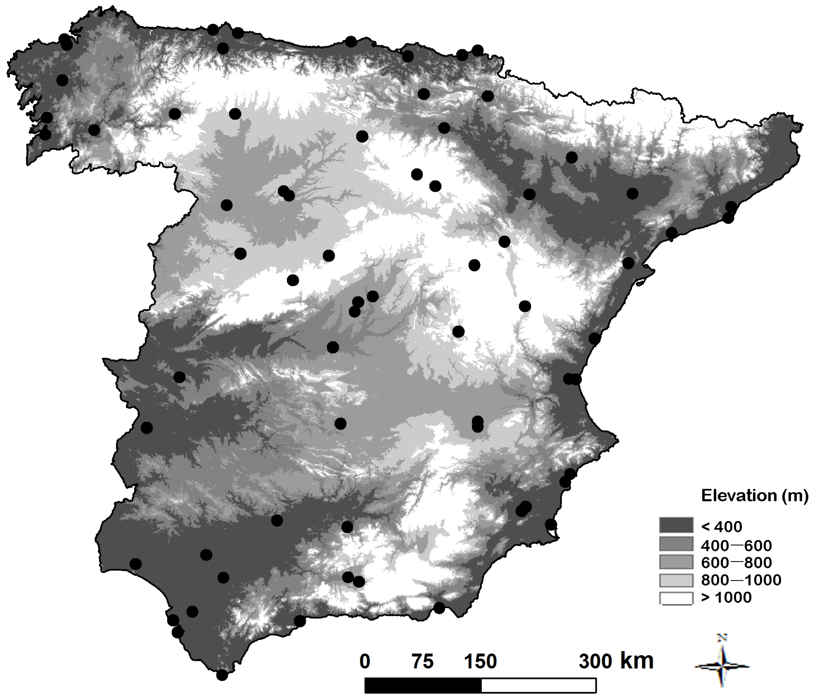
Daily meteorological observations at 72 georeferenced weather stations (
Figure 1), all of them belonging to the Meteorology Agency of the Spanish Government, were obtained. A period of 40 years, from 1975 to 2015, was used in this work, which is much more than the optimal length for a series (30 years) recommended by the World Meteorological Organization with the aim of obtaining reliable climate data to make predictions [
22]. The raw spatial database for all weather stations contained their geographic coordinates (referenced at UTM coordinates), elevation, and daily temperature (mean, maximum, and minimum) for the period 1975–2015.
Since chill models require hourly input data, such data were calculated from daily minimum and maximum temperatures using the methodology proposed by Baldocchi and Wong [
8]. Winter chill hours were summed between November 1 and February 28. On a daily basis, the number of chill hours was computed taking into account the aforementioned constraints of each model.
Consequently, winter chill was computed using the Chilling Hours Model, the Utah Model, and the Positive Utah Model. Their units are Chilling Hours (CH) for the Chilling Hours Model, Utah Chill Units (UCU) for the Utah Model, and Positive Chill Units (UCU+) for the Positive Utah Model. The values of these three chilling models (CH, UCU, UCU+) were incorporated in the final database together with the aforementioned initial data. Later, a geographic information system (GIS), specifically ArcGIS (version 10; ESRI, Redlands, CA, USA), was used to visualize and analyze the information.
With the aim of estimating at any location, geostatistical algorithms were used. In this section, regression-kriging (the estimator used in the case study) is briefly introduced. More information about it can be found in, for instance, Hengl et al. [
23].
In regression-kriging, instead of directly estimating the considered variable (CH, UCU, and UCU+ in this study), the interpolation is performed in two steps: estimation of the trend and then kriging of residuals. These two components are added back together to give the final prediction. A simple linear regression analysis is performed in the first step between the observed value of the variable and the auxiliary variable (elevation) at all sampling locations. Later, residuals are computed as the difference between the observed or measured value of the variable and the estimate by the trend. Residuals retain the spatial variability of the variable and they can be estimated by ordinary kriging at any location. In consequence, any variable at a new unsampled point,
x, is estimated,
, using regression-kriging as follows:
where
cj are the coefficients of the estimated trend model;
vj(
x) is the jth predictor at location
x (for
j = 0, the term represents the value where the linear regression intercepts the ordinate axis);
p is the number of predictors;
wi(
x), are the weights determined by solving the ordinary kriging system of the regression residuals,
r(
xi), for the n sample points.
More accurate estimates can be generated by a regression-kriging algorithm when the auxiliary data are available at all locations [
24], as occurs with some geographical properties such as elevation, which can be extracted from a digital elevation model (DEM), in raster format at 1000 × 1000 m
2 resolution, for mainland Spain. In consequence, from data at sampling locations, i.e., weather stations, estimates at any other unsampled location can be obtained. Thus, a continuous surface over all of mainland Spain can be produced and values for each chilling model for every one of the resolution unit can be determined. Three digital models, one for each chilling index, in raster format at 1000 × 1000 m
2 resolution, were initially generated. All operations were performed in ArcGIS v.10.3 and geostatistical analysis was conducted with its extension Geostatistical Analyst.
3. Results
Initially, data distribution was described using some descriptive statistics (
Table 1). The median and mean values were similar for the three chilling models in mainland Spain and the skewness values were low, which was indicative of data coming from a normal distribution. Moreover, the wide difference between minimum and maximum values and the high coefficients of variation for the three chilling models denote the existence of high climatic spatial variability as was expected because of the locations of the different meteorological stations (
Figure 1).
Table 2 shows that the values of the winter chill obtained with the three chilling models are highly correlated across Spain. A similar correlation between CH and UCU was obtained by Luedeling and Brown [
25] in a worldwide study. The level of linearity of the different relationships and, in consequence, the level of similarity between the different chilling models is apparent, denoting that the three chilling models are functionally very similar, i.e., each model depicts similar spatial climate characteristics. As Luedeling et al. [
20] indicated, deciding which model is most effective is difficult without extensive experimental model comparisons or analyses of phenological records, since the biological processes underlying the breaking of dormancy and the influence of temperature on these processes are poorly understood. Consequently, all of these chilling models are merely proxies of winter chill, relying entirely on empirical evidence. Moreover, although the mean values of the chilling models are highly correlated, with colder conditions expected in higher elevations, each model has a different theoretical interpretation, so they are not directly comparable.
It is also shown in
Table 2 that relationships between elevation, latitude, and each chilling model are apparent, as could be expected. Alburquerque et al. [
11] reported similar good correlation between UCU and elevation in Murcia, a region in southeastern Spain. In consequence, elevation and altitude seem to be the auxiliary variables used to estimate the chilling hours throughout mainland Spain using the regression-kriging algorithm. The results of the stepwise regression (ordinary least square estimation) analysis showed that the coefficient of determination was 0.41 when elevation was the unique auxiliary variable. When elevation and latitude were considered, the coefficient of multiple determination was 0.53 and the correlation was significant. The linear regression function was: CH = −2812.601 + 0.001 Y + 0.898 h, where h is the elevation (m) and Y is the latitude (UTM coordinate). Other auxiliary variables, such as longitude and distance to water bodies, did not significantly contribute to improve the multiple linear regression since the coefficient of multiple determination was, in any case, lower or close to 0.53.
A multivariate geostatistical work was performed to estimate CH at any location in Spain. The regression-kriging algorithm, in which the linear regression was the one previously indicated, used as initial data for the main variable, CH, all values measured at each meteorological station. CH showed a clear spatial dependence (
Figure 2); the experimental variogram was calculated and a theoretical spherical variogram was fitted to their points. Analysis of spatial correlation of residuals showed that the range of the variogram was smaller and the sill was bounded (
Figure 2). This indicated that the drift had been removed. The spatial correlation structure described with the spherical variogram of residuals was integrated in the ordinary kriging algorithm to estimate CH residuals throughout Spain.
The accuracy of the kriged CH map was determined with a cross-validation process. The mean error, which evaluated the true prediction accuracy and was computed as the difference between estimated values and actual observations at each meteorological station, was 7.62. Moreover, the root mean square error, which evaluated the accuracy of the prediction, was 79.6. As the mean CH value was 831.8 (
Table 1), the root mean square error was lower than 9.5% of the mean value. Furthermore, when the observed CH values versus the predicted values were plotted, the points fell close to the 45-degree line (
Figure 3). Consequently, the CH map represents very closely the real spatial distribution of the winter chilling hours. This is in accordance with Hengl et al. [
26] who found that the accuracy of a model is higher when kriging of the residuals is incorporated in the prediction algorithm.
As was shown, the RK algorithm was used to directly estimate CH throughout Spain. However, another alternative was checked; temperature values were also interpolated and then computed CH. However, the mean error and the root mean square error were higher with this second alternative (13.87 and 257.63, respectively). In consequence, it was less effective and this option was not considered.
Finally, the map of kriged estimates provided a visual representation of the distribution of the CH in Spain (
Figure 4). A digital CH map, in raster format at 1000 × 1000 m
2 resolution, was finally generated. As correlations between CH, UCU, and UCU+ are very high, digital maps for UCU and UCU+ throughout mainland Spain were also obtained in raster format at the same resolution (1000 × 1000 m
2) after applying map algebra techniques. The linear relationships considered to perform the mathematical operations are shown in
Table 3. Both final digital maps for UCU and UCU+ in Spain are shown in
Figure 4.
Comparison of data at each location versus predicted values was also performed with the aim of providing an idea about the reliability of the final digital maps. Thus, it was revealed that predictions were reasonably accurate, since the correlation coefficients with respect to the straight line, y = x, were 0.81 and 0.82, for UCU and UCU+, respectively.
If quantile statistics for the three chilling models are calculated, that is, winter chilling measurements are divided into intervals with equal probabilities, considering each meteorological station and the 40 annual values, and they are related to the mean values, linear regressions with high coefficients of determination are expected. In this case study, all coefficients of determination were around 0.99, when the 25% and 75% quantiles were correlated with mean values. From the digital maps of mean values (
Figure 4), new 75% and 25% quantile maps (
Figure 5 and
Figure 6) were computed by using map algebra procedures.
Table 4 shows the percentage of the territory of mainland Spain, excluding the zones with an elevation higher than 1000 m, within each interval defined in
Figure 4. Mean CH are mainly in the higher intervals, above 900 CH, with more than 75% of the territory. If the quantile maps are considered, this percentage varies until around 66% and 81% for the 25% and 75% quantiles, respectively. The same was apparent when the UCU was taken into account. Mean UCU values above 1600 comprise around 59% of the territory, and around 48% and 70% for the 25% and 75% quantile maps, respectively. For UCU+ values, the distributions were also similar, being around 60% of the territory for values above 1600, and around 48% and 72% for the 25% and 75% quantile maps.
4. Discussion
The geographic location of each area has a decisive influence on the temperature and the chill accumulation that can be recorded. Moreover, it is important to denote how the use of single climate stations to represent the climate within a region is not adequate because they cannot accurately characterize the level of spatial variability. Consequently, it is necessary to use adequate interpolation algorithms to properly perform the analysis about the spatial patterns of the studied climatic variables. Luedeling and Brown [
25] compared some winter chill models for fruit and nut trees throughout the world, with a poor coverage in many areas worldwide. However, the resolution of the maps they provided was not sufficient to accurately delineate chilling hours at national or regional levels. For instance, the distribution of chilling hours in Spain was too general, with only two or three classes throughout its territory.
Using the multivariate geostatistical algorithm, as regression-kriging, and considering elevation and latitude as the auxiliary variables because of their good correlation with the amounts of winter chilling, the spatial distributions of CH, UCU, and UCU+ have been accurately delimited in the mainland Spain.
Growers of fruit trees in temperate climates have to select tree cultivars with the correct chilling requirements for a particular zone. Thus, for an economically viable production, cultivars of the different fruit tree species, such as, for instance, cherry, peach, plum, apple, pear, almond, or walnut, have their specific chilling requirements and, consequently, winters in the production zone must be sufficiently long and cold to satisfy the required winter chill. In this sense, the quantile maps are particularly useful tools to estimate different areas with similar accumulation of winter chill with a confidence level. For example, if a 25% quantile map is considered, areas in which the estimates are performed will have that accumulation of winter chill with a high probability during at least the 75% of the years.
Alburquerque et al. [
11] analyzed the probability of satisfying the chilling requirements at different elevations for some cherry cultivars, but without showing the potential spatial distribution of them in the studied region. To illustrate the usefulness of the high-resolution digital maps to delineate and visualize the adequate areas in which different cultivars can satisfy their chilling requirements, the same particular case of some sweet cherry cultivars is utilized, since Spain is an important producing area, with around 33,000 ha [
5]. The sweet cherry cultivars used in the Spanish regions are very different because of new cultivars which have been introduced from other countries and their different chilling requirements.
Considering the values of the CH reported by Alburquerque et al. [
11] and Azizi Gannouni et al. [
27], the potential spatial distribution of three cherry cultivars (“Burlat”, “Marvin”, and “Sunburst”) growing in Spain is shown in
Figure 7. The earliest flowering cultivar is “Burlat”, which requires around 620 CH; the Californian cultivar “Marvin” requires around 790 CH and “Sunburst” is a cultivar with a higher chilling requirement at around 1040 CH.
Taking into account the CH kriged map shown in
Figure 7, obtained after considering mean CH values, “Burlat” could be potentially cultivated in almost every location of mainland Spain, except on the Mediterranean coast, close to the sea, and in the south, in the Guadalquivir valley and the area close to the Atlantic Ocean, where the chilling requirements would not be satisfied. Consequently, 71.2% of the total area of mainland Spain (zones higher than 1000 m are excluded) are potentially suitable for “Burlat”. The potential spatial distribution of “Marvin” would be smaller (
Figure 7); due to the high mean elevation of the Iberian Peninsula, it is around 63.4% of the Spanish territory under 1000 m. The higher chilling requirement of “Sunburst” determines that around 45.6% of the area of Spain under 1000 m is potentially suitable for this cultivar, which is an important percentage of the considered territory (
Figure 7). The three cultivars could be grown in this last percentage of the territory of mainland Spain, above an elevation around 460 m, where their chilling requirements would be guaranteed. Furthermore, the wide central plateau (Meseta Central) in Spain, with a mean elevation around 660 m, where winters are very cold, also guarantees a great number of chilling hours in a considerable area.
If a higher probability of satisfying the chilling requirements is desired, the 25% quantile map can be used to delineate the potential distribution of the sweet cherry cultivars (
Figure 8), as it is likely that during 75% of the years, the requirements of winter chilling is achieved, that is, this metric defines the minimum amount of winter chill that growers can expect in 75% of all years. Thus, 66.3%, 55.8%, and 35.5% of the total area of mainland Spain, excluding the zones higher than 1000 m, are potentially suitable for “Burlat”, “Marvin”, and “Sunburst”, respectively.
These maps are important tools to accurately delineate the areas in which different cultivars could be grown successfully. Particularly, those cultivars with low or medium chilling requirements are of great interest because they produce early harvests and fruit of higher quality without cracking problems, which are generated in areas with abundant rains [
28].
5. Conclusions
Climate information is usually related to individual stations, which is not representative of the true spatial climate patterns of a region. However, the accurate delineation of the spatial distribution of the main climate variables constitutes an important tool for decision making. In this work, the amount of winter chilling (based on three different models to measure its accumulation) throughout mainland Spain has been mapped using a GIS-based procedure.
Since accumulated chilling is mainly affected by the elevation at each location, this was utilized as an auxiliary variable to define different linear relationships between elevation and each chilling model. One of the novel aspects of this work is the use of a regression-kriging algorithm to estimate the chilling hours at any location, which could be performed by the significant linear relationships previously indicated.
Knowledge of the spatial distribution of the accumulated winter chilling is of great interest when deciding which different fruit tree species and cultivars are more suitable in a given area. Moreover, the probability of satisfying the chilling requirements can also be considered to delineate the appropriate zones.
One important characteristic of the present work is that it is based on data from the most recent time period—from 1975 to 2015. Furthermore, as far as we know, there is no similar work worldwide in which this broad and up-to-date temporal series has been used for zoning of a region or country considering the accumulation of winter chilling.
Further work could involve the application of these maps to analyze the potential spatial distribution of the most important fruit trees and cultivars across mainland Spain, completing our knowledge of the adaptability of different species where their culture has not been traditional.


 ,
, 


