A New Index Assessing the Viability of PAR Application Projects Used to Validate PAR Models

Abstract

Photosynthetically active radiation (PAR) is a useful variable to estimate the growth of biomass or microalgae. However, it is not always feasible to access PAR measurements; in this work, two sets of nine hourly PAR models were developed. These models were estimated for mainland Spain from satellite data, using multilinear regressions and artificial neural networks. The variables utilized were combinations of global horizontal irradiance, clearness index, solar zenith angle cosine, relative humidity, and air temperature. The study territory was divided into regions with similar features regarding PAR through clustering of the PAR clearness index (k_PAR). This methodology allowed PAR modeling for the two main climatic regions in mainland Spain (Oceanic and Mediterranean). MODIS 3 h data were employed to train the models, and PAR data registered in seven stations across Spain were used for validation. Usual validation indices assess the extent to which the models reproduce the observed data. However, none of those indices considers the exceedance probabilities, which allow the assessment of the viability of projects based on the data to be modeled. In this work, a new validation index based on these probabilities is presented. Hence, its use, along with the other indices, provides a double and thus more complete validation.

1. Introduction

In recent years, the growing global demand for food and biomass crops has pushed the research efforts to learn more about the factors that affect the growth and production of different crops in order to improve agricultural productivity. In this context, researchers seek not only to improve the efficiency of the processes involved in classical food crops, but they also aim to find new, clean and eco-friendly sources of power, such as obtaining biofuels and bioalcohols from biomass and the potential uses of microalgae in bioreactors. Microalgae are a promising field of study of the so-called third-generation biofuels that can contribute to reducing greenhouse gas emissions since they are non-polluting and sustainable. For instance, there is an ongoing project called the development of advanced technologies of microalgae for a circular economy (ALGATEC-CM S2018/BAA-4532) that addresses the coupling of biofuel production with the extraction of high-added value products to achieve the economic viability that microalgae technology needs. The effectiveness of the microalgae growth is mainly determined by the availability and concentration of nutrients as well as by the climatic variables, especially temperature and the ranges of photosynthetically active radiation (PAR) that are the best for biofuel or bioalcohol production. To this effect, modeling and simulating PAR and temperature conditions are key tools for the researchers involved in this project to discern which are the most suitable places to locate an outdoor pilot plant.

All types of crops need photosynthesis to grow and produce the leaves, fruits, or any type of bioproduct that interests us. Thus, controlling the ambient conditions to optimize photosynthesis is a key concern for researchers and technicians who seek to improve agricultural productivity. For instance, PAR is among the main variables to bear in mind when assessing the growth of biomass [1,2,3] or microalgae [4,5,6,7]. Many greenhouses use artificial lamps to replicate solar light, and there is an interesting field of research exploring the best lamp spectrum for different crops [8,9]. PAR is also of interest for gross primary production (GPP) [10], terrestrial net primary production (NPP) [11], and PAR use efficiency [12]. PAR optical properties are also a factor to bear in mind when choosing a cover for a greenhouse [13,14]. PAR is commonly defined as the band of solar spectrum located between 400 and 700 nm [15,16] because this portion of the solar spectrum is used by plants to convert light energy into biomass through photosynthesis.

However, acquiring PAR measurements is not always possible, since stations that provide PAR data are scarce or do not cover the desired extension of the field. Thus, an interesting option when PAR measurements are not available is to use PAR models. It is possible to sort these models of the bibliography depending on the nature of the data or the mathematical tool used to develop each model. Likewise, there are examples of satellite-derived models proposed in [17,18,19,20,21,22,23,24,25,26,27,28]. Another approach is using Kato’s bands [29] to obtain PAR estimates [30,31]. On the other hand, data collected on the Earth’s surface, such as global horizontal irradiance (GHI), air temperature (T), relative humidity (RH), sky clearness, skylight brightness parameter, and clearness index (k_t), can also develop PAR models [32,33,34,35,36,37,38]. It is also possible to train artificial neural networks (ANNs) to produce PAR estimates [39,40,41].

Different statistics are usually employed to validate the models’ performance, such as the mean bias error (MBE), the root mean square error (RMSE), the determination coefficient (R²), or the slope and the intercept of the linear regression between observed and modeled values. These statistics compare each observed value against the corresponding modeled value, so they assess the extent to which the models adequately reproduce the observed data. However, none of them takes into account the probabilities of exceedance that are usually employed to assess the viability of solar projects. These probabilities show the probability of exceeding a certain irradiance value [42]. For instance, P90 indicates an exceedance probability of 90%, which means that this irradiance value is exceeded 90% of the time. In other words, this value corresponds to percentile 10 of the variable. In this regard, three exceedance probability scenarios are recommended in [43] (P50, P90, or P99). In this work, we propose a validation index for models, based on these probabilities, so that those models that show a better value of this index will be more representative of the degree of viability that can be expected for a future project which uses PAR. As mentioned, the usual validation indices estimate the closeness of the model to the observed data point by point, so the model can be used to estimate the PAR-specific value, which can be used, to estimate outcomes based on this variable, such as the biomass productivity. Thus, a good model according to these indices must also be representative of the degree of viability of the project, but it is possible that a bad model according to these indices turns out to adequately represent that viability.

Thus, the objectives of this work are:

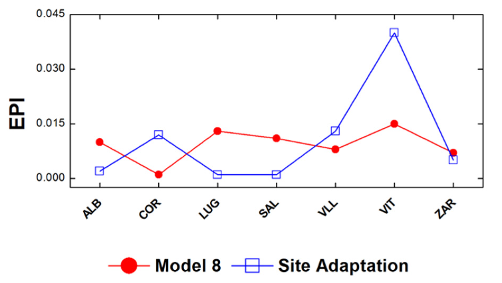
• To present a methodology to develop PAR models based on satellite data provided by a Moderate-Resolution Imaging Spectroradiometer (MODIS). The models’ development utilized data from each cluster to be specific for each region. Subsequently, a site adaptation technique was applied to the best models to test if there was an improvement in the results.
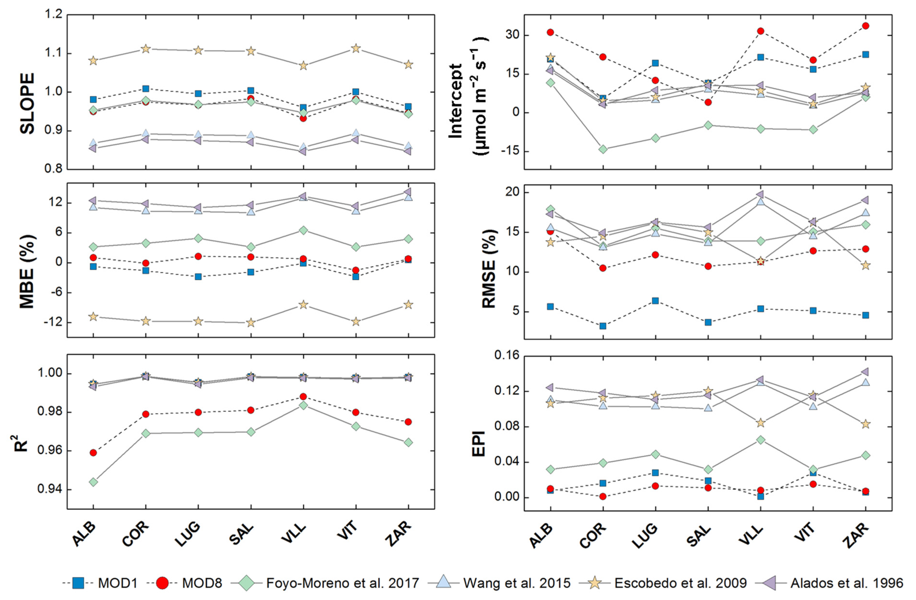
• To introduce a statistical index to assess the goodness of the developed models. This index is defined in Equation (12) (PAR could be replaced by any other modeled variable) and allows the estimation of the goodness of a model. Utilizing the defined Exceedance Probability Index (EPI), we can make a joint comparison of all those exceedance probabilities corresponding to modeled and measured values.

2. Materials and Methods

Two datasets were used; the first one was utilized for the development and the second one for the training of the models. GHI and PAR training data were downloaded from MODIS Land Products (MCD18) [44], particularly, the products handled were MCD18A1 [45] and MCD18A2 [46], respectively. This dataset covers a grid from 35.3° N to 44.0° N in latitude and from 9.5° W to 3.5° E in longitude. It has a resolution of 5 km (0.045 × 0.045°) and covers the period from 1 January 2018 to 31 December. Hourly T and dew point (T_d) data were provided by the European Centre for Medium-Range Weather Forecasts (ECMWF) [47]. These data cover a grid from 35.3° N to 44.0° N in latitude and from 9.5° W to 3.5° E in longitude. In this case, the resolution was 11 km (0.1 × 0.1°) from 1 January 2018 to 31 December 2018. These grids correspond to the location of the Iberian Peninsula where mainland Spain is located.

Data from seven PAR measurement stations belonging to the GEOPAR project (Project CGL2016-79284-P AEI/FEDER/UE) were used to validate the models. These stations provide PAR, GHI, RH, and T minute data. Each of these stations includes Apogee SP-110 and Apogee SQ-110 pyranometers for GHI and PAR measuring, respectively, and a HOBO S-THB Temperature/Humidity M002 psychrometer for RH and T measuring. Figure 1 illustrates the locations of these stations, and

Table 1. Localization of PAR stations.

Station	Abbreviation	Latitude (°, +N)	Longitude (°, +E)
Albacete—ITAP	ALB	39.04	−2.08
Córdoba—IFAPA	COR	37.86	−4.80
Lugo—USC	LUG	43.00	−7.54
Salamanca—CIALE	SAL	40.98	−5.72
Villaviciosa—SERIDA	VLL	43.48	−5.44
Vitoria—NEIKER	VIT	42.85	−2.62
Zaragoza—AULA DEI	ZAR	41.73	−0.81

summarizes these data.

For obtaining RH data to develop the models, T and T_d data provided by ECMWF were used according to Equation (1), derived from the Magnus formula and the Arden Buck Equation [48].

$$RH=100\cdot e^{\frac{b\cdot T_d}{c+T_d}-\left(b-\frac{T}{d}\right)\cdot \left(\frac{T}{c+T}\right)}$$

(1)

where RH is the relative humidity, T the air temperature, T_d is the dew point, b = 18.678, c = 257.14 °C, and d = 234.5 °C.

The clearness index (k_t) and solar zenith angle cosine (cos θ) were also employed for developing and validating the models. These variables were calculated following Equations (2) and (4).

$$k_t=\frac{GHI}{G_0}$$

(2)

where G₀ is the hourly global extraterrestrial irradiance, calculated as Equation (3) indicates:

$$G_0=I_{SC}\cdot \epsilon \cdot \frac{24}{2\pi }\left(\sin \varphi \cdot \sin \delta \cdot \left({\omega }_f-{\omega }_i\right)+\cos \varphi \cdot \cos \delta \cdot \left(\sin {\omega }_f-\sin {\omega }_i\right)\right)$$

(3)

where I_SC is the solar constant and equal to 1367 Wm⁻², ϕ the latitude, ω_i the hour angle at the beginning of the measurement period, ω_f the hour angle at the end of the measurement period, δ the declination angle, and ε the eccentricity of the terrestrial orbit [49,50].

$$\cos \theta =\sin \varphi \cdot \sin \delta +\cos \varphi \cdot \cos \delta \cdot \cos \omega$$

(4)

where ω refers to the hour angle.

To obtain the models, multilinear regressions and ANNs were used. ANNs are a machine learning technique proposed by [51], inspired by the connections of biological neurons. Briefly, this technique consists of an iterative process in which the network assigns different weights to the input signals until it reaches the nearest output to a target dataset [52,53,54]. This process is the so-called network training, once the ANN is trained can be fed with inputs to produce an estimated value.

The raw data from MCD18A1 [45] and MCD18A2 [46] provided by MODIS are 3 h averages covering mainland Spain with a resolution of 5 km. Modified Akima’s piecewise cubic Hermite interpolation [55,56] helped to produce hourly estimates based on MODIS data. Then, this estimated hourly dataset served to train different types of models. The proposed methodology is focused on developing regional models. With that purpose, the use of a clustering of the field of study contributed to constructing models for a whole region. This methodology employs a clustering of k_PAR, defined as the ratio between global extraterrestrial PAR (PAR₀) and PAR reaching the Earth’s surface, to separate the territory of study into two areas with similar characteristics.

A clustering served to establish the regions with similar behavior of PAR. The clustering was applied to k_PAR, defined in Equation (5).

$$k_{PAR}=\frac{PAR}{PA{R}_0}$$

(5)

where the PAR₀ value was estimated as 39.8% of G₀ according to [57,58].

The clustering technique employed was the k-means method, which consists of minimizing the sum of squared distances between the centroid of the group and each object of this group. There are many clustering methods, but k-means represents a widely used method, and its results over mainland Spain fitted well with the orographic and climatological characteristics of the territory. The clustering divided the field of study into two regions with similar behavior of k_PAR.

Once the regions with similar behavior were set, the development of both multilinear regression and ANN models for each region begun. The models were prepared using data provided by MODIS and ECMWF from all the points of the grid belonging to each region and subsequently validated with data provided by the stations located in the corresponding region.

The set of variables used in each model was the same for both multilinear regression and ANN models, as

Table 2. Set of variables used in each model.

	Multilinear Regression	ANN
Model 1	GHI	GHI
Model 2	GHI, kt	GHI, kt
Model 3	GHI, kt, cos θ	GHI, kt, cos θ
Model 4	GHI, RH, T	GHI, RH, T
Model 5	GHI, RH, T, kt, cos θ	GHI, RH, T, kt, cos θ
Model 6	kt·cos θ	kt·cos θ
Model 7	kt·cos θ, GHI	kt·cos θ, GHI
Model 8	kt·cos θ, RH, T	kt·cos θ, RH, T
Model 9	kt·cos θ, GHI, RH, T	kt·cos θ, GHI, RH, T

explains. Combinations of sets of variables that are commonly used in the bibliography were selected as GHI, RH, T, k_t, cos θ, and the product k_t·cos θ. Examples of models that utilize these variables can be found in [25,26,32,33,34,38,39,40,41,59,60,61,62,63]. The aim making different combinations of them is to produce different models so that we can compare them and choose which model is the best and which variables are more interesting for PAR modeling. In the first five models, combinations of these variables always including GHI were utilized, since the presence of this variable is the key to obtaining good results according to [25]. However, in the last four models, the combination of variables always included the product of k_t and cos θ, as this product obtained promising results in [41].

Afterward, a site-adaptation technique, used normally to correct models using local data, was utilized to improve the results [25,64,65,66]. To perform a site-adaptation correction, Equation (6) was applied.

$$y_{newmod}=y_{\mathrm{mod}}-\left[\left(a-1\right)x_{local}+b\right]$$

(6)

where y_{new mod} is the corrected model value, y_mod is the value of the original model, x_local is a local measured value, and the coefficients a and b are the coefficients obtained in a linear fitting between measured and modeled values.

The statistics used to estimate the goodness of the models developed were the slope and the intercept of the linear regression between measured and modeled PAR, the mean bias error (MBE), the root mean square error (RMSE), and the determination coefficient (R²), whose expressions are shown from Equation (7) to Equation (11).

$$Slope=\frac{{\displaystyle \sum _{i=1}^n\left(PA{R}_{Modeled}-{\overline{PAR}}_{Modeled}\right)}\left(PA{R}_{Measured}-{\overline{PAR}}_{Measured}\right)}{{\displaystyle \sum _{i=1}^n{\left(PA{R}_{Measured}-{\overline{PAR}}_{Measured}\right)}^2}}$$

(7)

$$Intercept={\overline{PAR}}_{Modeled}-Slope\cdot {\overline{PAR}}_{Measured}$$

(8)

$$MBE=\frac{1}{n}{\displaystyle \sum _{i=1}^n\left(PA{R}_{Modeled}-PA{R}_{Measured}\right)}$$

(9)

$$RMSE=\sqrt{\frac{1}{n}{\displaystyle \sum _{i=1}^n{\left(PA{R}_{Modeled}-PA{R}_{Measured}\right)}^2}}$$

(10)

$$R^2=\frac{{\sigma }_{PAR-ModPAR-Mea}^2}{{\sigma }_{PAR-Mod}^2{\sigma }_{PAR-Mea}^2}$$

(11)

where n is the number of recordings, ${\sigma }_{PAR-Mod}$ is the variance of the modeled PAR, ${\sigma }_{PAR-Mea}$ is the variance of the measured PAR, and ${\sigma }_{PAR-ModPAR-Mea}$ is the covariance of both modeled and measured PAR.

Additionally, to estimate the goodness of the models from the point of view of their representativeness when assessing the viability of PAR projects, a new index was defined. Indeed, the new index—called the Exceedance Probability Index (EPI)—is based on the exceedance probabilities, which are widely utilized to evaluate the viability of solar power plant projects. The proposed EPI estimates the difference between the exceedance probabilities for the modeled and measured variable (PAR could be replaced by any other modeled variable) as Equation (12) indicates. This difference is normalized dividing by the exceedance probability of the measured variable. According to this expression, when the exceedance probabilities of the measured and modeled values are close, EPI tends to zero.

$$EPI=\frac{{\displaystyle \underset{PA{R}_T=PA{R}_{\min }}{\overset{PA{R}_T=PA{R}_{\max }}{\int }}abs\left(P\left(PA{R}_M>PA{R}_T\right)-P\left(PA{R}_O>PA{R}_T\right)\right)}}{{\displaystyle \underset{PA{R}_T=PA{R}_{\min }}{\overset{PA{R}_T=PA{R}_{\max }}{\int }}abs\left(P\left(PA{R}_O>PA{R}_T\right)\right)}}$$

(12)

where PAR_T is a threshold PAR value, PAR_min is the lower PAR value, PAR_max is the higher PAR value, PAR_M is the modeled PAR, and PAR_O is the measured PAR.

3. Results

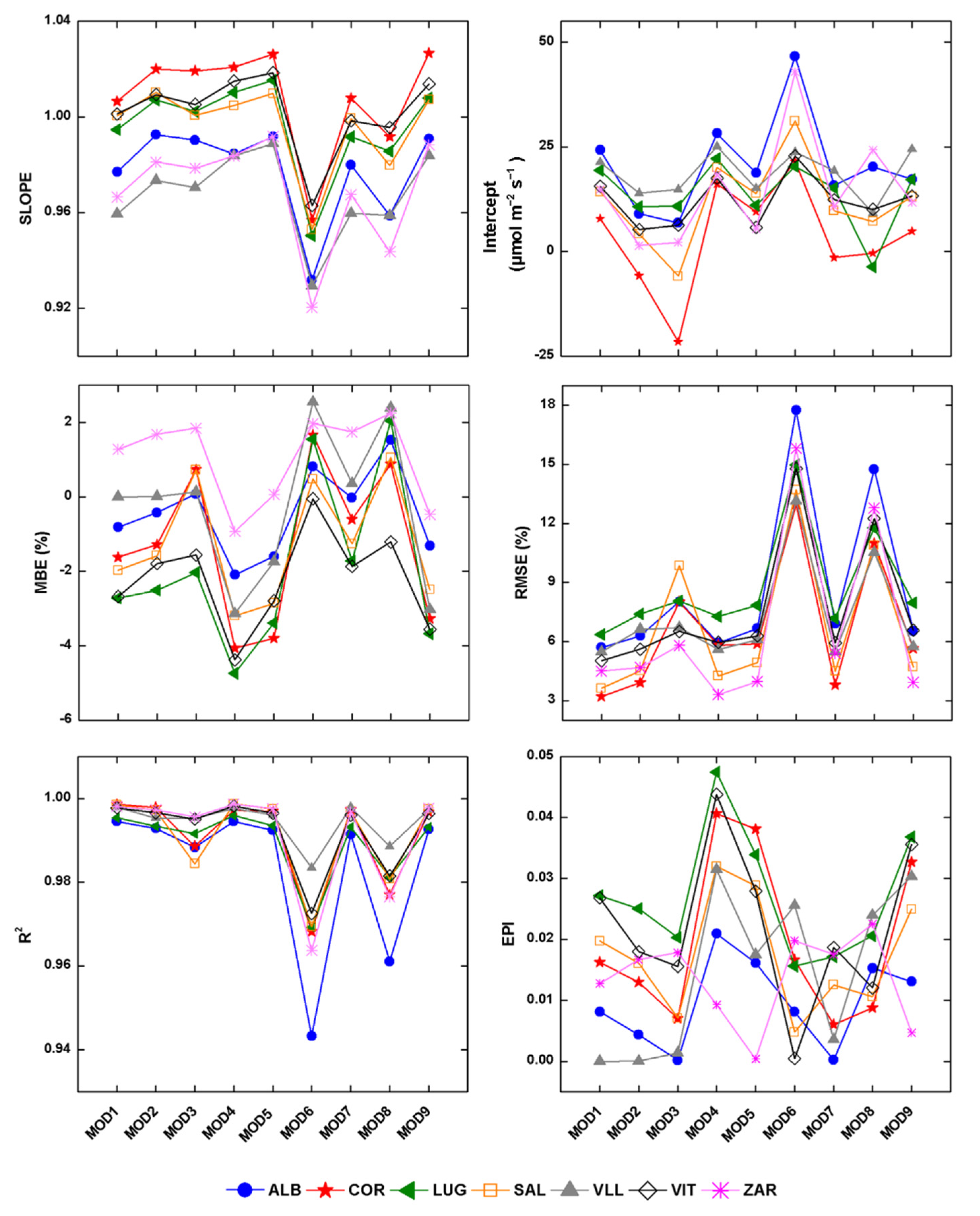
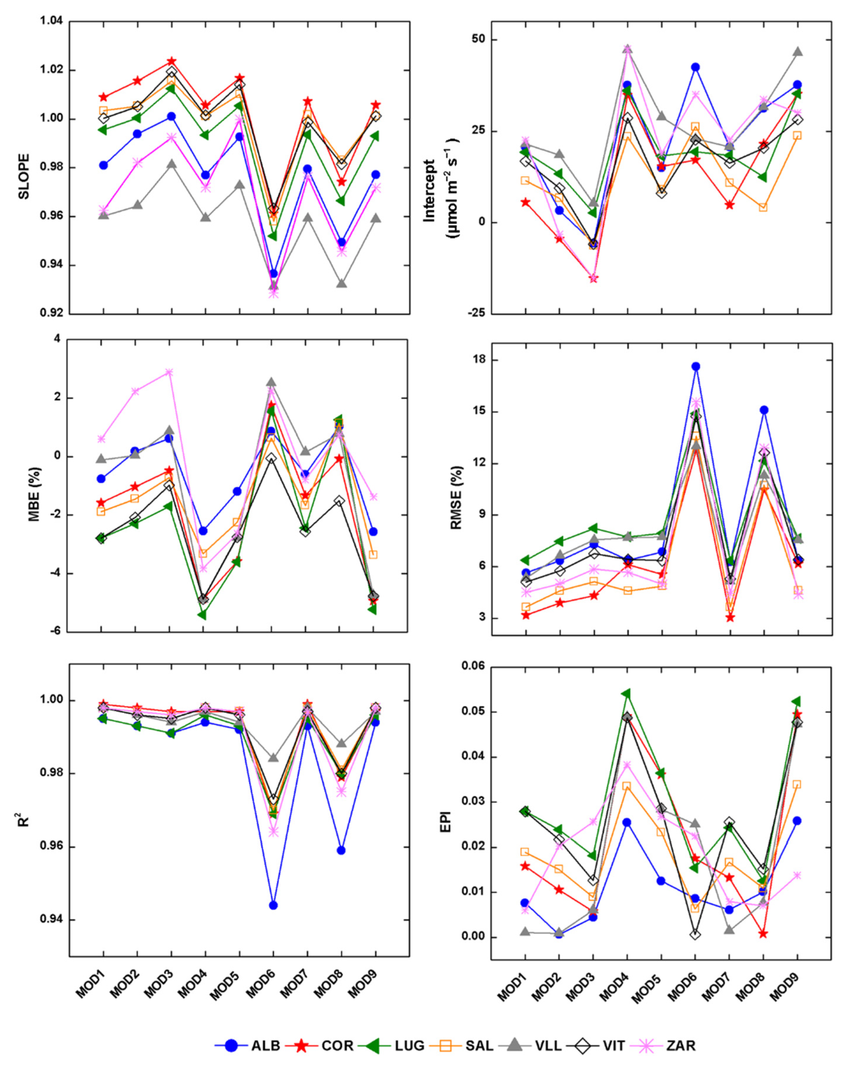
3.1. Regional PAR Models

The clustering of k_PAR conducted over the field of study permitted the development of regional PAR models. This procedure allows the separation of the field of study into regions that present similar behavior and characteristics concerning PAR. Hence, by using data from each cluster, it is possible to develop models for any place located in the area delimited by the cluster.

3.1.1. k_PAR Clustering

Figure 1 shows the division of the territory into two regions obtained after clustering k_PAR following the k-means method. The number of optimal clusters employed was two. Details of the method can be found in [58].

Compared to the climatological regions present in Spain [67,68], the two regions obtained throughout the clustering analysis fit with the Oceanic and the Mediterranean areas, respectively. Indeed, Oceanic climate is present in northern and northwest regions of Spain and fit reasonably with the green cluster, whereas eastern, southern, and central areas of Spain have a Mediterranean climate and fit well with the yellow cluster, though there are two different climatic varieties. In the eastern and coastal zones, the Mediterranean subtype is standard, and in the inner zones, the Mediterranean subtype is continental. In mainland Spain, there is another climate called the mountain climate. As its name indicates, this climate is typical of mountain ranges and high locations. This climate appears in mainland Spain in the main mountain ranges, such as the Pyrenees, Central Range, Iberian Range, and the Sierra Nevada. The cluster division did not account for this mountain climate, but the inclusions of the green cluster into the yellow cluster are located in the main mountain ranges in mainland Spain. This indicates that the mountain climate locations have been included in the green cluster [58,69].

According to this division, three stations are placed in the oceanic cluster: Lugo—USC; Villaviciosa—SERIDA; and Vitoria—NEIKER. However, the remaining four stations belong to the Mediterranean cluster (Albacete—ITAP; Córdoba—IFAPA; Salamanca—CIALE; and Zaragoza—AULA DEI). Therefore, the validation of the oceanic models employed only data from the three oceanic stations, and the validation of the Mediterranean models employed data from the other four stations.

Since the field of study was divided into two regions, there were only two sets of nine models generated, one set for the oceanic region and another set for the Mediterranean region. Thus, the same set of equations was used for validating the three oceanic stations, and another set of equations was utilized for validating the Mediterranean stations, as

Table 3. Equations of the nine models for each region.

	Oceanic Cluster	Mediterranean Cluster
Model 1	$PAR=13.81+2.02GHI$	$PAR=1.37+2.04GHI$
Model 2	$PAR=40.93+2.15GHI-170.78k_t$	$PAR=41.46+2.14GHI-158.21k_t$
Model 3	$\begin{array}{l}PAR=-15.37+2.01GHI-76.16k_t\\ +112.38\cos \theta \end{array}$	$\begin{array}{l}PAR=-22.74+2.00GHI-65.58k_t\\ +134.37\cos \theta \end{array}$
Model 4	$\begin{array}{l}PAR=-94.91+1.99GHI+0.91RH\\ +4.09T\end{array}$	$\begin{array}{l}PAR=-144.66+2.01GHI+1.32RH\\ +4.96T\end{array}$
Model 5	$\begin{array}{l}PAR=-83.20+2.01GHI+0.64RH\\ +3.31T-81.38k_t+82.15\cos \theta \end{array}$	$\begin{array}{l}PAR=-127.69+2.00GHI+1.07RH\\ +4.22T-68.19k_t+85.44\cos \theta \end{array}$
Model 6	$PAR=29.07+2637.98k_t\cdot \cos \theta$	$PAR=31.07+2634.29k_t\cdot \cos \theta$
Model 7	$\begin{array}{l}PAR=14.02+194.87k_t\cdot \cos \theta \\ +1.87GHI\end{array}$	$\begin{array}{l}PAR=1.86+178.16k_t\cdot \cos \theta \\ +1.90GHI\end{array}$
Model 8	$\begin{array}{l}PAR=115.40+2501.47k_t\cdot \cos \theta \\ -1.46RH+3.92T\end{array}$	$\begin{array}{l}PAR=115.09+2478.65k_t\cdot \cos \theta \\ -1.65RH+3.19T\end{array}$
Model 9	$\begin{array}{l}PAR=-90.38+63.03k_t\cdot \cos \theta \\ +1.94GHI+0.86RH+4.06T\end{array}$	$\begin{array}{l}PAR=-146.44-20.03k_t\cdot \cos \theta \\ +2.03GHI+1.34RH+4.98T\end{array}$

illustrates.

ANN setup had one input layer and one output layer, and the number of hidden layers was chosen according to the best performance reached. All ANNs were feedforward type and were fed with the set of inputs corresponding to each model. In total, 70 % of training data served to train the ANN, while the remaining 30 % of data validated the performance of the ANN to find the optimal number of hidden layers. In this case, the ANN training for each region utilized data from the corresponding region.

Validating with data from surface stations obtained the results illustrated in Figure 2 and Figure 3. The statistics utilized to evaluate the performance of the different models were the slope and intercept in a scatterplot, the mean bias error (MBE), the root mean square error (RMSE), and the EPI.

3.1.2. Site-Adaptation

To verify if the results obtained by Model 1 with MR—chosen as the best model for the first ranking—could be improved through a correction using local data, the site-adaptation technique for both the Mediterranean and Oceanic regions was applied. Likewise, this same technique was also applied to MR Model 8, as it was chosen as the best model for the second ranking, to check if an improvement could be achieved.

To obtain parameters a and b of Equation (6), half of the measured and modeled PAR data were fitted, and the other half of the data were used to validate the new model. Thus, half of the data randomly selected from Lugo—USC; Villaviciosa—SERIDA; and Vitoria—NEIKER were utilized to calculate a and b for the Oceanic region, and the same with data from Albacete—ITAP; Córdoba—IFAPA; Salamanca—CIALE; and Zaragoza—AULA DEI to calculate a and b for the Mediterranean region. The equation for the site-adaptation correction to the Oceanic region was (13), whereas for the Mediterranean region was Equation (14).

$$y_{newmod}=y_{\mathrm{mod}}-\left(0.01x_{local}-18.16\right)$$

(13)

$$y_{newmod}=y_{\mathrm{mod}}-\left(0.01x_{local}-14.85\right)$$

(14)

Figure 4 shows a comparison between the results of Model 1 (using MR) and site-adaptation correction, whereas Figure 5 shows a comparison between the results of Model 8 (using MR), which was chosen as the best one from the assessment carried out from the EPI, and site-adaptation correction.

4. Discussion

The clustering led to a division into two regions, one of them located in the north and northwest of mainland Spain and the other one located in the central, southern, and eastern areas of the territory. The division obtained in the clustering coincides with the two main climatological regions in mainland Spain [67,68]: Oceanic and Mediterranean. The northern cluster fits reasonably well with areas of Spain that have an oceanic climate, while the southern cluster coincides with the areas that have a Mediterranean climate. The presence of mountain ranges can explain the inclusions of the oceanic cluster in the Mediterranean one [58].

According to the results, it is not easy to infer what the best model is. It is necessary to assess all the statistics together to choose the best option. However, all the statistics used except the EPI are based on the comparison between the observed value and the corresponding modeled value. For its part, EPI is not based on a point-to-point comparison from which a compound index is obtained. Instead, the index is calculated comparing exceedance probabilities, which are the result of an entire set of points. Therefore, EPI is the best index to assess the goodness of a model that is going to be used to estimate the viability of a project. The rest of the statistics are used to assess the extent to which the model adequately reproduces the observed data. In that sense, for the evaluation of the models, we should use the EPI separately from the rest of the statistics, and propose two rankings of models: one focused on the degree of goodness when reproducing the observed data, and another focused on the goodness when assessing the viability of possible projects.

First, the models were ranked according to the first five statistics (the slope, the intercept, the R², the RMSE, and the MBE). Analyzing the performance of both MR and ANN models from the slope, R², and RMSE, the worst combination of variables is that of Models 6 and 8, that is, the models that did not include GHI as an input. As Figure 2 and Figure 3 illustrate, the slopes obtained with Models 6 and 8 either with MR or ANN for all the stations were the farthest from one. The same happened with the R²; the lower values were found in Models 6 and 8. Regarding RMSE, the highest values were obtained with Models 6 and 8. Indeed, the RMSEs of Models 6 and 8 were more than twice the RMSEs of the other models in the case of MR. The slope was close to one in the rest of the models. All the models obtained R² higher than 0.99, except Models 6 and 8. In the case of the RMSE, lower results were obtained with Models 1 and 7. According to the intercept, the worst models are 4 and 6 for both MR and ANN, and Model 9 in the case of MR whose intercepts were in all cases above 16 µmol m⁻² s⁻¹. On the other hand, the three best models are 1, 2, and 3, because their intercepts in all cases were below 25 µmol m⁻² s⁻¹. Regarding the MBE, the closest to zero per cent results were obtained with Model 8 when using MR, and Model 7 in the case of ANN; for these models, the MBE statistics were in all cases within the range (−2%–2%). However, the worst models according to their MBE are 4 and 9, since their numbers were the farthest to zero per cent in all cases. Thus, according to these five statistics (the slope, the R², the RMSE, the intercept, and the MBE), the best performance was obtained with Model 1, for both MR and ANN models.

Regarding the differences between ANN and MR models, in the case of the slope, they were not significant in Models 1, 2, 6, and 7. Model 3 was the only one in which the MR slopes were higher than ANN, and the difference between them was in the order of one hundredth in all stations. Inversely, the ANN slopes were higher than the MR slopes in Models 4, 5, 8, and 9; additionally, in these models, the largest differences reached three hundredths. Likewise, the differences between the intercepts of MR and ANN were not significant in Models 1, 2, 6, and 7. Only in Model 3 the ANN intercepts were above the MR intercepts (except in the case of Córdoba—IFAPA station); in the remaining models, MR intercepts were higher than ANN, and these differences reached the maximum in Model 9 where they were above 10 µmol m⁻² s⁻¹ for all stations and up to 30 µmol m⁻² s⁻¹ in Córdoba—IFAPA station. The differences between the R² obtained with MR and ANN were negligible, except in the case of Model 3 whose differences found on Córdoba—IFAPA and Salamanca—CIALE stations reached the order of one hundredth. Regarding the MBE, the differences were negligible in Models 1, 2, and 6. The largest differences in MBE were found in Model 9 (up to 1.71%), and the MBEs of ANN were closer to zero than the MBE of MR. In the case of RMSE, the differences were not significant in Models 1, 2, 6, and 8. In Models 4, 5, and 9, there were only significant differences in Villaviciosa—SERIDA and Zaragoza—AULA DEI stations. In Model 7, the RMSE of ANN was higher than the RMSE of MR. The largest differences (higher than 3.50%) were found in Model 3 in Córdoba—IFAPA and Salamanca—CIALE stations.

As the difference between Model 1 using ANN and MR was very small, Model 1 was chosen with MR as the best model because of its time of computation, which was more than two times lower compared to ANN.

The second ranking compared the EPI results. This index seemed to have similar behavior regarding the MBE and intercept, since EPI was determined from exceedance probabilities, that is, the complementary percentiles. If a model overestimates (or underestimates), its percentiles should be higher (or lower) than the observed data percentiles. Hence, EPI moved away from zero, the same as the MBE and intercept. Indeed, as happened with the intercept and MBE, in the case of EPI, the worst models were 4 and 9, whose average EPIs on all stations were, respectively, 0.043 and 0.039 for MR and 0.032 and 0.025 for ANN. The rest of the models were quite similar—except 5—obtaining EPI in the order of 0.01. However, Model 8 appeared as the best one of the MR models (its average EPI on all stations was 0.009), whereas for ANN models, Model 3 had the best EPI results by a narrow margin (its average EPI on all stations was 0.010). Thus, Model 8 with MR was chosen as the best model for the second ranking due again to its lower time of computation.

It is a remarkable fact that Model 8 is among the worst models according to the rest of the indices and that GHI is not an input variable for this model. As previously mentioned, the slope, the intercept, the R², the RMSE, and the MBE estimate the closeness of the model to the observed data point by point, so GHI is a necessary variable to adequately reproduce the PAR, as this variable is intrinsically associated with GHI (some PAR models are limited to expressing a ratio of GHI). In this work, the best combination of variables to achieve this purpose without GHI was the one proposed in Model 8 (k_t, cos θ, T, and RH). Nevertheless, though GHI is not used explicitly, in fact, it is utilized implicitly since k_t is defined as the ratio between the variables GHI and G₀. Thus, the information carried in GHI is one way or another needed to obtain good PAR estimates.

According to Figure 4, the results utilizing the site-adaptation technique improved slightly in Albacete—ITAP station. However, in the remaining stations, some statistics improved but others got worse. For instance, in Cordoba—IFAPA, the MBE improved, but the slope got worse, the same as in Vitoria—NEIKER, or in Villaviciosa—SERIDA and Zaragoza—AULA DEI where the slope improved but MBE worsened, whereas in Lugo—USC, the MBE improved, but the slope remained almost the same, and in Salamanca—CIALE, the MBE improved, but the slope got worse. In all cases, the intercept improved significantly using the site adaptation, whereas there were no significant differences in RMSE and R².

According to the EPI, the site adaptation improved the results in Albacete—ITAP, Lugo—USC, Salamanca—CIALE, and Zaragoza—AULA DEI, while in the remaining three stations, EPI got worse.

Bearing this in mind, it can be concluded that there was no clear improvement either by using the site-adaptation correction to Model 1—assessing the slope, the intercept, the R², the RMSE, and the MBE—or using the site-adaptation correction to Model 8—assessing the EPI.

Models 1 and 8 were compared to four hourly PAR models of the bibliography [32,34,41,59]. The following equations describe the models of the bibliography chosen for the comparison, where the coefficients were transformed to the units used in this work when needed:

In [41], the model in Equation (15) is proposed using the product of the clearness index (k_t) and the cosine of the solar zenith angle (cos θ).

$$PAR=2681.00\cdot k_t\cdot \cos \theta$$

(15)

The model described in Equation (16) was introduced in [59].

$$PAR=1.80\cdot GHI$$

(16)

Equation (17) shows the model suggested in [34].

$$PAR=2.24\cdot GHI$$

(17)

The last model was introduced in [32] and is expressed in Equation (18).

$$PAR=\left(1.83-0.19\cdot k_t+0.10\cdot \cos \theta \right)\cdot GHI$$

(18)

According to the results shown in Figure 6, the best performance of models found in the literature was reached with the model described in Equation (15). Comparing the slopes, in all the seven locations, the models closer to one were those obtained by the model proposed in [41]. No clear tendency on the intercepts was observed. Comparing the R², the models [32,34,59] were close to one in all the stations. However, the model proposed in [41] was further from one. Regarding the MBE statistics, the lowest values were also obtained using the model proposed in [41]. However, the lowest RMSE was obtained with the model proposed in [34] by a scarce difference. As far as EPI is concerned, the lowest results were those of the model proposed in [41]. The differences between the EPI of model [41] and the remaining models of the bibliography, which reached one magnitude order, are remarkable.

Comparing to the performance of Models 1 and 8, the slopes found with Model 1 were closer to one than those of the model proposed in [41], whereas the slopes obtained using Model 8 and the model proposed in [41] were quite similar. The intercepts of the model proposed in [41] were clearly closer to zero than those of Models 1 and 8, except in Córdoba—IFAPA and Salamanca—CIALE. Regarding R², the results of Model 1 were the closest to one, while those of Model 8 and the model proposed in [41] were similar. The MBE obtained with the model proposed in [41] was further from zero than in the case of Models 1 and 8. The same happened with RMSE, but in this case, the difference between the numbers of Model 1 and the model proposed in [41] was higher than the difference between Model 8 and the model proposed in [41]. Regarding EPI, the values of the model proposed in [41] were higher than those obtained in Models 1 and 8.

5. Conclusions

The new index allows the assessment of the viability of PAR projects, as it is based on exceedance probabilities, unlike the rest of the indices, which estimate the closeness of the model to the observed data point by point. Indeed, a good model according to these indices must also be representative of the degree of viability of the project, but it is possible that a bad model according to these indices turns out to adequately represent that viability. This is the case shown in the work, where Model 8 is the best model according to EPI, but it is one of the worst according to the rest of the indices. EPI adds information from a different point of view to the traditional statistics indices and could help in decision making to assess the suitability of PAR resources in an arbitrary location. EPI could be also useful for discerning which PAR model is more appropriate to estimate PAR in order to assess its potential regarding industrial exploitations such as agro-food cultivation, vegetables for biomass cultivation, or micro-algae cultivation to obtain biofuels.

A methodology for developing regional hourly models from 3 h satellite data was presented as well. The clustering utilizing k-means methods led to a division of the field of study into two regions with similar features regarding PAR. For each of these two regions, a set of nine multilinear regression and nine artificial neural network models was developed and validated.

As PAR is among the main variables to estimate the growth of biomass and microalgae, these models were validated bearing in mind that the viability of PAR projects can be applied to a priori estimate biomass production or the viability of a microalgae growth in different regions across mainland Spain, for instance. The clustering division of the territory fitted in with the two main climatic areas of Spain. This information will be useful in futures studies to assess the best species of microalgae cultivation according to the level of PAR irradiance received and the most suitable region to set it up.

The results showed small differences in the best models between multilinear regressions and artificial neural networks, but the higher time consumption of artificial neural networks made the multilinear regression models a better option. For the first ranking considered—indices which estimate the closeness of the model to the observed data point by point—all the models that did not include GHI as an input obtained the worst results, remarking the importance of GHI for PAR modeling in this case (the best performance was reached by Model 1, which only utilizes GHI as input). However, in the case of assessing the representativeness of a model when estimating the viability of a PAR project, GHI is not required explicitly for the model (Model 8), but indeed implicitly throughout k_t. This result illustrates that a model with traditional statistics, which can appear to be a bad model in the sense of replicating ground measurements, can be a good model from the point of view of the exceedance probabilities and may add valuable information for industrial exploitation.

A correction using a site-adaptation technique was introduced. The statistical results of the site adaptation to Model 1 and Model 8 improved some statistics but got worse in others. Thus, there was no clear improvement in the use of site adaptation in this case.

Finally, a comparison between Model 1 and 8 against four models of the bibliography was carried out. The results of the comparison showed that the performance of the models presented in this work was better than those of the bibliography, though the slopes and the R² of Model 8 and the model proposed in [41] were similar, and the intercepts of the model proposed in [41] were the lowest.

References

1. Hindersin, S.; Leupold, M.; Kerner, M.; Hanelt, D. Key parameters for outdoor biomass production of Scenedesmus obliquus in solar tracked photobioreactors. Environ. Boil. Fishes 2014, 26, 2315–2325. [Google Scholar] [CrossRef]
2. Hunt, E.R., Jr. Relationship between woody biomass and PAR conversion efficiency for estimating net primary production from NDVI. Int. J. Remote Sens. 1994, 15, 1725–1729. [Google Scholar]
3. Ramírez-Pérez, L.J.; Morales-Díaz, A.B.; de Alba-Romenus, K.; González-Morales, S.; Benavides-Mendoza, A.; Juárez-Maldonado, A. Determination of Micronutrient Accumulation in Greenhouse Cucumber Crop Using a Modeling Approach. Agronomy 2017, 7, 79. [Google Scholar] [CrossRef] [Green Version]
4. Kim, T.-H.; Lee, Y.; Han, S.-H.; Hwang, S.-J. The effects of wavelength and wavelength mixing ratios on microalgae growth and nitrogen, phosphorus removal using Scenedesmus sp. for wastewater treatment. Bioresour. Technol. 2013, 130, 75–80. [Google Scholar] [CrossRef]
5. Trofimchuk, O.A.; Petikar, P.V.; Turanov, S.B.; Romanenko, S.A. The influence of PAR irradiance on yield growth of Chlorella microalgae. IOP Conf. Ser. Mater. Sci. Eng. 2019, 510, 012017. [Google Scholar] [CrossRef]
6. Schmidt, J.J.; Gagnon, G.A.; Jamieson, R.C. Microalgae growth and phosphorus uptake in wastewater under simulated cold region conditions. Ecol. Eng. 2016, 95, 588–593. [Google Scholar] [CrossRef]
7. Vadiveloo, A.; Moheimani, N.R.; Cosgrove, J.J.; Bahri, P.A.; Parlevliet, D. Effect of different light spectra on the growth and productivity of acclimated Nannochloropsis sp. (Eustigmatophyceae). Algal Res. 2015, 8, 121–127. [Google Scholar] [CrossRef]
8. Rihan, H.Z.; Aldarkazali, M.; Mohamed, S.J.; McMulkin, N.B.; Jbara, M.H.; Fuller, M.P. A Novel New Light Recipe Significantly Increases the Growth and Yield of Sweet Basil (Ocimum basilicum) Grown in Plant Factory System. Agronomy 2020, 10, 934. [Google Scholar] [CrossRef]
9. Kowalczyk, K.; Olewnicki, D.; Mirgos, M.; Gajc-Wolska, J. Comparison of Selected Costs in Greenhouse Cucumber Production with LED and HPS Supplemental Assimilation Lighting. Agronomy 2020, 10, 1342. [Google Scholar] [CrossRef]
10. Wu, C.; Niu, Z.; Tang, Q.; Huang, W.; Rivard, B.; Feng, J. Remote estimation of gross primary production in wheat using chlorophyll-related vegetation indices. Agric. For. Meteorol. 2009, 149, 1015–1021. [Google Scholar] [CrossRef]
11. Pinker, R.T.; Zhao, M.; Wang, H.; Wood, E.F. Impact of satellite based PAR on estimates of terrestrial net primary productivity. Int. J. Remote Sens. 2010, 31, 5221–5237. [Google Scholar] [CrossRef]
12. Le Blon, B.; Guérif, M.; Baret, F. The use of remotely sensed data in estimation of PAR use efficiency and biomass production of flooded rice. Remote Sens. Environ. 1991, 38, 147–158. [Google Scholar] [CrossRef]
13. Cemek, B.; Demir, Y.; Uzun, S.; Ceyhan, V. The effects of different greenhouse covering materials on energy requirement, growth and yield of aubergine. Energy 2006, 31, 1780–1788. [Google Scholar] [CrossRef]
14. Lee, C.-S.; Hoes, P.; Cóstola, D.; Hensen, J. Assessing the performance potential of climate adaptive greenhouse shells. Energy 2019, 175, 534–545. [Google Scholar] [CrossRef] [Green Version]
15. McCree, K.J. Test of current definitions of photosynthetically active radiation against leaf photosynthesis data. Agric. Meteorol. 1972, 10, 443–453. [Google Scholar] [CrossRef]
16. Ross, J.; Sulev, M. Sources of errors in measurements of PAR. Agric. For. Meteorol. 2000, 100, 103–125. [Google Scholar] [CrossRef]
17. Chen, L.; Gao, Y.; Yang, L.; Liu, Q.; Gu, X.; Tian, G. MODIS-derived daily PAR simulation from cloud-free images and its validation. Sol. Energy 2008, 82, 528–534. [Google Scholar] [CrossRef]
18. Frouin, R.; Pinker, R.T. Estimating Photosynthetically Active Radiation (PAR) at the earth’s surface from satellite observations. Remote Sens. Environ. 1995, 51, 98–107. [Google Scholar] [CrossRef]
19. Zhang, Y.; He, T.; Liang, S.; Wang, D.; Yu, Y. Estimation of all-sky instantaneous surface incident shortwave radiation from Moderate Resolution Imaging Spectroradiometer data using optimization method. Remote Sens. Environ. 2018, 209, 468–479. [Google Scholar] [CrossRef]
20. Brown, M.G.L.; Skakun, S.; He, T.; Liang, S. Intercomparison of Machine-Learning Methods for Estimating Surface Shortwave and Photosynthetically Active Radiation. Remote Sens. 2020, 12, 372. [Google Scholar] [CrossRef] [Green Version]
21. Li, L.; Xin, X.; Zhang, H.; Yu, J.; Liu, Q.; Yu, S.; Wen, J. A method for estimating hourly photosynthetically active radiation (PAR) in China by combining geostationary and polar-orbiting satellite data. Remote Sens. Environ. 2015, 165, 14–26. [Google Scholar] [CrossRef]
22. Tripathy, M.; Raman, M.; Chauhan, P. Estimation of photosynthetically available radiation (PAR) from OCEANSAT-I OCM using a simple atmospheric radiative transfer model. Adv. Space Res. 2015, 56, 1441–1452. [Google Scholar] [CrossRef]
23. Janjai, S.; Wattan, R. Development of a model for the estimation of photosynthetically active radiation from geostationary satellite data in a tropical environment. Remote Sens. Environ. 2011, 115, 1680–1693. [Google Scholar] [CrossRef]
24. Van Laake, P.E.; Sanchez-Azofeifa, G. Simplified atmospheric radiative transfer modelling for estimating incident PAR using MODIS atmosphere products. Remote Sens. Environ. 2004, 91, 98–113. [Google Scholar] [CrossRef]
25. Ferrera-Cobos, F.; Vindel, J.; Valenzuela, R.; González, J. Models for estimating daily photosynthetically active radiation in oceanic and mediterranean climates and their improvement by site adaptation techniques. Adv. Space Res. 2020, 65, 1894–1909. [Google Scholar] [CrossRef]
26. Ferrera-Cobos, F.; Vindel, J.M.; Valenzuela, R.X.; González, J.A. Analysis of Spatial and Temporal Variability of the PAR/GHI Ratio and PAR Modeling Based on Two Satellite Estimates. Remote Sens. 2020, 12, 1262. [Google Scholar] [CrossRef] [Green Version]
27. Zhang, Y.; Liang, S.; He, T.; Wang, D.; Yu, Y.; Ma, H. Estimation of Land Surface Incident Shortwave Radiation From Geostationary Advanced Himawari Imager and Advanced Baseline Imager Observations Using an Optimization Method. IEEE Trans. Geosci. Remote Sens. 2020, 1–11. [Google Scholar] [CrossRef]
28. Huang, G.; Li, Z.; Li, X.; Liang, S.; Yang, K.; Wang, D.; Zhang, Y. Estimating surface solar irradiance from satellites: Past, present, and future perspectives. Remote Sens. Environ. 2019, 233, 111371. [Google Scholar] [CrossRef]
29. Kato, S.; Ackerman, T.P.; Mather, J.H.; Clothiaux, E.E. The k-distribution method and correlated-k approximation for a shortwave radiative transfer model. J. Quant. Spectrosc. Radiat. Transf. 1999, 62, 109–121. [Google Scholar] [CrossRef]
30. Nyamsi, W.W.; Espinar, B.; Blanc, P.; Wald, L. Estimating the photosynthetically active radiation under clear skies by means of a new approach. Adv. Sci. Res. 2015, 12, 5–10. [Google Scholar] [CrossRef] [Green Version]
31. Vindel, J.M.; Valenzuela, R.X.; Navarro, A.A.; Zarzalejo, L.F.; Paz-Gallardo, A.; Souto, J.A.; Méndez-Gómez, R.; Cartelle, D.; Casares, J.J. Modeling Photosynthetically Active Radiation from Satellite-Derived Estimations over Mainland Spain. Remote Sens. 2018, 10, 849. [Google Scholar] [CrossRef] [Green Version]
32. Alados, I.; Foyo-Moreno, I.; Alados-Arboledas, L. Photosynthetically active radiation: Measurements and modelling. Agric. For. Meteorol. 1996, 78, 121–131. [Google Scholar] [CrossRef]
33. Aguiar, L.J.G.; Fischer, G.R.; Ladle, R.J.; Malhado, A.C.M.; Justino, F.B.; Aguiar, R.G.; da Costa, J.M.N. Modeling the photosynthetically active radiation in South West Amazonia under all sky conditions. Theor. Appl. Clim. 2011, 108, 631–640. [Google Scholar] [CrossRef]
34. Escobedo, J.F.; Gomes, E.N.; Oliveira, A.P.; Soares, J. Modeling hourly and daily fractions of UV, PAR and NIR to global solar radiation under various sky conditions at Botucatu, Brazil. Appl. Energy 2009, 86, 299–309. [Google Scholar] [CrossRef]
35. Jacovides, C.; Boland, J.; Asimakopoulos, D.; Kaltsounides, N. Comparing diffuse radiation models with one predictor for partitioning incident PAR radiation into its diffuse component in the eastern Mediterranean basin. Renew. Energy 2010, 35, 1820–1827. [Google Scholar] [CrossRef]
36. Janjai, S.; Wattan, R.; Sripradit, A. Modeling the ratio of photosynthetically active radiation to broadband global solar radiation using ground and satellite-based data in the tropics. Adv. Space Res. 2015, 56, 2356–2364. [Google Scholar] [CrossRef]
37. Mizoguchi, Y.; Yasuda, Y.; Ohtani, Y.; Watanabe, T.; Kominami, Y.; Yamanoi, K. A practical model to estimate photosynthetically active radiation using general meteorological elements in a temperate humid area and comparison among models. Theor. Appl. Clim. 2013, 115, 583–589. [Google Scholar] [CrossRef]
38. Pashiardis, S.; Sa, K.; Pelengaris, A. Characteristics of Photosynthetic Active Radiation (PAR) Through Statistical Analysis at Larnaca, Cyprus. SM J. Biom. Biostat. 2017, 2, 1–16. [Google Scholar]
39. López, G.; Rubio, M.; Martínez, M.; Batlles, F. Estimation of hourly global photosynthetically active radiation using artificial neural network models. Agric. For. Meteorol. 2001, 107, 279–291. [Google Scholar] [CrossRef]
40. Jacovides, C.; Tymvios, F.; Boland, J.; Tsitouri, M. Artificial Neural Network models for estimating daily solar global UV, PAR and broadband radiant fluxes in an eastern Mediterranean site. Atmos. Res. 2015, 152, 138–145. [Google Scholar] [CrossRef]
41. Moreno, I.F.; Alados, I.; Alados-Arboledas, L. A new conventional regression model to estimate hourly photosynthetic photon flux density under all sky conditions. Int. J. Clim. 2017, 37, 1067–1075. [Google Scholar] [CrossRef] [Green Version]
42. Dobos, A.; Gilman, P.; Kasberg, M. P50/P90 Analysis for Solar Energy Systems Using the System Advisor Model. In Proceedings of the 2012 World Renew Energy Forum, Denver, CL, USA, 13–17 May 2012. [Google Scholar]
43. Fitch Rating. Rating Criteria for Solar Power Projects, Utility-Scale Photovoltaic and Concentrating Solar Power; Fitch Rating: New York, NY, USA, 2011. [Google Scholar]
44. Wang, D.; Liang, S.; Zhang, Y.; Gao, X.; Brown, M.G.L.; Jia, A. A New Set of MODIS Land Products (MCD18): Downward Shortwave Radiation and Photosynthetically Active Radiation. Remote Sens. 2020, 12, 168. [Google Scholar] [CrossRef] [Green Version]
45. Wang, D. MODIS/Terra+Aqua Surface Radiation Daily/3-Hour L3 Global 5km SIN Grid V006 [Data Set]. Available online: https://ladsweb.nascom.nasa.gov/ (accessed on 8 April 2020).
46. Wang, D. MODIS/Terra+Aqua Photosynthetically Active Radiation Daily/3-Hour L3 Global 5km SIN Grid V006 [Data Set]. Available online: https://ladsweb.nascom.nasa.gov/ (accessed on 8 April 2020).
47. Hersbach, H.; Bell, B.; Berrisford, P.; Biavati, G.; Horányi, A.; Sabater, J.M.; Nicolas, J.; Peubey, C.; Radu, R.; Rozum, I.; et al. ERA5 Hourly Data on Single Levels from 1979 to Present. Copernicus Climate Change Service (C3S) Climate Data Store (CDS). 2018. Available online: https://cds.climate.copernicus.eu/ (accessed on 17 April 2020).
48. Buck, A.L. New equations for computing vapour pressure and enhancement factor. J. Appl. Meteorol. 1981, 20, 1527–1532. [Google Scholar] [CrossRef] [Green Version]
49. Iqbal, M. An Introduction to Solar Radiation; Academic Press: Toronto, ON, Canada, 1983; ISBN 0123737508. [Google Scholar]
50. Sengupta, M.; Habte, A.; Kurtz, S.; Dobos, A.; Wilbert, S.; Lorenz, E.; Stoffel, T.; Renné, D.; Gueymard, C.A.; Myers, D.; et al. General Solar Position Calculations 2015. Sol. Energy 2020, 210, 20–37. [Google Scholar]
51. McCulloch, W.S.; Pitts, W. A logical calculus of the ideas immanent in nervous activity. Bull. Math. Biol. 1943, 5, 115–133. [Google Scholar] [CrossRef]
52. Gardner, M.W.; Dorling, S.R. Artificial neural networks (the multilayer perceptron)—A review of applications in the atmospheric sciences. Atmos. Environ. 1998, 32, 2627–2636. [Google Scholar] [CrossRef]
53. Priddy, K.L.; Keller, P.E. Artificial Neural Networks: An Introduction; SPIE: Bellingham, WA, USA, 2005. [Google Scholar]
54. Bengio, Y. Learning Deep Architectures for AI. Found. Trends Mach. Learn. 2009, 2, 1–127. [Google Scholar] [CrossRef]
55. Akima, H. A New Method of Interpolation and Smooth Curve Fitting Based on Local Procedures. J. ACM 1970, 17, 589–602. [Google Scholar] [CrossRef]
56. Akima, H. A method of bivariate interpolation and smooth surface fitting based on local procedures. Commun. ACM 1974, 17, 18–20. [Google Scholar] [CrossRef]
57. Magal, B.S. Solar Power Engineering; McGraw-Hill Education: New Delhi, India, 1999; ISBN 9780074518847. [Google Scholar]
58. Vindel, J.; Valenzuela, R.; Navarro, A.; Zarzalejo, L. Methodology for optimizing a photosynthetically active radiation monitoring network from satellite-derived estimations: A case study over mainland Spain. Atmos. Res. 2018, 212, 227–239. [Google Scholar] [CrossRef]
59. Wang, L.; Gong, W.; Feng, L.; Lin, A.; Hu, B.; Zhou, M. Estimation of hourly and daily photosynthetically active radiation in Inner Mongolia, China, from 1990 to 2012. Int. J. Clim. 2015, 35, 3120–3131. [Google Scholar] [CrossRef]
60. Yu, X.; Wu, Z.; Jiang, W.; Guo, X. Predicting daily photosynthetically active radiation from global solar radiation in the Contiguous United States. Energy Convers. Manag. 2015, 89, 71–82. [Google Scholar] [CrossRef]
61. Ren, X.; He, H.; Zhang, L.; Yu, G. Global radiation, photosynthetically active radiation, and the diffuse component dataset of China, 1981–2010. Earth Syst. Sci. Data 2018, 10, 1217–1226. [Google Scholar] [CrossRef] [Green Version]
62. Ren, X.; He, H.; Zhang, L.; Yu, G. Estimation of diffuse photosynthetically active radiation and the spatiotemporal variation analysis in China from 1981 to 2010. J. Geogr. Sci. 2014, 24, 579–592. [Google Scholar] [CrossRef] [Green Version]
63. Yu, X.; Guo, X. Hourly photosynthetically active radiation estimation in Midwestern United States from artificial neural networks and conventional regressions models. Int. J. Biometeorol. 2015, 60, 1247–1259. [Google Scholar] [CrossRef]
64. Aguiar, L.M.; Polo, J.; Vindel, J.; Oliver, A. Analysis of satellite derived solar irradiance in islands with site adaptation techniques for improving the uncertainty. Renew. Energy 2019, 135, 98–107. [Google Scholar] [CrossRef]
65. Polo, J.; Martin, L.; Vindel, J. Correcting satellite derived DNI with systematic and seasonal deviations: Application to India. Renew. Energy 2015, 80, 238–243. [Google Scholar] [CrossRef]
66. Vindel, J.M.; Polo, J.; Antonanzas-Torres, F. Improving daily output of global to direct solar irradiance models with ground measurements. J. Renew. Sustain. Energy 2013, 5, 063123. [Google Scholar] [CrossRef]
67. Bladé, I.; Cacho, I.; Castro-Díez, Y.; Gomis, D.; González-Sampériz, P.; Miguez-Macho, G.; Pérez, F.F.; Rodríguez-Fonseca, B.; Rodríguez-Puebla, C.; Sánchez, E.; et al. Climate in Spain: Past, Present and Future. Regional Climate Change Assessment Report of Clivar Spain; Pérez, F.F., Boscolo, R., Eds.; Ministerio de Medio Ambiente y Medio Rural y Marino; Ministerio de Ciencia e Innovación: Madrid, Spain, 2010; ISBN 978-84-614-8115-6. [Google Scholar]
68. Agencia Estatal de Meteorología (AEMET); Instituto de Meteorologia de Portugal (IM). Iberian Climate Atlas; AEMET-Ministerio de Medio Ambiente y Medio Rural y Marino & Instituto de Meteorologia de Portugal: Madrid, Spain, 2011; ISBN 978-84-7837-079-5. [Google Scholar]
69. Vindel, J.M.; Navarro, A.A.; Valenzuela, R.X.; Zarzalejo, L.F. Temporal variability patterns in solar radiation estimations. J. Atmos. Solar Terr. Phys. 2016, 143, 1–7. [Google Scholar] [CrossRef]
Figure 1. Result of kPAR clustering over the territory of study. The oceanic cluster is represented in green, while the Mediterranean one is in yellow. The locations of the seven stations used for validating the models are also represented.
Agronomy 11 00470 g001
Figure 2. Statistical results of the nine ANN models for each station.
Agronomy 11 00470 g002
Figure 3. Statistical results of the nine MR models for each station.
Agronomy 11 00470 g003
Figure 4. Comparison between the statistical results obtained by MR Model 1 and its site-adaptation correction.
Agronomy 11 00470 g004
Figure 5. Comparison between the statistical results obtained by MR Model 8 and its site-adaptation correction.
Agronomy 11 00470 g005
Figure 6. Comparison between Models 1 and 8 against bibliography models.
Agronomy 11 00470 g006