Abstract
Plot size has an important impact on variation among plots in agronomic field trials, but is rarely considered during the design process. Uniformity trials can inform a researcher about underlying variance, but are seldom used due to their laborious nature. The objective of this research was to describe variation in maize field trials among field plots of varying size and develop a tool to optimize field-trial design using uniformity-trial statistics. Six uniformity trials were conducted in 2015–2016 in conjunction with Iowa State University and WinField United. All six uniformity trials exhibited a negative asymptotic relationship between variance and plot size. Variance per unit area was reduced over 50% with plots 41.8 m2 in size and over 75% when using a plot size >111.5 m2 compared to a 13.9 m2 plot. Plot shape within a fixed plot size did not influence variance. The data illustrated fewer replicates were needed as plot size increased, since larger plots reduced variability. Use of a Shiny web application is demonstrated that allows a researcher to upload a yield map and consider uniformity-trial statistics to inform plot size and replicate decisions.
1. Introduction
Designing field experiments with adequate precision for detecting meaningful differences among treatments is challenging when the magnitudes of economic or biologically significant differences are small [1]. The power to test such differences depends not only on the magnitude of mean differences, but also on the chosen alpha level, the number of samples represented in each treatment mean, and the underlying variance among field plots for whatever measurement is being made [2].
The reciprocal relationship between experimental variance and field-plot size has been noted and studied by several researchers [3,4,5]. Smith [6] developed an empirical law for describing heterogeneity among field plots based on this nonlinear relationship:
where VS = variance of a plot of size s (area), V0 represents the theoretical maximum variance, and b is a soil heterogeneity index. The value of b ranges from zero to one. with the latter representing higher heterogeneity. A b value of one indicates the plots are spatially uncorrelated and homogeneous. A b value of zero means that plots are perfectly correlated, in which case the variance between plots is constant and does not depend on plot size [7].
While the shape of the relationship has been shown to be similar across many sites, the values of V0 and b vary considerably with the field being sampled, and are influenced by the crop species and the variable measured. Experimental variation in maize grain yield is particularly influenced by plot size for a number of reasons with a higher variance observed among smaller plots. When plots are too small, they fail to encompass the natural variation occurring within a site. The greater the soil heterogeneity, the greater the variability will be among smaller plots. Smaller plots are also affected to a greater extent by harvest losses and measurement errors [7]. For example, when maize is planted at a population of nine plants m−2, the loss of a single ear from a 1 m2 plot can result in a yield loss of 11%. The loss of a single ear has much less impact as the plot size increases. Errors in measuring plot length have a similar impact. A 10 cm error in measurement can result in either including or excluding an ear from the calculation of grain yield. Such an error would be trivial in a large plot, but could have a large effect on grain yield estimated from small plots. Experiments with seed limitations may use smaller plots due to necessity, but experimental design often use small plots out of convenience and habit [7].
Border effects from neighboring plots are also greater in small plots, and plants adjacent to open alleys experience reduced interplot competition in acquiring sunlight, air movement, soil moisture, and nutrients [8]. Alley effects not uniformly distributed across treatments have been shown to influence treatment effects [9,10,11].
Parameters for Smith’s model were originally and traditionally have been estimated using uniformity trial data [12]. The general approach is to subdivide a field into relatively small units from which measurements are taken and then aggregated into plots of various sizes and shapes. The field is managed uniformly so differences among plots can be ascribed to spatial variation in soil [12]. The variance among plots of each size is determined and regressed against plot area using log–log linear regression:
Despite its usefulness, conducting a uniformity trial to obtain estimates of soil heterogeneity is time- and labor-consuming, and is a seldom-used practice. Available literature demonstrates the effect of plot size on data variance of maize from past decades [13,14,15,16], on inbreds [17], and from regions outside of the United States [18]. Continued advances in plant breeding and agronomic practices have resulted in increased average maize grain yield in the United States. Data is needed on current maize hybrids from key maize growing regions within the United States to inform researchers on best practices regarding experimental design decisions.
Further, developing a more robust and relatively simple method for acquiring the soil heterogeneity index for a given plot area would enable researchers to optimize plot size based on the competing constraints of cost and experimental precision. Georeferenced data could be used to estimate the parameters of Smith’s model more easily compared to conducting a formal uniformity trial, and perhaps with greater precision. The objectives of this research were to describe variation in maize yield among field plots of varying size using elite commercial germplasm grown under modern management practices from the Upper Midwest region of the United States to provide guidance for optimizing plot size for measuring yield, and to provide researchers with a web tool to automate data compilation for interpretation of uniformity trials conducted on their own research sites.
2. Materials and Methods
2.1. Site Characteristics and Trial Execution
Uniformity trials were conducted in 2015 and 2016 at the Iowa State University Agronomy Research Farm near Boone, IA, and near River Falls, WI, on a research site operated by WinField United (Land O’Lakes, Arden Hills, MN, USA). A description of the site characteristics and agronomic management practices for each site are included in Table 1. In all trials, an area roughly 0.3 ha−1 was bulk-planted with a single maize (Zea mays L.) hybrid in 76 cm rows. Herbicide and insecticide crop protection inputs were used at each site as needed to control weeds and pests, and were uniformly applied across the trial site. Seed was planted to a depth of 4 to 5 cm directly between the rows from the previous year using a planter equipped with row cleaners and 13-wave coulters positioned directly in front of the seed disk openers.

Table 1.
Agronomic management practices of six uniformity trials conducted to investigate the effect of plot shape and size on the variance of maize yield.
Alleys were cut following tassel emergence and pollination using a tractor guided by a global positioning system to divide the trial area into 12 ranges 4.6 m in length with a border on all sides. Plot size of 144 individual plots in a 12 × 12 grid measuring 3.0 m wide × 4.6 m long was measured to the nearest 12.7 mm. Harvest was performed using a Winterstieger combine (Winterstieger, Salt Lake City, UT, USA) equipped with a HarvestMaster GrainGage (Juniper Systems, Logan, UT, USA) providing yield and seed moisture measurements for the middle two rows. Plot yields were recalculated based on the actual plot size recorded prior to harvest.
Data were analyzed using the index.smith function from the agricolae [19] package within R software [20] to calculate Smith’s index of soil heterogeneity. Yield maps were interpolated from data collected by grid sampling as described above. Maps were created using the kriging interpolation Spatial Analyst tool of ArcMap 10.8 (ESRI, Redlands, CA, USA). A spherical semivariogram model was used with the ordinary kriging method to do the interpolation.
2.2. Uniformity-Trial Web Application
A web application was built using the shiny [21] package of R [20]. The user must upload a csv file with specific column headings: row, col, plot_width, plot_length, and yield. The plot_width, plot_length, and yield data may be in Imperial or SI units; the output will be returned in the same units.
The application returns three tab panels of information. The first tab panel, “Yield Map”, produces a basic plot map, which is simply a scatter plot created with the ggplot2 [22] package, using the col and row data as horizontal and vertical coordinates, and with points colored according to relative yield.
The second tab panel, “Smith’s Index”, uses the index.smith function of the agricolae [19] package to generate a uniformity table. The uniformity table contains every plot configuration possible, using multiples of the original plot lengths and widths. For each plot configuration, the variance among plots is calculated.
The regression of plot variance on plot area is then plotted using the ggplot2 [22] and plotly [23] packages, in which blue points represent actual plot variances, and a red line represents the variance predicted by Smith’s index. In addition, the natural logarithms of variance and plot size are fit with a linear regression model, and the slope is reported as Smith’s index below the plot.
The third tab panel, “LSD vs. Plot Size”, uses ggplot2 [22] to display the regression of least significant difference (LSD) at the α = 0.05 level of significance. LSDs are displayed assuming two, three, four, five, or six replications, and are calculated from the variance predicted by Smith’s index.
3. Results
3.1. Uniformity Trials
Maize yields from the six uniformity trials ranged from 7636 to 19,139 kg ha−1 (Figure 1), and the average difference between the minimum and maximum values within the trials was 6114 kg ha−1.
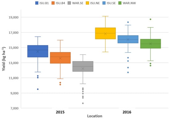
Figure 1.
Summary statistics for six maize uniformity trials conducted to investigate the influence of plot size and shape on soil heterogeneity. X denotes the mean, horizontal line denotes the median, the box (rectangle) represents the interquartile region (IQR), and the whiskers (vertical lines) represent the upper and lower quartiles, respectively. Dots are outliers defined as being outside 1.5 × IQR.
Variance per unit area decreased as plot size increased, and all six uniformity trials exhibited a negative asymptotic relationship between variance and plot size. Variance per unit area was reduced over 50% with plots 41.8 m2 in size, and over 75% when using a plot size >111.5 m2 compared to a 13.9 m2 plot (Figure 2).

Figure 2.
Estimated variance per unit area among plots of various sizes and shapes from six maize uniformity trials based on predicted values calculated from regression of log (variance) on log (length).
While the general shape of the curves was similar among all six sites, the degree of soil heterogeneity differed. The interpolated yield maps in Figure 3 illustrate the presence and degree of soil heterogeneity within each site.
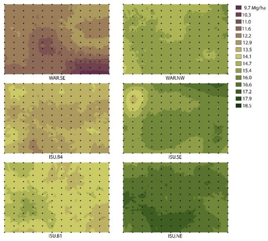
Figure 3.
Interpolated yield maps for six maize uniformity trials conducted from 2015–2016 to evaluate the natural variability among field plots of varying size. A total of 144 experimental units were arranged in a 12 × 12 grid with individual plots measuring 3.0 m wide × 4.6 m long. Maps were created using the kriging interpolation Spatial Analyst tool of ArcMap 10.8 (ESRI, Redlands, CA, USA). A spherical semivariogram model was used with the ordinary kriging method for the interpolation.
Smith’s index of soil heterogeneity ranged from 0.532 to 1.026 among the six trials (Table 2).

Table 2.
Estimates of Smith’s soil heterogeneity index (b), the natural logarithm of the base variance (V) estimated using ln–ln linear regression of variance on plot area. Means within columns followed by the same letter were not significantly different at p = 0.05.
The soil heterogeneity index combining data across the six trials was 0.75, indicating that these sites had a high degree of soil heterogeneity or low correlation between adjacent plots.
Plots of varying shapes were included in these uniformity trials for plot sizes of 27.9, 41.8, 55.7, 83.6, 111.5, 167.2, 250.8, and 334.4 m2. A Chi-squared test revealed the shape of the plot did not result in a statistically lower variance within a fixed plot size (data not shown). The data also illustrated the relationship between plot size and replicate number in influencing the ability to detect treatment differences (Figure 4).

Figure 4.
Relationship between plot size and least significant difference for trials with varying replicates using data from six uniformity trials conducted in the Upper Midwest region of the United States.
There was a tradeoff between these two design factors, and fewer replicates were needed as plot size increased, since larger plots had a lower variance. Based on the degree of soil heterogeneity present in these uniformity trials, a 111.5 m2 plot with two replicates will produce an equivalent least significant difference (LSD) compared to a 27.9 m2 plot with six replicates.
3.2. Uniformity-Trial Data Automation
Here, the data output of the Shiny application will be demonstrated for automation of uniformity-trial data compilation. Grain yields for fields ISU.B4 and ISU.SE are displayed, with data presented per experimental unit and points colored based on relative yield (Figure 5). The overall productivity of field ISU.B4 was lower, and the yield of individual plots more randomly distributed compared to ISU.SE.
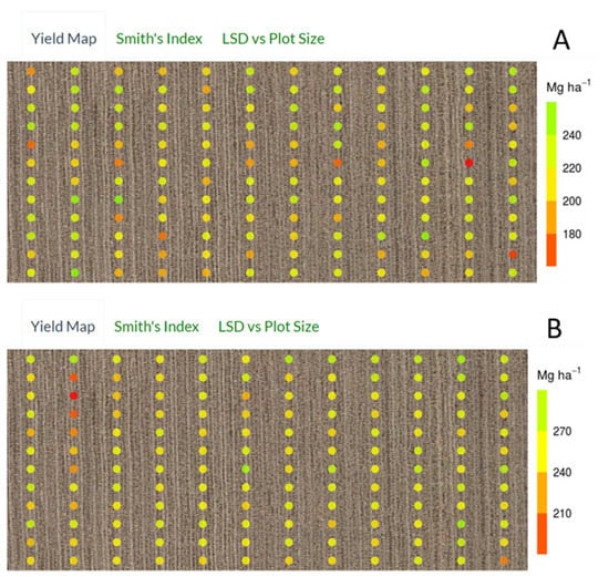
Figure 5.
Output from a Shiny application to automate data compilation for uniformity trials. The output data include a plot map with horizontal and vertical coordinates and points colored according to relative yield. Fields ISU.B4 (A) and ISU.SE (B) are used in this example. Relationship of Variance and Plot Size. Available online: https://marin-harbur.shinyapps.io/plot_size_app_for_uploaded_data/ (accessed on 18 June 2021).
Smith’s index of soil heterogeneity for field ISU.B4 was almost twice that of field ISU.SE (Table 2). Variances for all possible plot sizes and shapes were plotted, and a regression line fit based on Smith’s index. While both fields exhibited a negative asymptotic relationship between variance and plot size, the slope of the curve was much steeper for field ISU.B4, indicating that for initial small plot sizes, a change in plot size would be expected to have a large effect on variance (Figure 6). In contrast, changes in plot size for field ISU.SE would result in a less-dramatic change to plot variance, since the field had a lower value for Smith’s index.
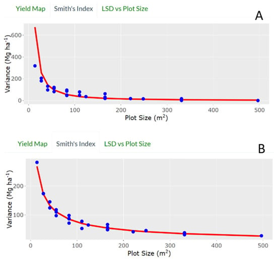
Figure 6.
Output from a Shiny application to automate data compilation for uniformity trials. The output data include Smith’s index along with a plot regressing plot variance on plot area. Fields ISU.B4 (A) and ISU.SE (B) are used in this example. Relationship of Variance and Plot Size. Available online: https://marin-harbur.shinyapps.io/plot_size_app_for_uploaded_data/ (accessed on 18 June 2021).
The third panel displays the regression of LSD based on plot size for trials with varying replicate scenarios (Figure 7). The data can aid a research practitioner planning out the design factors for an experiment, given the variation present in the field and available land. Using field ISU.B4 as an example, a trial with four replicates and plot size of 165.6 m2 will produce a similar LSD as a trial with 6 replicates and plot size of 91.6 m2.
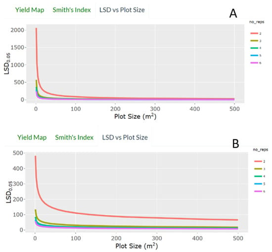
Figure 7.
Output from a Shiny application to automate data compilation for uniformity trials. The output data include the regression of least significant difference on plot size for trials with two, four, or six replicates. Fields ISU.B4 (A) and ISU.SE (B) are used in this example. Relationship of Variance and Plot Size. Available online: https://marin-harbur.shinyapps.io/plot_size_app_for_uploaded_data/ (accessed 18 June 2021).
4. Discussion
These data indicated that field characteristics at the same location but within different parts of the field exhibited unique characteristics. For example, field ISU.B4 exhibited the greatest index of soil heterogeneity (b), and the variation was oriented in a gradient going from the front of the trial to the back. Without adjustments to alpha levels, replicate number, or plot size, this site would be best suited for field trials with treatments with large, expected magnitudes of response. Prior knowledge of these gradients could allow for appropriate orientation of blocks to successfully partition variation from the residual variance. In contrast, field ISU.SE had one of the lowest soil heterogeneity values and a more neutral gradient. This field could accommodate a variety of trials, and would be a good choice to evaluate agronomic practices in which treatment differences are expected to be small. However, there was a problematic area within the field that should be omitted from trials.
The negative asymptotic relationship between variance and plot size agreed with findings from Smith [6] and others [16]. Some uniformity trials have shown plot-size trends that were contradictory to Smith’s Law of Heterogeneity [3,4]. However, the crops in those trials were perennial forage grasses, which present a very different cropping system compared to an annual maize system. Annual systems are subject to more-frequent disturbance from agronomic practices resulting from planting, maintenance, and harvest, in addition to new trials being placed over the top of past trials in successive years. In addition, maize can be particularly troublesome because the number of plants per plot is small, resulting in a large individual contribution to the overall plot yield [7].
Past trials investigating the effect of plot shape demonstrated inconsistencies in the ability for plot shape to lower experimental error [6,14,24]. These trials showed that plot size had no effect when the magnitude of soil variation was equal in both plot dimensions. The optimum plot shape should reduce differences in soil productivity from plot to plot within a block, and therefore requires knowledge of gradients within the trial site. Multistate field trials on corn (Zea mays L.), soybean (Glycine max (L.) Merr.), and sorghum [Sorghum bicolor (L.) Moench] showed that multiple gradients were prevalent in field trials [25]. Plots squarer in shape provided a safeguard to the experimenter if the presence and direction of gradients was not known.
The choice between adding more replicates versus increasing plot size is especially critical if there are land constraints for the trial area. Small plots increase experimental error and require a larger number of replicates, whereas larger plots reduce residual variance, requiring fewer replicate plots. While both design control factors influence experimental error, increasing replicates is considered most effective when soil heterogeneity coefficients are moderate (0.2 < b < 0.7), and increasing plot size is most effective in highly heterogenous settings (b > 0.7) [6].
While increasing replicates of small plots (≤27.9 m2) is an effective strategy to reduce variance, the benefit decreases with each additional replicate (Figure 4). Adding replicates to small plots also fails to address edge and alley effects, which can interact with treatment effects and confound results [10,11,12]. More plants in small plots (≤27.9 m2) are closer to plot alleys, which provides greater access to additional resources such as sunlight, soil moisture, and nutrients compared to larger plots, which can elevate the yield of plants toward plot ends [26]. Because larger plots reduce the perimeter-to-area ratio and a greater percentage of plants are away from alleys, per-plant yields could be lower, allowing more room for yield enhancement from agronomic inputs.
Tedford et al. [27] found the consistency and magnitude of response from foliar fungicide applications increased as plot size became larger. Kandel et al. [28] demonstrated that small plots and large plots could produce similar yield responses, but over twice as many replicates were needed when using small plots to detect the same treatment difference as compared to using large plots. In the Tedford et al. [27] example, seven replications within 12 locations were required to detect a yield response of 124 kg ha−1 using small plot trials, compared to three replications within 12 locations using larger plots. In practice, trial practitioners commonly use fewer replicates to conserve land resources.
A three-year review of the Agronomy Journal investigating experimental design characteristics used by agricultural scientists showed that 96.7% of field experiments used an average of 3.8 replicates [29]. Depending on the anticipated magnitude of response of the agricultural treatment and the degree of experimental variance, it is likely that many field trials are designed with inadequate power to adequately detect treatment differences. Prior knowledge regarding the degree of soil heterogeneity at trial sites would help the researcher optimize design factors to objectively evaluate agricultural treatments.
5. Conclusions
Uniformity trials can provide information regarding the degree of soil heterogeneity present at a site, which can help researchers implement appropriate design control factors. Unfortunately, due to their laborious nature, they are rarely employed prior to making design decisions. Our findings indicated data variance per unit area was reduced over 50% with plots 41.8 m2 in size, and over 75% when using a plot size >111.5 m2 compared to a 13.9 m2 plot. Proper design elements are critical for accurately testing agronomic inputs, and can result in inconclusive or inaccurate trial outcomes if not considered appropriately. Here, we provide a tool to automate data compilation for uniformity-trial statistics (Supplementary Materials).
Supplementary Materials
The following are available online at https://www.mdpi.com/article/10.3390/agronomy11061254/s1, uniformity trial data set.
Author Contributions
Conceptualization, methodology, investigation, data collection, formal analysis, writing—original draft preparation, M.J. and K.J.M.; software, validation, data curation, visualization, M.H.; writing—review and editing, M.J., M.H., and K.J.M. All authors have read and agreed to the published version of the manuscript.
Funding
This research received no external funding.
Conflicts of Interest
The authors declare no conflict of interest.
References
- Casler, M.D. Fundamentals of experimental design: Guidelines for designing successful experiments. Agron. J. 2015, 107, 692–705. [Google Scholar] [CrossRef] [Green Version]
- Steel, R.G.D.; Torrie, J.H.; Dickey, D.A. Principles and Procedures of Statistics: A Biometrical Approach, 3rd ed.; McGraw-Hill, Inc.: New York, NY, USA, 1997. [Google Scholar]
- Casler, M.D. Finding hidden treasure: A 28-year case study for optimizing experimental designs. Commun. Biometry Crop Sci. 2013, 8, 23–38. [Google Scholar]
- Sripathi, R.; Conaghan, P.; Grogan, D.; Casler, M.D. Field design factors affecting the precision of ryegrass forage yield estimation. Agron. J. 2017, 109, 858–869. [Google Scholar] [CrossRef]
- Lin, C.S.; Binns, M.R. Working rules for determining the plot size and numbers of plots per block in field experiments. J. Agric. Sci. 1984, 103, 11–15. [Google Scholar] [CrossRef]
- Smith, H.F. An empirical law describing heterogeneity in the yields of agricultural crops. J. Agric. Sci. 1938, 28, 1–23. [Google Scholar] [CrossRef]
- Petersen, R.G. Agricultural Experimentation: Design and Analysis; Marcel Dekker, Inc.: New York, NY, USA, 1994. [Google Scholar]
- Zhang, R.; Warrick, A.W.; Myers, D.E. Heterogeneity, plot shape effect and optimum plot size. Geoderma 1994, 62, 183–197. [Google Scholar] [CrossRef]
- Arny, A.C. Border effects and ways of avoiding it. J. Am. Soc. Agron. 1922, 14, 266–278. [Google Scholar] [CrossRef]
- Boerma, H.R.; Marchant, W.H.; Parker, M.B. Response of soybeans in maturity groups V, VI, VII, and VIII to end-trimming. Agron. J. 1976, 68, 723–725. [Google Scholar] [CrossRef]
- Holman, E.M.; Bednarz, C.W. Alley effect on several cotton cultivars in small-plot research. Commun. Soil Sci. Plant Anal. 2001, 32, 119–126. [Google Scholar] [CrossRef]
- Probst, A.H. Border effect in soybean nursery plots. J. Am. Soc. Agron. 1943, 35, 662–666. [Google Scholar] [CrossRef]
- Gomez, K.A.; Gomez, A.A. Statistical Procedures for Agricultural Research; John Wiley & Sons: New York, NY, USA, 1976. [Google Scholar]
- Day, J.W. The relation of size, shape, and number of replications of plots to probable error in field experiments. J. Am. Soc. Agron. 1920, 12, 100–106. [Google Scholar] [CrossRef] [Green Version]
- Hallauer, A.R. Estimation of soil variability and convenient plot size from corn trials. Agron. J. 1964, 56, 493–499. [Google Scholar] [CrossRef]
- Wuest, S.B.; Miller, B.C.; Alldredge, J.R.; Guy, S.O.; Karow, R.S.; Veseth, R.J.; Wysocki, D.J. Increasing plot length reduces experimental error of on-farm tests. J. Prod. Agric. 1994, 7, 211–215. [Google Scholar] [CrossRef]
- Chaves, L.J.; de Miranda Filho, J.B. Plot size for progeny selection in maize (Zea mays L.). Theor. Appl. Genetics 1992, 84, 963–970. [Google Scholar] [CrossRef] [PubMed]
- Masood, M.A.; Javed, M.A. Variability in field experiments in maize crop in Pakistan. Pak. J. Agric. Sci. Faisalabad. 2003, 40, 207–209. [Google Scholar]
- de Mendiburu, F. Agricolae: Statistical Procedures for Agricultural Research. R Package Version 1.3-2. 2020. Available online: https://CRAN.R-project.org/package=agricolae (accessed on 18 June 2021).
- R Core Team. R: A Language and Environment for Statistical Computing; R Foundation for Statistical Computing: Vienna, Austria, 2019; Available online: https://www.R-project.org/ (accessed on 18 June 2021).
- Chang, W.; Cheng, J.; Allaire, J.J.; Xie, Y.; McPherson, J. Shiny: Web Application. Framework for R. R Package Version 1.4.0. 2019. Available online: https://CRAN.R-project.org/package=shiny (accessed on 18 June 2021).
- Wickham, H. ggplot2: Elegant Graphics for Data Analysis; Springer: New York, NY, USA, 2016. [Google Scholar]
- Sievert, C. Interactive Web-Based Data Visualization with R, Plotly, and Shiny; Chapman and Hall/CRC: Boca Raton, FL, USA, 2020. [Google Scholar]
- Siao, F. Uniformity trials with cotton. J. Am. Soc. Agron. 1935, 27, 974–979. [Google Scholar] [CrossRef]
- Jones, M.; Woodward, R.; Stoller, J. Increasing precision in agronomic field trials using latin square designs. Agron. J. 2015, 107, 20–24. [Google Scholar] [CrossRef] [Green Version]
- Vincelli, P.; Lee, C. Influence of open alleys in field trial assessing yield effects from fungicides in corn. Plant Dis. 2015, 99, 263–266. [Google Scholar] [CrossRef]
- Tedford, E.C.; Kriss, A.B.; Geater, C.; Saini, M.; Battles, B.; Smelser, R.B.; Fithian, W.A. Plot size can influence yield benefits from fungicides on corn. Crop Prot. 2017, 91, 66–73. [Google Scholar] [CrossRef] [Green Version]
- Kandel, Y.R.; Hunt, C.L.; Kyveryga, P.M.; Mueller, T.A.; Mueller, D.S. Differences in small plot and on-farm trials for yield responses to foliar fungicide in soybean. Plant Dis. 2018, 102, 140–145. [Google Scholar] [CrossRef] [Green Version]
- Van Es, H.M.; Gomes, C.P.; Sellman, M.; van Es, C.L. Spatially-balanced complete block designs for field experiments. Geoderma 2007, 140, 346–352. [Google Scholar] [CrossRef]
Publisher’s Note: MDPI stays neutral with regard to jurisdictional claims in published maps and institutional affiliations. |
© 2021 by the authors. Licensee MDPI, Basel, Switzerland. This article is an open access article distributed under the terms and conditions of the Creative Commons Attribution (CC BY) license (https://creativecommons.org/licenses/by/4.0/).