Decreased Water Use in a Super-Intensive Olive Orchard Mediates Arthropod Populations and Pest Damage

Abstract

In Spain, water use in agriculture is expected to become limited by resources in the future. It is pertinent to study the effect of decreased irrigation on the presence of pests, plant damage, and arthropod communities in a super-intensive olive orchard examined from 2017 to 2019. Arthropods were studied with visual and vacuum sampling methods in two irrigation treatments (T1—control and T2—Regulated Deficit Irrigation (RDI)). Univariate analyses showed that the total arthropod abundance was significantly greater in T1 than in T2 in 2018 and 2019, mostly due to Diptera Nematocera. Visual sampling revealed that the feeding damage produced by Eriophyidae (Trombidiformes) was significantly lower in T2 in 2018 and 2019: 10–40% of shoots were affected in the late season compared with 50–60% affected for T1. The feeding symptoms caused by Palpita unionalis Hübner (Lepidoptera: Crambidae) and Zelleria oleastrella (Milliere) (Lepidoptera: Yponomeutidae) were significantly less for T2 than for T1. Multivariate principal response curves showed significant differences between irrigation strategies in the 2018 and 2019 data for both sampling methods. In conclusion, irrigation schemes with restricted water use (T2—RDI) help to reduce the abundance of several types of pests in olive crops, especially of those that feed on the plants’ new sprouts.

1. Introduction

Super-intensive olive management has increased rapidly in Spain, especially in Andalucía, with a 116% acreage increment between 2015 and 2018 [1]. Trees are planted in hedges to form continuous vegetation (a different management strategy from the usual olive crop) with the main objective of increasing harvest for oil production and with the advantage of drastically reducing harvest costs and other cultural practices [2]. This trend is currently observed in areas with sufficient water supply for irrigation that have been prepared to use harvesting machines and other mechanized operations, but irrigation in super-intensive olive orchards can double the water usage of a more traditional olive orchard [3,4]. Olives are one of the most important crops in Spain, with most of the agricultural acreage located in Andalucía [1] and have been the focus of research about the efficient use of water [5,6], together with other crops [7,8]. It is essential to study how to manage this crop to use the available water as efficiently as possible; in Andalucía, climate projections show that precipitation will decrease by 25–30% by the end of the 21st century [9]. For this reason, different strategies based on deficient irrigation are of great interest in arid and semiarid zones—such as the Mediterranean basin—to sustainably use water [7].

A rational approach to the sustainable use of water must include how it can affect different aspects of the crop, such as the arthropod community and specific pests. Studies about how irrigation affects arthropod pests [10,11,12,13] or arthropod communities on crops [14], including how manipulated soil moisture can affect arthropod communities in woods [15,16], are gaining interest, although obtaining accurate predictions is difficult due to the high variability in how herbivores respond to water-deficit, stressed plants [13]. Several studies have highlighted the non-monotonic relationship between water stress in different model plants and the feeding of several pests upon them [17,18,19,20], relating the stress level with different components in the plants. Pests with chewing mouths were favored with high levels of water stress [17,18,19], whereas phloem-feeding pests were favored with no stress to low stress levels [18,20]. A recent review [21] outlined how intermittent and moderate drought can result in increases in carbon-based and nitrogen-based chemical defenses in trees, with a consequent effect on arthropod populations. No specific studies have been conducted in olives, and even studies on the effects of nitrogen fertilization on important olive pests are scarce [22]. There are more studies relating the type of management of the crop or the landscape structure with the biodiversity and/or the presence of pests and natural enemies in olive [23,24,25,26]. Usual pests and diseases already described in this crop are also the most common in super-intensive (high irrigated) olives [27], but the higher tree density, the vigor, the orientation, and even the mechanical operations (pruning and harvesting) likely play important roles in pest presence and their abundance [28,29], although no specific references have been found comparing arthropods and/or pest community in super-intensive versus more traditional olive orchards.

The present study aims to improve the knowledge about how crop management can impact the presence of arthropods (pest and beneficial) in olive orchards. Specifically, this study focuses on how the rational use of water can affect the abundance of pests and other arthropods in a super-intensive olive orchard, comparing two different irrigation schemes and thus providing a more complete view of its effect. This three-year study provides a sound basis for the results: the most rationally watered treatment (T2) had fewer symptoms of Eriophyidae feeding damage and other secondary pests compared with the most irrigated treatment (T1).

2. Materials and Methods

2.1. Experimental Design

This research was carried out in a 9-ha olive orchard located in Seville, Spain (37°29.459′ N; 5°40.440′ W). The orchard was planted in 2006 with the cultivar “Arbequina” using a planting layout of 4 × 1.5 m (1667 trees per ha) forming a hedgerow. The farmer applied a super-intensive management, in which the most important cultural practices were mechanized: irrigation, pruning, harvesting, weed control, and pesticide application. Integrated Pest Management protocols promoted by the regional government were applied with the direction of a qualified technician.

The experimental design was randomized blocks, with four blocks (each of 120 m length and 12 m width) and two irrigation treatments. Each experimental plot was 30 × 12 m, with three rows of olive trees, and sampling was performed only in the central row. One repetition of each irrigation treatment was randomly assigned within each block, making four repetitions of each irrigation treatment for the whole experiment.

This study focused on two different irrigation strategies: no limitation of irrigation (control) and Regulated Deficit Irrigation (RDI) [8]. The control (T1) plots received irrigation to avoid any water stress in the trees and to meet their evapotranspiration (ETc) necessities. RDI decreased the use of water during specific growing states of the olives, specifically during stage II (fruit pit hardening), but had non-limited water use during stage I (blossoming) and during most of stage III (pre-harvest rehydration). The Confederation RDI (T2) plots were irrigated with this strategy but limited to the water resources allowed by the Guadalquivir River Water Authority (Confederación Hidrográfica del Guadalquivir); this resulted in a 69% reduction in the total amount of water used for irrigation compared to the control treatment. The parameters of irrigation for each treatment can be found in Appendix A. The average annual water irrigation received for each treatment during the three years of this study were T1 = 647 ± 165 mm and T2 = 198 ± 36 mm.

2.2. Sampling Procedure

Arthropods were sampled from March to October each year of study. Sampling was performed on a biweekly basis but was modified sometimes due to limitations in time and/or personnel. There were 16, 16, and 14 sampling dates in 2017, 2018, and 2019, respectively.

Two sampling methods were used: vacuum and visual. Vacuum sampling provides an abundance of arthropods and groups not easily observed in the canopy, whereas visual sampling preferentially informs about arthropods that are not easily captured—especially for symptoms developed by crop-specific pest arthropods.

Visual sampling was performed immediately upon arrival at the orchard. Eight small branches (of around 8 cm, with or without sprouts) were randomly examined visually on each side of the central row of every plot for a total of sixteen branches per plot and sampling date. During the blossoming period, the same number of inflorescences were examined—sixteen per plot and sampling date—and after pollination, an equal number of fruits were also examined—sixteen per plot and sampling date. We recorded the presence/absence of arthropods and symptoms of feeding or damage that could be assigned to them. Feeding spots (produced by a sucking arthropod) on leaves were relatively frequent, and the proportion of the leaf surface with feeding spots was also recorded with an ordinal scale (0 (no damage), 1 (1–20% of surface damaged), 2 (21–50% of surface damaged), 3 (>50% surfaces damaged)). Venturia oleaginea (Castagne) Rossman and Crous (peacock spot), the most important disease in olive orchards, was also included due to its importance and ease of observation, although our records are incomplete because the leaves were not taken to the laboratory and introduced in a dilution of 5% NaOH or NaCl to observe latent peacock spots. The most important variables used in the visual sampling are presented in

Table 1. Significance (p) of the Treatment and the interaction Treatment × Sampling Date (Tr × SD) for the most important parameters registered in the visual and vacuum sampling methods for 2017 to 2019. A repeated-measures ANOVA was used to analyze the data in each year and the three years pooled together.

VACUUM	2017		2018		2019		2017 to 2019
	Treatment	Tr × SD	Treatment	Tr × SD	Treatment	Tr × SD	Tr	Y	Tr × Y
Araneae	0.551	0.236	0.355	0.183	0.013 (T1 > T2)	0.432	0.022 (T1 > T2)	0.081	0.378
Acari	0.514	0.685	0.943	0.069	0.350	0.123	0.850	0.001	0.460
Collembola	0.585	0.037 (*)	0.987	0.509	0.387	0.038 (*)	0.563	0.005	0.963
Coleoptera	0.105	0.296	0.189	0.527	0.245	0.392	0.020 (T1 > T2)	0.009	0.994
Nematocera	0.216	0.572	0.004 (T1 > T2)	0.591	0.066 (·)	0.088 (·)	0.001 (T1 > T2)	0.001	0.708
Brachycera	0.367	0.603	0.841	0.278	0.131	0.062 (·)	0.644	0.001	0.155
Heteroptera	0.322	0.474	0.850	0.093 (·)	0.138	0.089 (·)	0.088 (·)	0.094	0.217
Cicadomorpha	0.824	0.256	0.977	0.115	0.317	0.393	0.796	0.233	0.601
Fulgoromorpha	0.274	0.392	0.134	1.0	--(2)		0.133	0.001	0.649
Sternorrhyncha	0.403	0.554	0.270	0.423	0.034 (T2 > T1)	0.091 (·)	0.305	0.899	0.120
Chalcidoidea	0.509	0.085 (·)	0.566	0.740	--(2)		0.060 (·)	0.001	0.326
Ichneumonoidea	0.977	0.012 (*)	0.405	0.453	0.043 (T2 > T1)	0.002 (**)	0.060 (·)	0.001	0.055
Formicidae	0.732	0.644	0.823	0.020 (*)	0.316	0.051 (·)	0.872	0.109	0.674
Other Hymenoptera	--(2)		0.700	0.146	--(1)
Neuroptera	0.491	0.695	0.145	0.145	0.985	0.139	0.381	0.045	0.270
Psocoptera	--(2)		0.195	0.133	0.914	0.383	0.806	0.098	0.696
Thysanoptera	--(2)		0.261	0.497	--(2)
Total arthropods	0.640	0.759	0.016 (T1 > T2)	0.780	0.026 (T1 > T2)	0.014 (*)	0.001 (T1 > T2)	0.001	0.055
VISUAL
Euphyllura (fl+sh)			0.161	0.297
Euphyllura (fl)	0.853	0.853	--(2)		0.715	0.580	0.181	0.001	0.162
Euphyllura (sh)	--(1)		--(2)		1.0	1.0
Lepidoptera	0.183	0.493	0.004 (T1 > T2)	0.192	0.170	0.089 (·)	0.001 (T1 > T2)	0.001	0.001
Feeding spots (a)	0.256	0.565	0.217	0.339	0.725	0.486	0.276	0.001	0.491
Feeding spots (b)	--(1)		0.014 (T1 > T2)	0.478	0.878	0.104	0.042 (T1 > T2)	0.001	0.054
Heteroptera	--(2)		0.604	0.233	0.062 (·)	0.494	0.143	0.044	0.188
Neuroptera	--(2)		0.779	0.558	0.438	0.288	0.374	0.005	0.858
Eriophyidae	0.695	0.675	0.001 (T1 > T2)	0.033 (*)	0.003 (T1 > T2)	0.068 (·)	0.026 (T1 > T2)	0.001	0.234
Phytoseiidae	--(2)		0.557	0.209	--(2)
Other arthropods	0.335	0.753	--(2)		--(2)
Venturia	0.802	0.330	0.739	0.368	0.807	0.143	0.948	0.001	0.930

‘fl’ and ‘sh’ means ‘flowers’ and ‘shoots’, respectively; Feeding spots (a) indicates the proportion of leaves with the presence of feeding spots; Feeding spots (b) indicates the proportion of a leaf surface with feeding spots. The Euphyllura data were pooled together to perform the analysis of the three years (2017 to 2019); (·) 0.10 > p ≥ 0.05; (*) p< 0.05; and (**) p < 0.01. ⁽¹⁾ Not registered. ⁽²⁾ Not calculated due to the very low numbers of individuals.

. Samples of the leaves, inflorescences, and fruits were taken to the laboratory sometimes to confirm or elucidate the observations.

A garden blower powered by a battery (Sterwin, Leroy Merlin, Seville, Spain) was used for vacuum sampling the canopy. It was used as an aspirator in reverse mode, with an aspirator capacity of 8.9 m³·min⁻¹ and a 36 V and 4 Ah battery that allowed for enough time to take the samples on each date. A nylon sock was put at the entry to collect all of the individuals for each plot and sampling date. The procedure involved moving the aspirator up and down at four spots in each plot—two spots on each side of the central row— to take a sample. Considering the width of the aspirator and the height of the hedge, about 1.9% of the canopy surface was sampled for each plot. The eight samples on each date—four from the T1 treatment and four from the T2 treatment—were brought to the laboratory and put in a freezer (at −18 °C) for at least 24 h prior to opening the socks and separating the specimens on a white tray with the help of a dissecting microscope at 45×. The specimens were separated according to different taxonomic groups—class, subclass, order, suborder, superfamily, and family—following different generic taxonomic guides [30,31]. Genus and species were determined with the help of different experts only in particular cases when it was important in relation to the crop. Samples of the most relevant specimens are kept in a laboratory collection.

2.3. Data Analysis

Repeated-measures ANOVA was used to analyze how each taxon (in vacuum sampling), and observation (in visual sampling) was individually affected by the irrigation treatment with a method of analysis for the time-series abundance data. SPSS (v15.0 for Windows) was used to test whether irrigation treatment (between-subject effect, with two treatments), time (within-subject effect, with 16, 16, and 14 sampling dates), and interaction of time and irrigation treatment were significant in the response variables for each of the years of study. A repeated-measures ANOVA was also performed pooling data from the three years for each response variable in visual and vacuum sampling, using treatment, year, and treatment × year as factors to test whether a general pattern was present.

Multivariate principal response curve (PRC) was used for synthesis and global observation of the possible effects of the treatments under study when multiple variables are concerned. This method was initially developed by Van Den Brink and Ter Braak [32] to assess the effect of toxicants in freshwater communities—especially macroinvertebrates—but PRC has been used in agricultural entomology [14,33,34,35,36] with the same objective of analyzing the effect of a treatment on the complex of arthropods.

In PRC, the community response under study is represented by a canonical coefficient, which measures their response to abundance in a designated control, expressed as deviations from a control community over time. The treatment designated as control is represented by a horizontal line, which serves as a reference to assess its relationship with the other treatment [32]. PRC analyses generate a species—or higher taxonomic groups and observations in our case—weight plotted in the right vertical axis; weights are used to indicate which of them follow the plotted community pattern, but only weights higher than |0.4–0.5| are considered significant. A visual interpretation of the PRC graphs can be found in Auber et al. [37].

Quantitative tests of whether a PRC diagram displays significant variance because of treatment were performed in R (v3.6.3) with the package Vegan (v2.5-2), which uses a Monte Carlo procedure to generate up to 999 permutations.

The data from vacuum sampling were transformed with log (x + 1), and the data from visual observations were transformed with arcsin (√p) prior to applying PRC and repeated-measures ANOVA in both cases [38].

3. Results

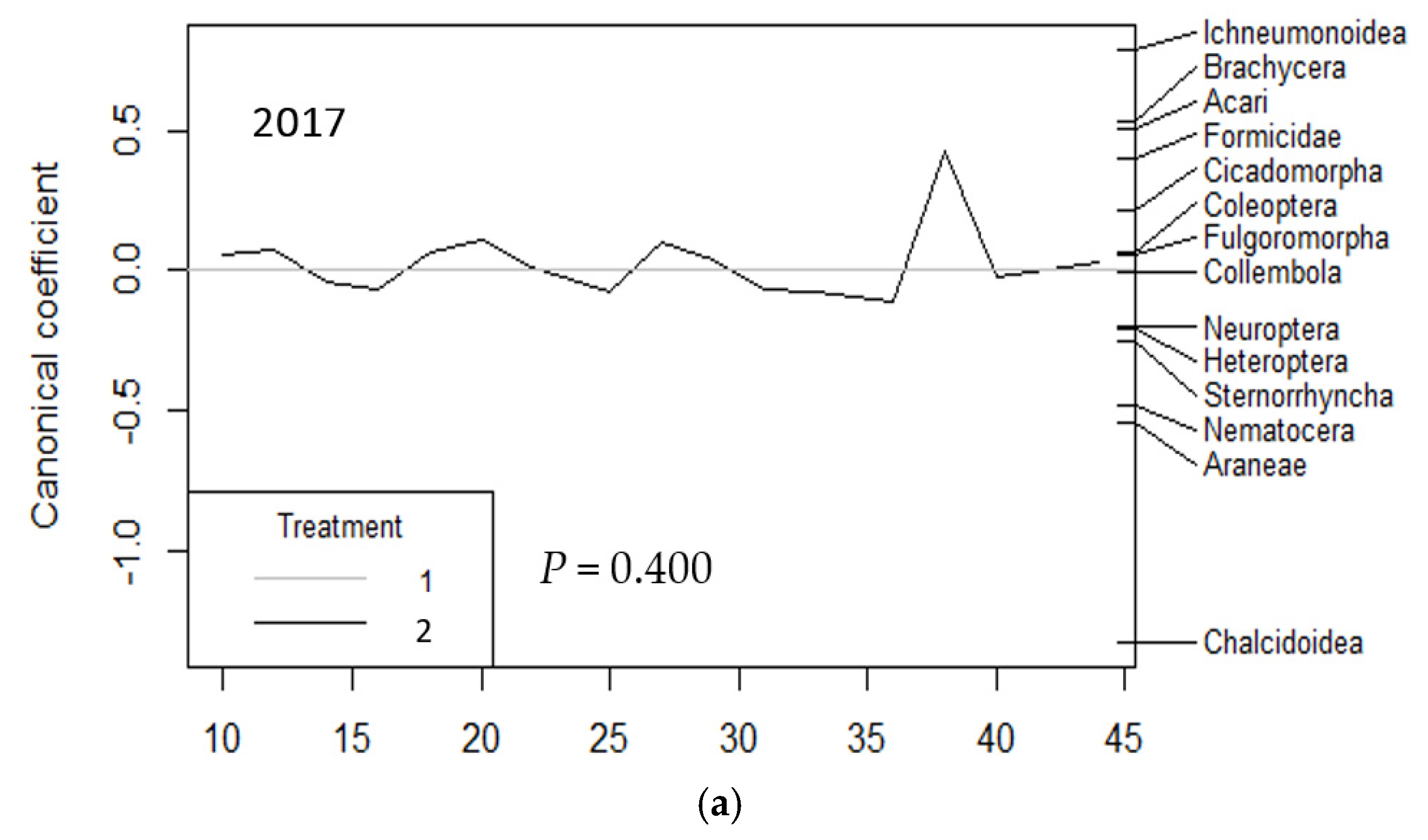
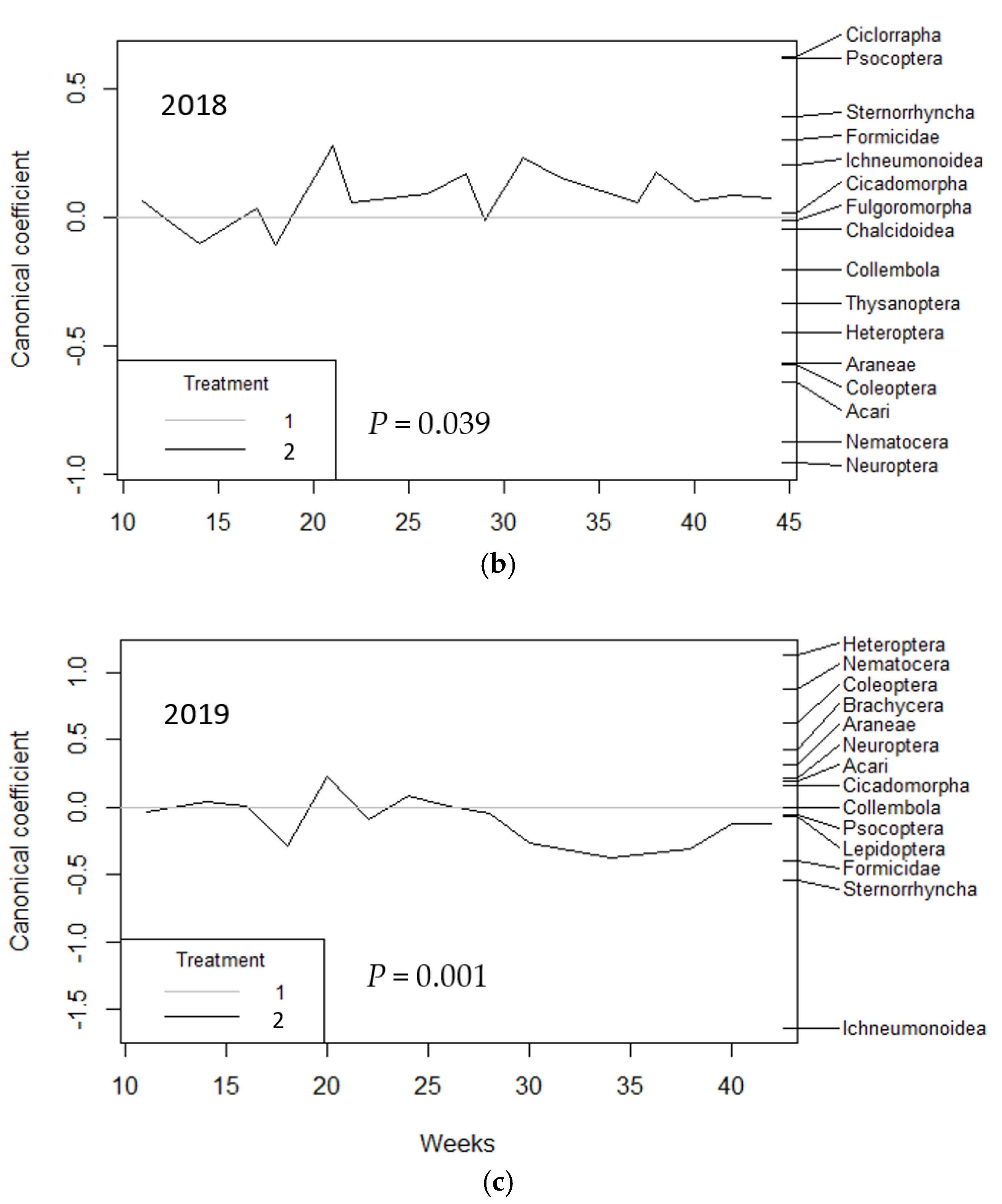
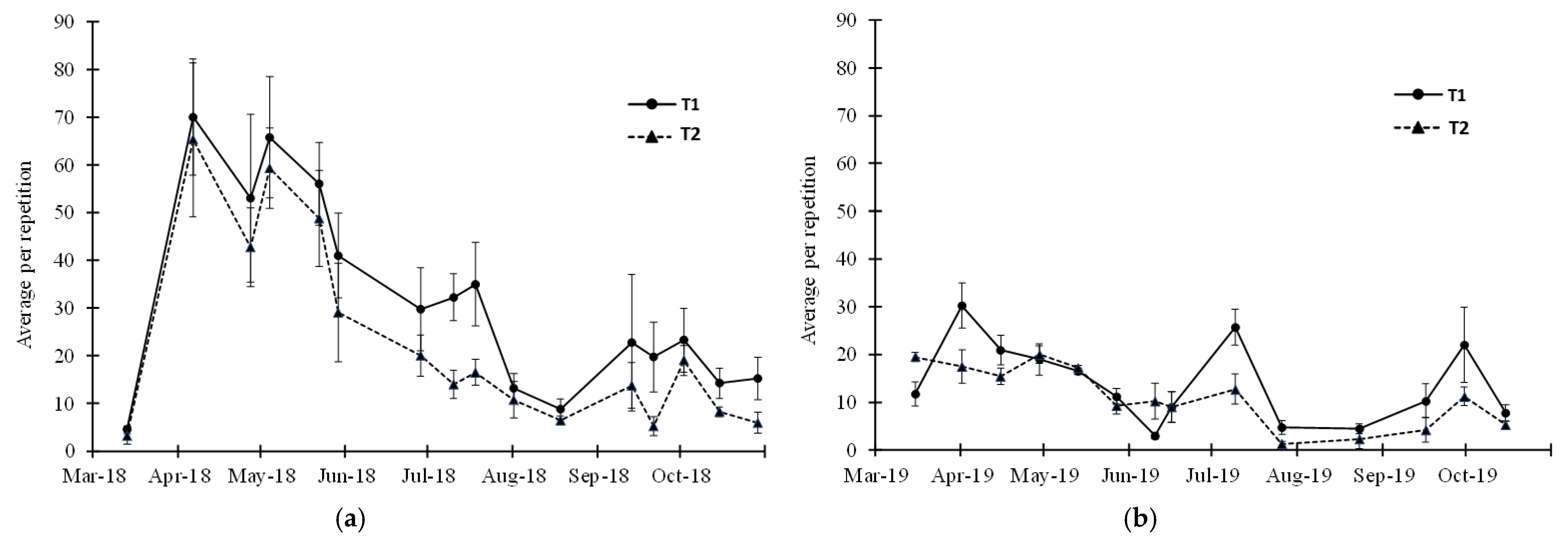
3.1. Vacuum Sampling

There were no statistical differences in the total arthropods aspired in both treatments in 2017 (F = 0.24; df = 1, 6; p = 0.640). In the other two years, there were significant differences between the irrigation treatments in the total arthropods aspired in 2018 (F = 10.95; df = 1, 6; p = 0.016) and in 2019 (F = 8.70; df = 1, 6; p = 0.026), and with more abundance in T1 (control) than in T2 (Confederation RDI). Taking together the three years of study, T1 had a significantly larger arthropod population than T2 (F = 15.6; df = 1, 18; p = 0.001). Results in Table 1 (significance) and

Table 2. Average per day and repetition (±SE) of the arthropods recuperated using the vacuum sampling method for the three years of study. Both treatments T1 and T2 had four plots (repetitions) each.

	2017		2018		2019		Total 1
	T1	T2	T1	T2	T1	T2
Arachnida	3.44 ± 0.58	4.14 ± 0.92	2.25 ± 0.37	1.80 ± 0.33	1.48 ± 0.31	1.00 ± 0.23	883
Araneae	1.14 ± 0.17	1.02 ± 0.17	1.52 ± 0.38	1.16 ± 0.25	0.91 * ± 0.16	0.61 * ± 0.18	394
Acari	2.30 ± 0.49	3.13 ± 0.83	0.73 ± 0.30	0.64 ± 0.31	0.57 ± 0.22	0.39 ± 0.20	489
Collembola	0.86 ± 0.41	0.59 ± 0.23	1.64 ± 0.71	1.58 ± 0.73	0.16 ± 0.09	0.27 ± 0.14	323
Coleoptera	0.44 ± 0.09	0.20 ± 0.06	0.81 ± 0.16	0.59 ± 0.12	0.88 ± 0.21	0.68 ± 0.20	218
Diptera	18.56 ± 2.27	16.66 ± 1.75	33.16 ± 3.27	24.36 ± 2.94	15.50 ± 1.45	12.05 ± 1.09	7491
Nematocera	15.91 ± 1.78	13.42 ± 1.50	31.53 * ± 3.17	23.02 * ± 2.85	14.05 ± 1.35	11.09 ± 0.97	6794
Brachycera	2.66 ± 0.72	3.23 ± 0.78	1.16 ± 0.18	1.27 ± 0.23	1.45 ± 0.2	0.96 ± 0.23	697
Hemiptera	8.25 ± 1.1	7.20 ± 0.9	8.08 ± 2.0	7.81 ± 1.7	6.34 ± 1.2	4.14 ± 1.02	2591
Heteroptera	6.41 ± 0.9	5.81 ± 0.8	7.09 ± 2.0	6.44 ± 1.7	5.36 ± 1.1	2.98 ± 0.89	2126
Cicadomorph	0.19 ± 0.0	0.19 ± 0.0	0.33 ± 0.1	0.28 ± 0.0	0.25 ± 0.0	0.14 ± 0.05	88
Fulgoromorpha	0.44 ± 0.30	0.13 ± 0.07	0.03 ± 0.02	0.00 ± 0.00	0.02 ± 0.02	0.00 ± 0.00	42
Sternorryncha	1.09 ± 0.24	0.83 ± 0.16	0.63 ± 0.12	1.09 ± 0.21	0.68 * ± 0.20	1.02 * ± 0.23	335
Hymenoptera	4.38 ± 0.42	4.28 ± 0.48	4.34 ± 0.74	3.95 ± 0.67	2.68 ± 0.54	2.93 ± 0.41	1399
Chalcidoidea	2.70 ± 0.39	2.63 ± 0.43	1.64 ± 0.42	0.66 ± 0.13	0.0 ± 0.0	0.07 ± 0.03	492
Ichneumonoidea	0.52 ± 0.10	0.63 ± 0.17	0.30 ± 0.11	0.42 ± 0.13	1.89 * ± 0.39	2.30 * ± 0.36	354
Formicidae	1.13 ± 0.21	0.94 ± 0.17	0.77 ± 0.26	0.75 ± 0.22	0.79 ± 0.22	0.55 ± 0.17	304
Other	0.02 ± 0.02	0.09 ± 0.04	1.64 ± 0.63	2.13 ± 0.64			249
Lepidoptera	0.22 ± 0.09	0.06 ± 0.03	0.25 ± 0.07	0.20 ± 0.08	0.18 ± 0.08	0.23 ± 0.11	70
Neuroptera	0.63 ± 0.15	0.69 ± 0.13	1.61 ± 0.54	1.00 ± 0.35	0.55 ± 0.16	0.57 ± 0.18	313
Psocoptera	0.17 ± 0.08	0.17 ± 0.06	0.72 ± 0.37	0.89 ± 0.38	0.52 ± 0.30	0.41 ± 0.19	177
Thysanoptera	0.13 ± 0.05	0.09 ± 0.04	1.06 ± 0.73	0.59 ± 0.43	0.02 ± 0.02	0.02 ± 0.02	122
Total	37.00 ± 3.33	33.98 ± 2.24	53.92 * ± 4.06	42.78 * ± 3.83	28.30 * ± 1.76	22.34 * ± 1.45	13587

Insect orders and other higher taxon are in bold. ¹ Calculated considering the number of sampling dates in each year: 16, 16, and 14 samples. * Significant differences between both treatments in each year.

(arthropod abundance), and more statistical outputs are presented in

Table A3. Results of the repeated-measures ANOVA for the three years of study showing the F statistics of the irrigation treatment (Tr) and interaction Treatment × Sampling Date (Tr × SD) for the most important variables registered in the visual and vacuum sampling methods for 2017 to 2019.

VACUUM	2017		2018		2019		2017 to 2019
	Tr	Tr × SD	Tr	Tr × SD	Tr	Tr × SD	Tr	Y	Tr × Y
Araneae	0.40	1.47 (4.5, 27.2)	1.0	1.70 (4.0, 24.1)	12.03	1.0 (4.4, 26.4)	6.31	2.90	1.03
Acari	0.48	0.52 (3.2, 19.2)	0.01	3.12 (2.4, 14.2)	1.03	2.2 (3.0, 17.9)	0.04	30.6	0.81
Collembola	0.33	3.70 (2.7, 16.2)	<0.01	0.80 (2.9, 17.4)	0.87	3.1 (3.8, 22.6)	0.35	7.11	0.04
Coleoptera	3.64	1.31 (4.0, 24.0)	2.20	0.83 (4.5, 26.7)	1.66	1.06 (3.3, 19.8)	6.51	6.19	0.01
Nematocera	1.91	0.75 (4.2,25.3)	21.52	0.70 (3.7, 22.2)	5.02	2.69 (2.6, 15.6)	16.2	40.0	0.35
Brachycera	0.95	0.66 (3.4, 20.6)	0.04	1.35 (4.2, 25.2)	3.05	2.91 (3.0, 18.2)	0.22	10.3	2.07
Heteroptera	1.17	0.91 (3.9, 23.4)	0.04	2.24 (4.1, 24.5)	2.93	2.47 (3.2, 19.5)	3.26	2.71	1.67
Cicadomorpha	0.05	1.46 (3.2, 19.2)	<0.01	2.24 (3.1, 18.7)	1.19	1.05 (3.0, 17.8)	0.07	1.58	0.52
Fulgoromorpha	1.45	0.94 (1.4, 8.2)	3.0	<0.01 (1.0, 6.0)	--(2)		2.48	10.7	0.44
Sternorrhyncha	0.81	0.78 (4.1, 24.6)	1.48	0.99 (3.4, 20.3)	7.43	2.18 (4.5, 27.2)	1.11	0.11	2.39
Chalcidoidea	0.49	2.39 (3.7, 22.4)	0.37	0.49 (3.9, 23.4)	--(2)		4.30	56.0	1.05
Ichneumonoidea	0.001	4.25 (3.7, 22.0)	0.80	0.88 (2.4, 14.1)	6.59	6.87 (3.3, 19.7)	4.02	88.2	3.41
Formicidae	0.13	0.64 (4.2, 25.1)	0.06	4.31 (2.9, 17.4)	1.20	3.06 (3.2, 19.0)	0.03	2.99	0.19
Other Hymenoptera	--(2)		0.16	2.26 (2.0, 12.1)	--(1)
Neuroptera	0.54	0.55 (3.9, 23.2)	3.01	1.92 (3.8, 22.6)	<0.01	1.90 (4.3, 25.6)	0.81	3.70	1.41
Psocoptera	--(2)		2.13	2.10 (3.1, 18.4)	0.01	1.08 (2.9, 17.5)	0.06	3.22	0.16
Thysanoptera	--(2)		1.54	0.77 (2.3, 13.9)	--(2)
Total arthropods	0.24	0.46 (3.8, 23.1)	10.95	0.39 (3.4, 20.5)	8.70	3.94 (3.9, 23.4)	15.6	49.5	3.42
VISUAL
Euphyllura (fl+sh)			2.39	1.30 (3.1, 24.7)
Euphyllura (fl)	0.37	0.04 (1, 8)	--(2)		0.14	0.33 (1.0, 3.0)	1.85	24.1	1.90
Euphyllura (sh)	--(1)		--(2)		<0.01	<0.01 (1.7, 13.8)
Lepidoptera	2.13	0.85 (3.4, 27)	16.7	1.58 (4.8, 38.2)	2.27	2.48 (2.9, 22.8)	14.0	61.3	11.9
Feeding spots (a)	1.50	0.57 (4.2, 34)	0.22	1.19 (4.2, 25.4)	0.14	0.89 (4.1, 24.4)	1.26	15.6	0.74
Feeding spots (b)	--(1)		9.91	0.92 (5.0, 40.1)	0.03	2.11 (3.9, 31.3)	4.56	49.8	4.06
Heteroptera	--(2)		0.29	1.49 (3.6, 29.1)	4.68	0.78 (2.4, 19.1)	2.28	4.46	1.82
Neuroptera	--(2)		0.07	0.74 (3.6, 28.8)	0.67	1.32 (3.4, 27.2)	0.81	9.20	0.03
Eriophyidae	0,16	0.63 (5, 38.4)	26.44	2.8 (4.7, 37.6)	17.20	2.22 (5.1, 41.1)	5.31	9.77	1.51
Phytoseiidae	--(2)		0.38	1.58 (3.6, 28.8)	--(2)
Other arthropods	1.05	0.51 (4.6, 36.6)	--(2)		--(2)
Venturia	0.07	1.19 (4.8, 38)	0.12	1.06 (1.9, 15.1)	0.06	1.99 (3.0, 23.8)	0.01	43.1	0.07

‘fl’ and ‘sh’ means ‘flowers’ and ‘shoots’, respectively; “Feeding spots (a)” indicates the proportion of leaves with the presence of feeding spots, “Feeding spots (b)” indicates the proportion of a leaf surface with feeding spots. The Euphyllura data were pooled together for the analysis of the three years (2017–2019). Degrees of freedom for the F statistics of Treatment (Tr) in the visual sampling: 1, 8; degrees of freedom for the F statistics of Treatment (Tr) in the vacuum sampling: 1, 6; degrees of freedom for the F statistics of Treatment × Sampling Date (Tr × SD), both in visual and vacuum sampling: between the brackets after applying the Greenhouse–Geisser’s degree of freedom correction. Degrees of freedom for the analysis of all three years together: visual (1, 42 (Treatment); 2, 42 (Year, and Year × Treatment) and vacuum (1, 18 (Treatment); 2, 18 (Year, and Year × Treatment)) sampling, except when there are only two years in the analysis. ⁽¹⁾ Not registered. ⁽²⁾ Not calculated due to the very low numbers of individuals.

(Appendix B).

Diptera Nematocera was the most abundant arthropod group in the aspiration sampling with 6794 individuals (Table 2). They presented significant differences between treatments only in 2018 (F = 21.52; df = 1, 6; p = 0.004). Nevertheless, considering all three years together, T1 had a significantly larger Nematocera population than T2 (F = 16.2; df = 1, 18; p = 0.001). Diptera Brachycera had much less individuals, and there was no statistical difference between treatments in all three years taken together or separately. Results are in Table 1 (significance) and Table 2 (arthropod abundance), and more statistical outputs are presented in Table A3 (Appendix B).

Hemiptera Heteroptera was the second-most abundant arthropod group, with 2126 individuals, but no significant differences were found between treatments for all three years taken together or separately, although there were larger populations in treatment T1 than in T2. One of the most frequently captured species was Brachynotocoris puncticornis Reuter (Heteroptera: Miridae). Results are in Table 1 (significance) and Table 2 (arthropod abundance), and more statistical outputs are presented in Table A3 (Appendix B).

Hymenoptera was another arthropod group well represented in the different groups observed (1399 individuals). Neuroptera is an important group for its role in biological control of several olive pests, and it appeared constantly in the three years, but no differences between irrigation treatments were observed (F = 0.81; df = 1, 6; p = 0.381). Other secondary groups showed significant differences between treatments, such as Araneae—significantly greater in T1 than in T2 for the three years (F = 6.31; df = 1, 18; p = 0.022)—and Coleoptera (F = 6.51; df = 1, 18; p= 0.020, analysis of the three years)—with populations in T1 significantly greater than in T2. Sternorrhyncha and Ichneumonoidea showed no differences between treatments in the analysis of the three years together, although they were significantly more abundant in T2 than in T1 only in 2019. However, their numbers were low and did not impact the total very much. Results are in Table 1 (significance) and Table 2 (arthropod abundance), and more statistical outputs are presented in Table A3 (Appendix B).

The PRC of vacuum sampling showed no differences between treatments in 2017 (p = 0.400, Figure 1a), but the treatments were significantly different in 2018 (p = 0.039, Figure 1b) and 2019 (p = 0.001, Figure 1c), confirming the results of the ANOVA analysis. Diptera Nematocera and Neuroptera (in 2018, Figure 1b) both have high negative weights (in the vertical right axis) and are of opposite signs to the canonical coefficient of T2, indicating that, in general, their populations were larger in T1 than in T2. Ichneumonoidea (in 2019, Figure 1c) also have a high negative weight and are of equal sign to that of the canonical coefficient of T2, thus indicating that their populations were higher in T2 than in T1.

As seen before, the total arthropods were significantly more abundant in T1 than in T2 in 2018 and 2019 (Table 1, vacuum). In both years, in general, T1 showed a larger population, although with a similar pattern than T2 (Figure 2a,b), with a peak at the beginning of the season. Only in 2019 there was a significant effect for Treatment × sampling date (F = 3.94; df = 3.9, 23.4; p = 0.014, Table 1, Table A3), especially at the end of the season, when total arthropods were more abundant in T1.

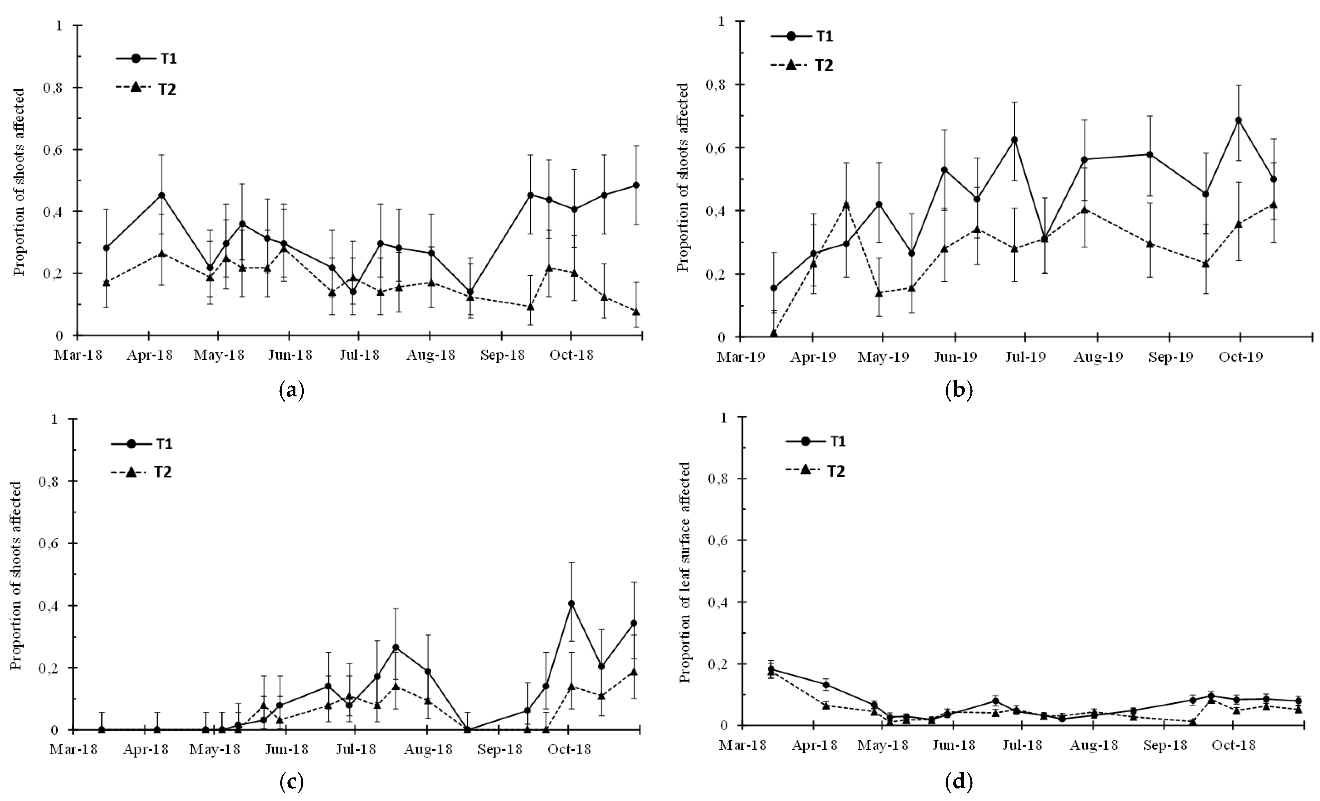
3.2. Visual Sampling

There was no significative response in 2017 due to the irrigation treatments with visual observations (Table 1). In 2018 and 2019, the presence of Eriophyidae (Trombidiformes) damage was significantly higher in T1 (control) than in T2 (Confederation RDI) (F = 26.44; df = 1, 8; p = 0.001 in 2018, and F = 17.20; df = 1, 8; p = 0.003 in 2019), and it was also significant when the three years were analyzed together (F = 5.31; df = 1, 42; p = 0.026), with T1 being more damaged than T2. Shoot damage produced by Lepidoptera, which includes Palpita unionalis Hübner (Lepidoptera: Crambidae) and Zelleria oleastrella (Milliere) (Lepidoptera: Yponomeutidae), was also significantly higher in T1 than in T2 (F = 16.7; df = 1, 8; p = 0.004) only in 2018, and when the three years were analyzed together, there were again significant differences in shoot damage (F = 14.0; df = 1, 42; p = 0.001, with T1 being more damaged than T2), although the interaction Treatment × Year was also very significant (F = 11.9; df = 2, 42; p = 0.001). The proportion of the foliar surface with feeding spots (Feeding spots (b)) was also significantly higher in T1 in 2018 (F = 9.91; df = 1, 8; p = 0.014), and again, when the three years were analyzed together, there were significant differences in foliar damage (F = 4.56; df = 1, 42; p = 0.042), with T1 having more feeding spots than T2). Results are in Table 1 (significance) and Table 2 (arthropod abundance), and more statistical outputs are presented in Table A3 (Appendix B).

The PRC of visual sampling showed no differences between treatments in 2017 (p = 0.786, Figure 3a), but in 2018 (p = 0.038, Figure 3b) and 2019 (p = 0.031, Figure 3c), statistically significant differences were found. The vertical right axis shows the weights of the different observations, their importance in the effect, and their response to the irrigation treatments. Eriophyidae (2018 and 2019, Figure 3b,c, respectively) and Lepidoptera (2018, Figure 3b) showed high negative values for their weights, opposite to the canonical coefficient of treatment T2 in the second part of the sampling period, which indicates that their presence was contrary to the evolution of treatment T2 and, thus, more abundant in T1.

Eriophyidae symptoms in the shoots were significantly more frequent in T1 than in T2 in 2018 and 2019 (Table 1, visual), and it was more evident in the latter part of the season (Figure 4a,b), when 50–60% of the shoots were affected in T1 whereas 10–40% of shoots were affected in T2, with the confidence intervals not overlapping. Lepidoptera presence and damage in shoots was significant in 2018 (Table 1, visual), and more evident in the middle and in the latter part of the season (Figure 4c), when 40% of the shoots were affected in T1 and 10–20% were affected in T2. The proportion of leaf surfaces with the presence of feeding spots was only significant in 2018 (Feeding spots (b), Table 1, visual), with more presence in T1 than in T2 (Figure 4d) throughout the season, although the percentage of the leaf surface affected was low and constant in both treatments.

Finally, no effect of the irrigation treatment was observed for the presence of peacock spots (V. oleaginea) on the leaves during the three years of study (F = 0.01; df = 1, 42; p = 0.948, Table 1, visual), although the method of observation was not exhaustive. More statistical outputs are presented in Table A3 (Appendix B).

4. Discussion

The general picture that can be drawn from this study is that more arthropods were present in T1 (control) than in T2 (Confederation RDI) and, more importantly, that some pests were also more abundant in T1 than in T2. Interestingly, the abundance of the most important groups of beneficial insects—Neuroptera, Ichneumonoidea, and Chalcidoidea—was not especially affected by the irrigation treatments, although Araneae was more abundant in the more watered treatment (T1). Water management and its effect on the arthropod community were also studied by Frampton et al. [14], although with different objectives, but they also found that irrigation increased the presence of arthropods in agricultural plots. Studies in woods also found that higher humidity (natural or not) increased in general arthropod abundance [15,16].

In our research, the irrigation treatments did not show any pattern in the first year of study (2017), but significant differences were found in the following two years (2018 and 2019). This is probably because the differential effect of irrigation was not evident in the first year of study.

For vacuum sampling, the most abundant group of arthropods was Nematocera, which was significantly more abundant in T1 than in T2 for all three years. Treatment T1 had more weeds in the tree rows and humidity in the soil, which could help to increase their presence [15,16]. The other groups were less abundant and of little influence in the general effect of irrigation, although there were significant differences between irrigation treatments for Araneae, Ichneumonoidea, and Sternorrhyncha in some years or even in the pooling of the years, such as for Araneae and Coleoptera; Collembola and Formicidae showed significant effects only in the interaction Treatment × Sampling Date.

The order Neuroptera—with the family Chrysopidae being the most relevant—is regarded as an important biological control agent for several pests in olive orchards [24]; in our research, it was reasonably present during the three years of study, but no effect of the irrigation treatment was observed in relation to its abundance.

Regarding visual sampling, Acari (Trombidiformes: Eriophyidae) was the most important group of arthropods observed for the symptoms produced in the shoots due to their feeding, which are clearly distinguishable and assigned to a group of gall mites or eriophyids species commonly present in the crop [39], of which Aceria oleae (Nal.) is the most important species. Some samples of leaves with these symptoms were taken to the laboratory on different occasions, and the presence of eriophyids was confirmed, although no species was positively identified. Eriophyid damage was significantly greater in T1 than in T2 in 2018 and 2019 (and for the combination of all three years). English-Loeb [12] also observed that Tetranychus urticae Koch (Trombidiformes: Tetranychidae) populations were most abundant on well-watered and on severely stressed Phaseolus vulgaris (bean) plants and least abundant on slight to moderately stressed plants. The presence of Lepidoptera—which comprises two species, P. unionalis and Z. oleastrella—larvae and damage on shoots was also significantly greater in T1 than in T2 in one year (2018). This behavior is similar to that observed for several experiments in which pot plants with low water stress (comparable with the T2 of our study) were less preferred than very stressed or well-watered plants by different lepidopteran pest larvae [17,18], a response that could be due to different components of the plant.

The presence of feeding spots on the leaves was also significantly greater in T1 than in T2 when taking all three years of study into account, although only in 2018 was relevant. Feeding spots were present on the leaves—mainly old leaves—and we hypothesized that they were produced by sucking feeding arthropods. The most abundant group with this type of feeding was Heteroptera—observed in the vacuum sampling data, mainly from the family Miridae, which has many phytophagous and zoophytophagous species [31] —but they were not easily observed during visual sampling, and there were no differences in its numbers between irrigation treatments, both in vacuum and visual sampling.

Some groups that were visually observed were also captured in vacuum sampling. Euphyllura olivina Costa (Hemiptera: Psyllidae)—included in the Sternorrhyncha suborder of the Hemiptera— is considered a secondary pest of olives in Spain [27]. Its nymphs feed on the shoots and inflorescences and are surrounded by a web of whitish threads, which makes them easily detectable. Vacuum sampling captured several adults and some nymphs of this species, but in both types of sampling, there were no significant differences between the irrigation treatments—except for 2019 in vacuum sampling—and their populations were low and of little significance.

There was almost no presence of Bactrocera oleae (Rossi) (Diptera: Tephritidae)—the most important pest of olive crop in Spain. Vacuum sampling is not the best method to study its populations, but fruit sampling in October 2017 and 2018 did not detected the presence of these larvae or any damage. The cultivar “Arbequina” is one of the least preferred by this pest [40], so this result is understandable. Another important olive pest in Spain is Prays oleae Bernard (Lepidoptera: Praydidae), which is easily detected when sampling inflorescences visually in April–May, but in the three years of this study, its presence was very low, and thus, it was not included in further analyses. The number of adults captured with the vacuum were also very low in the three years.

The interaction Treatment × Sampling Date was remarkable in Eriophyidae (visual sampling), and total arthropods (vacuum sampling) also showed a significant effect in the interaction (but only in 2019). In both cases, more damage/individuals were observed in T1 (compared with T2) at the end of the sampling period, when trees had a new sprouting period, especially in the most watered T1 treatment.

Visual sampling was more appropriate to scout specific pests of this crop—such as Eriophyidae, the Lepidopteran shoot feeders P. unionalis and Z. oleastrella, or symptoms of feeding activity on leaves. In this way, we were able to detect significant differences in 2018 and 2019 between treatments, as was represented in the PRC analysis and the repeated-measures ANOVA. More twigs and shoots were observed—not quantified—in the T1 treatment in spring and autumn, and it can be hypothesized that excess water produced more vigorous vegetation, where most of the detected pests proliferated. Another aspect that could influence this difference in population in both treatments is that moderate and intermittent drought—as in T2—can result in a surplus of carbohydrates (fewer carbohydrates are used for growth) becoming available for the synthesis of carbon-based defenses (terpenes and phenolics) [21]. A collateral benefit of less irrigation is the reduction in the vigor of these trees and, thus, the intensity of crop operations, such as mechanical pruning.

5. Conclusions

As a conclusion of this three-year study, although it was carried out only in one orchard, irrigation schemes with limited water use—e.g., treatment T2 (Confederation RDI) used in this study—can reduce the abundance of different pests in olive crops, especially of those who feed on the plants’ new sprouts. This is an important effect that should be considered in super-intensive olive orchards because it allows for not only the sustainable use of water but also more rational management of several pests in the crop, with collateral benefits in the cultural operations as well.

References

1. Junta de Andalucia Análisis de la Densidad en las Plantaciones de Olivar en Andalucia. Available online: https://www.juntadeandalucia.es/organismos/agriculturaganaderiapescaydesarrollosostenible/servicios/estadistica-cartografia/estudios-informes/detalle/184193.html (accessed on 27 April 2020).
2. Tribaldos Campos, J.; Tribaldos Campos, H. El Olivar en España: Tradicional, Intensivo y Superintensivo. Available online: https://www.agro.basf.es/es/Camposcopio/Secciones/Protección-y-sanidad/olivar-en-espana/ (accessed on 5 May 2021).
3. Moriana, A.; Pérez-López, D.; Gómez-Rico, A.; Salvador, M.; de los Desampadoros Salvador, M.; Olmedilla, N.; Ribas, F.; Fregapane, G. Irrigation scheduling for traditional, low-density olive orchards: Water relations and influence on oil characteristics. Agric. Water Manag. 2007, 87, 171–179. [Google Scholar] [CrossRef]
4. Fernández, J.E.; Perez-Martin, A.; Torres-Ruiz, J.M.; Cuevas, M.V.; Rodriguez-Dominguez, C.M.; Elsayed-Farag, S.; Morales-Sillero, A.; García, J.M.; Hernandez-Santana, V.; Diaz-Espejo, A. A regulated deficit irrigation strategy for hedgerow olive orchards with high plant density. Plant Soil 2013, 372, 279–295. [Google Scholar] [CrossRef] [Green Version]
5. Moriana, A.; Pérez-López, D.; Prieto, M.H.; Ramírez-Santa-Pau, M.; Pérez-Rodriguez, J.M. Midday stem water potential as a useful tool for estimating irrigation requirements in olive trees. Agric. Water Manag. 2012, 112, 43–54. [Google Scholar] [CrossRef]
6. Corell, M.; Martín-Palomo, M.J.; Pérez-López, D.; Centeno, A.; Girón, I.; Moreno, F.; Torrecillas, A.; Moriana, A. Approach for using trunk growth rate (TGR) in the irrigation scheduling of table olive orchards. Agric. Water Manag. 2017, 192, 12–20. [Google Scholar] [CrossRef]
7. Morales, F. Sustainable water use: Irrigation strategies in traditional Mediterranean and emerging crops. Agric. Water Manag. 2019, 217, 57–59. [Google Scholar] [CrossRef]
8. Galindo, A.; Collado-González, J.; Griñán, I.; Corell, M.; Centeno, A.; Martín-Palomo, M.J.; Girón, I.F.; Rodríguez, P.; Cruz, Z.N.; Memmi, H.; et al. Deficit irrigation and emerging fruit crops as a strategy to save water in Mediterranean semiarid agrosystems. Agric. Water Manag. 2018, 202, 311–324. [Google Scholar] [CrossRef]
9. Giorgi, F.; Lionello, P. Climate change projections for the Mediterranean region. Glob. Planet. Chang. 2008, 63, 90–104. [Google Scholar] [CrossRef]
10. Hodson, A.K.; Lampinen, B.D. Effects of cultivar and leaf traits on the abundance of Pacific spider mites in almond orchards. Arthropod-Plant. Interact. 2018, 13, 453–463. [Google Scholar] [CrossRef]
11. Goldhamer, D.A.; Viveros, M.; Salinas, M. Regulated deficit irrigation in almonds: Effects of variations in applied water and stress timing on yield and yield components. Irrig. Sci. 2006, 24, 101–114. [Google Scholar] [CrossRef]
12. English-Loeb, G.M. Plant drought stress and outbreaks of spider mites: A field test. Ecology 1990, 71, 1401–1411. [Google Scholar] [CrossRef]
13. Sconiers, W.B.; Eubanks, M.D. Not all droughts are created equal? The effects of stress severity on insect herbivore abundance. Arthropod-Plant. Interact. 2017, 11, 45–60. [Google Scholar] [CrossRef]
14. Frampton, G.K.; Van Den Brink, P.J.; Gould, P.J.L. Effects of spring drought and irrigation on farmland arthropods in southern Britain. J. Appl. Ecol. 2000, 37, 865–883. [Google Scholar] [CrossRef]
15. Lensing, J.R.; Todd, S.; Wise, D.H. The impact of altered precipitation on spatial stratification and activity-densities of springtails (Collembola) and spiders (Araneae). Ecol. Entomol. 2005, 30, 194–200. [Google Scholar] [CrossRef]
16. Lindberg, N.; Engtsson, J.B.; Persson, T. Effects of experimental irrigation and drought on the composition and diversity of soil fauna in a coniferous stand. J. Appl. Ecol. 2002, 39, 924–936. [Google Scholar] [CrossRef]
17. Gutbrodt, B.; Dorn, S.; Mody, K. Drought stress affects constitutive but not induced herbivore resistance in apple plants. Arthropod-Plant. Interact. 2012, 6, 171–179. [Google Scholar] [CrossRef] [Green Version]
18. Mody, K.; Eichenberger, D.; Dorn, S. Stress magnitude matters: Different intensities of pulsed water stress produce non-monotonic resistance responses of host plants to insect herbivores. Ecol. Entomol. 2009, 34, 133–143. [Google Scholar] [CrossRef]
19. Weldegergis, B.T.; Zhu, F.; Poelman, E.H.; Dicke, M. Drought stress affects plant metabolites and herbivore preference but not host location by its parasitoids. Oecologia 2015, 177, 701–713. [Google Scholar] [CrossRef]
20. Tariq, M.; Wright, D.J.; Rossiter, J.T.; Staley, J.T. Aphids in a changing world: Testing the plant stress, plant vigour and pulsed stress hypotheses. Agric. For. Entomol. 2012, 14, 177–185. [Google Scholar] [CrossRef]
21. Gely, C.; Laurance, S.G.W.; Stork, N.E. How do herbivorous insects respond to drought stress in trees? Biol. Rev. 2020, 95, 434–448. [Google Scholar] [CrossRef]
22. Ângelo Rodrigues, M.; Coelho, V.; Arrobas, M.; Gouveia, E.; Raimundo, S.; Correia, C.M.; Bento, A. The effect of nitrogen fertilization on the incidence of olive fruit fly, olive leaf spot and olive anthracnose in two olive cultivars grown in rainfed conditions. Sci. Hortic. 2019, 256, 108658. [Google Scholar] [CrossRef] [Green Version]
23. Villa, M.; Santos, S.A.P.; Sousa, J.P.; Ferreira, A.; da Silva, P.M.; Patanita, I.; Ortega, M.; Pascual, S.; Pereira, J.A. Landscape composition and configuration affect the abundance of the olive moth (Prays oleae, Bernard) in olive groves. Agric. Ecosyst. Environ. 2020, 294, 106854. [Google Scholar] [CrossRef]
24. Porcel, M.; Ruano, F.; Cotes, B.; Pena, A.; Campos, M. Agricultural Management Systems Affect the Green Lacewing Community (Neuroptera: Chrysopidae) in Olive Orchards in Southern Spain. Environ. Entomol. 2013, 42, 97–106. [Google Scholar] [CrossRef] [Green Version]
25. Cardenas, M.; Pascual, F.; Campos, M.; Pekar, S. The Spider Assemblage of Olive Groves Under Three Management Systems. Environ. Entomol. 2015, 44, 509–518. [Google Scholar] [CrossRef] [PubMed]
26. Paredes, D.; Cayuela, L.; Gurr, G.M.; Campos, M. Is ground cover vegetation an effective biological control enhancement strategy against Olive Pests? PLoS ONE 2015, 10, e0117265. [Google Scholar] [CrossRef] [PubMed] [Green Version]
27. Martín-Gil, A.; Ruiz-Torres, M. Guía de Gestión Integrada de Plagas-Olivar; Ministerio de Agricultura, Pesca y Alimentacion: Madrid, Spain, 2014; ISBN 9788449113871. [Google Scholar]
28. Rius, X.; Lacarte, J.M. Enfermedades y Plagas. In La Revolución del Olivar: El Cultivo en Seto; Rius, X., Lacarte, J.M., Eds.; Ediciones Paraninfo: Barcelona, Spain, 2015; pp. 383–405. ISBN 9780646938646. [Google Scholar]
29. Agustí-Brisach, C.; Jiménez-Urbano, J.P.; del Carmen Raya, M.; López-Moral, A.; Trapero, A. Vascular fungi associated with branch dieback of olive in super-high-density systems in Southern Spain. Plant Dis. 2021, 105, 797–818. [Google Scholar] [CrossRef] [PubMed]
30. Barrientos, J.A. Bases Para un Curso Práctico de Etomología; Asociación Española de Entomología: Salamanca, Spain, 1988; ISBN 84-404-2417-5. [Google Scholar]
31. Chinery, M. Guía de Campo de Los Insectos de España y de Europa; Omega: Barcelona, Spain, 2005; ISBN 84-282-0469-1. [Google Scholar]
32. Van Den Brink, P.J.; Ter Braak, C.J.F.T. Principal response curves: Analysis of time-dependent multivariate responses of biological community to stress. Environ. Toxicol. Chem. 1999, 18, 138–148. [Google Scholar] [CrossRef]
33. Dively, G.P. Impact of Transgenic VIP3A × Cry1Ab Lepidopteran-resistant Field Corn on the Nontarget Arthropod Community. Environ. Entomol. 2005, 34, 1267–1291. [Google Scholar] [CrossRef]
34. Prasifka, J.R.; Hellmich, R.L.; Dively, G.P.; Lewis, L.C. Assessing the Effects of Pest Management on Nontarget Arthropods: The Influence of Plot Size and Isolation. Environ. Entomol. 2005, 34, 1181–1192. [Google Scholar] [CrossRef]
35. Whitehouse, M.E.A.; Wilson, L.J.; Fitt, G.P. A comparison of arthropod communities in transgenic Bt and conventional cotton in Australia. Environ. Entomol. 2005, 34, 1224–1241. [Google Scholar] [CrossRef]
36. Naranjo, S.E. Long-term assessment of the effects of transgenic Bt cotton on the abundance of nontarget arthropod natural enemies. Environ. Entomol. 2005, 34, 1193–1210. [Google Scholar] [CrossRef] [Green Version]
37. Auber, A.; Travers-Trolet, M.; Villanueva, M.C.; Ernande, B. A new application of principal response curves for summarizing abrupt and cyclic shifts of communities over space. Ecosphere 2017, 8, e02023. [Google Scholar] [CrossRef] [Green Version]
38. Perry, J.N. Statistical aspects of field experiments. In Methods in Ecological and Agricultural Entomology; Dent, D.R., Walton, M.P., Eds.; CAB International: Oxford, UK, 1997; pp. 171–202. ISBN 0851991327. [Google Scholar]
39. González, M.I.; Alvarado, M.; Durán, J.M.; De la Rosa, A.; Serrano, A. Los eriófidos (Acarina, Eriophidae) del olivar de la provincia de Sevilla. Problemática y control. Boletín Sanid. Veg. 2000, 26, 203–214. [Google Scholar]
40. Quesada-Moraga, E.; Santiago-Álvarez, C.; Cubero-González, S.; Casado-Mármol, G.; Ariza-Fernández, A.; Yousef, M. Field evaluation of the susceptibility of mill and table olive varieties to egg-laying of olive fly. J. Appl. Entomol. 2018, 142, 765–774. [Google Scholar] [CrossRef] [Green Version]
Figure 1. Principal response curves (PRC) of the most important arthropods taxa in the vacuum sampling for (a) 2017, (b) 2018, and (c) 2019. The p values denote the significance of treatment T2 (Confederation RDI), represented as a plotted line, relative to the control treatment T1 (control) over all dates based on an F-type permutation test. The taxonomic groups are showed in the right vertical axis with their weights, which have the same scale as the canonical coefficients on the left vertical axis.
Agronomy 11 01337 g001aAgronomy 11 01337 g001b
Figure 2. Evolution along time for the average population of the total arthropod found using vacuum sampling in the two irrigation treatments: (a) in 2018 and (b) in 2019. The solid line represents treatment T1 (control), and the dotted line represents treatment T2 (Confederation RDI). The vertical bars represent the standard error of the mean.
Agronomy 11 01337 g002
Figure 3. Principal response curves (PRC) of the most important arthropod taxa and disease registered in the visual sampling for (a) 2017, (b) 2018, and (c) 2019. The p values denote the significance of treatment T2 (Confederation RDI), represented as a plotted line, relative to treatment T1 (control) over all dates based on an F-type permutation test. Observation groups are shown on the right vertical axis with their weights, which have the same scale as the canonical coefficients on the left vertical axis; ‘fl’ and ‘sh’ means ‘flowers’ and ‘shoots’, respectively.
Agronomy 11 01337 g003
Figure 4. Evolution along time for the proportion of the most important observations made using visual sampling in the two irrigation treatments: (a) Eriophyidae in 2018, (b) Eriophyidae in 2019, (c) Palpita unionalis and Zelleria oleastrella in 2018, and (d) feeding spots on the leaf surface in 2018. The solid line represents treatment T1 (control), and the dotted line represents treatment T2 (Confederation RDI). The vertical bars represent the exact confidence interval of a proportion, except for in d), which represents the standard error of the proportion.
Agronomy 11 01337 g004