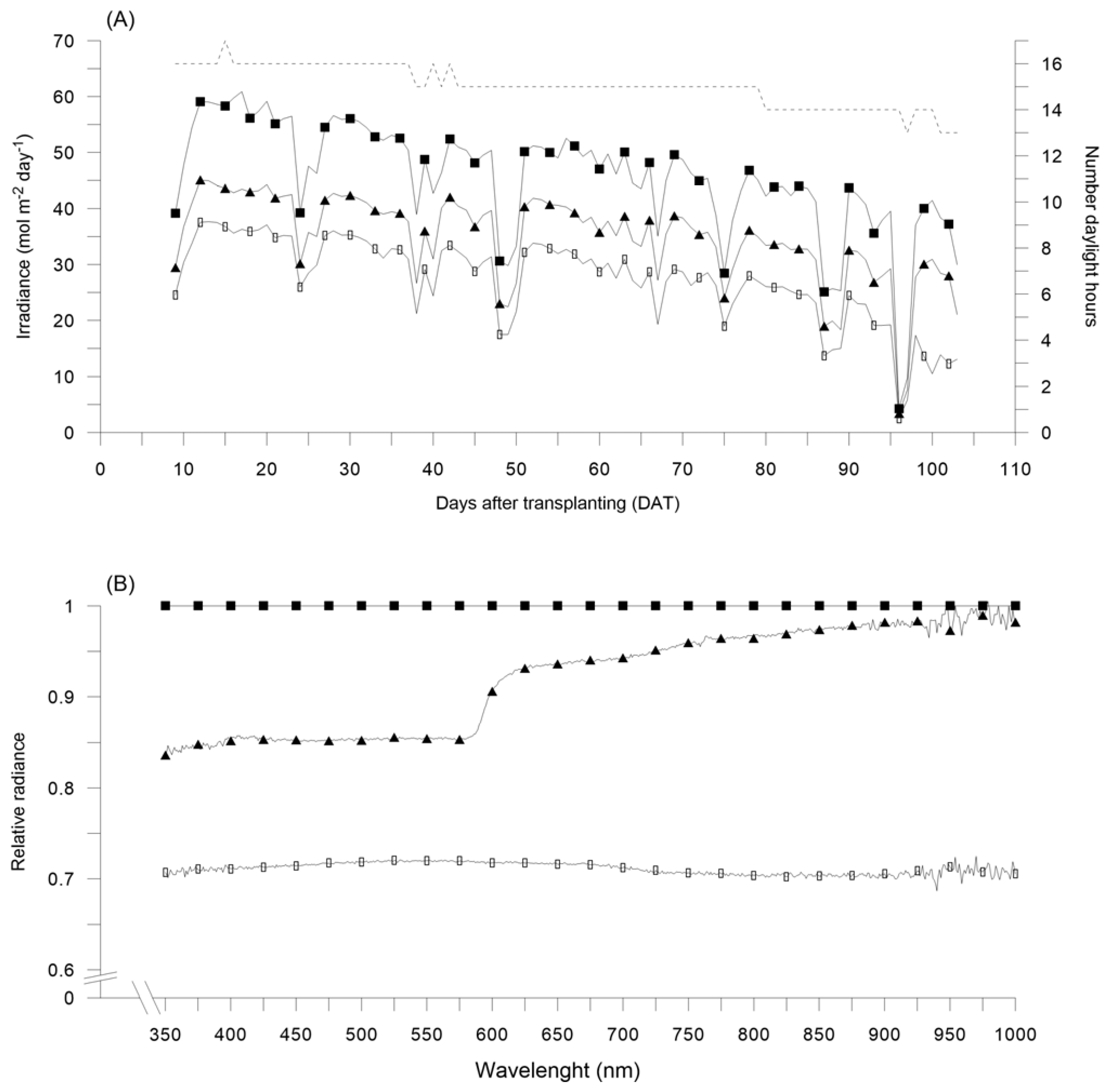
Article

Adaptive Responses to Nitrogen and Light Supplies of a Local Varieties of Sweet Pepper from the Abruzzo Region, Southern Italy

1
Faculty of Bioscience and Technology for Agriculture Food and Environment, Campus Universitario di Coste Sant’Agostino, University of Teramo, Via R. Balzarini 1, 64100 Teramo, Italy
2
Research Centre for Vegetable and Ornamental Crops, Council for Agricultural Research and Economics—CREA, Via Salaria 1, 63077 Monsampolo del Tronto, Italy
*
Author to whom correspondence should be addressed.
Agronomy 2021, 11(7), 1343; https://doi.org/10.3390/agronomy11071343
Submission received: 31 May 2021 / Revised: 25 June 2021 / Accepted: 28 June 2021 / Published: 30 June 2021

Abstract

:
Local varieties represent a heritage for plant biodiversity and, thanks to their resilience, are characterized by a better adaptation and rusticity to environmental variables. This work reports the morphological and physiological responses of a local ecotype of sweet pepper grown in Southern Italy, i.e., Altino, to N and light supplied at optimal and sub-optimal levels. In 2017, two open-field experiments were set up, comparing increasing N rates (0, 100 and 200 kg N ha−1, 0_N, 100_N and 200_N, respectively) and different percentages of shading and/or manipulations of the transmitted solar radiation, obtained through photoselective nets (red net, RN; black net, BN; unshaded Control). The unfertilized plants reduced growth (by 32% on average, at 83 days after transplanting, DAT), especially in terms of number of leaves, leaf area and effectiveness (chlorophyll content) of photosynthetic apparatus; no differences were recorded among fertilization treatments. On the other hand, the shading avoidance mechanisms resulted in higher biomass partitioned to leaves at the expense of sink organs, the building of more expanse (higher total leaf area) and thinner (higher specific leaf area and lower leaf-cuticular waxes) photosynthetic apparatus, and in a greater concentration of leaf pigments. The effects on yield and fruit quality of Altino ecotype deserve to be further explored.

1. Introduction

Capsicum annuum L. is one of the most cultivated and economically important vegetable species worldwide, being widespread on an area that exceeds 1.5 million hectares, including both spicy and sweet peppers [1,2,3]. The latter is mainly cultivated in the Mediterranean Basin where Italy represents one of the most important countries in the world, especially in south Regions [3].
Moreover, Italy, due to its geographical and historical compliance, includes a significant richness of cultivated biodiversity and landraces, which are important genetic reservoirs of useful genes. Among sweet pepper genotypes, the Altino ecotype is a typical niche of the horticultural product of the Abruzzo region (Southern Italy), and it is included in the traditional list of local products; fruits are harvested at maturity (red) and left to air-dry to obtain a powder to be used in many typical culinary dishes.
As a local variety, the Altino ecotype is characterized by good adaptation and rusticity and is prone to sustainable cultivation systems under low-input conditions [4], e.g., reduced the total use of agricultural chemicals, especially nitrogen (N) fertilization. In any case, N management must be calibrated based on the critical N curve and the N use efficiency to reduce N losses and environmental pollution [5]. Moreover, such ecotype could take advantage of some crop protection practices, such as the use of photoselective nets, finding a valid justification in the high added value of local productions (i.e., DOP, IGP, Slow Food praesidium). Netting, besides a significant improvement in terms of yield and post-harvest quality of many horticultural crops [6,7,8]—including sweet pepper [9]—can induce a moderate cooling effect useful in pest control [10] as well as protect fruits from sunburn damages [11] in prone vegetables, such as Altino ecotype.
In general, studies on the response of local varieties to agronomic techniques and environmental conditions are missing. Besides, it is essential to understand the mechanisms of adaptation of such genotypes both to support plant breeding for high-quality products and agronomic management under low-input environments, as well as to increase farming systems diffusion in marginal areas. N availability and the amount of photosynthetically active radiation (PAR) transmitted to the canopy are two of the major determinants affecting plant morphological, anatomical, and physiological responses. Nitrogen is, indeed, essential for normal growth and development, being an integral part of protein development and chloroplast structure [12]. Under low-N conditions, a decrease in C assimilation, resulting in a consequent decrease in the mesophyll cell surface area per unit leaf area, is observed [13]. Moreover, plants grown under low-light environments are taken to invest more biomass in leaves, at the expense of roots, to access the most limiting factor, i.e., radiation [14].
Taken into account such considerations, our study was based on the following assumptions: (i) N and light supply are the major determinants in crop growth and development; (ii) such growth factors can be easily modulated in open-field by manipulating agronomic practices under low-input systems to enhance yield and quality (harvest and post-harvest) of local productions; (iii) the study of plant responses to the growth environment is specie- and genotype-specific; and (iv) local varieties are among the less studied ones in terms of adaptive response to both environment and agronomic techniques.
Therefore, the objective of this study was to evaluate both the separate and combinate effects of light and N supplied at optimal and suboptimal levels, on growth, morphological, and physiological responses of Altino ecotype plants. To reduce the experimental error coming from the normal genetic variation occurring within the local population, the collection of Altino ecotype was previously subjected to 2 cycles of selection and self-fertilization, as is fully described in the Section 2.

2. Materials and Methods

2.1. Plant Materials

Seeds of red sweet pepper Capsicum annuum L. ecotype “Altino” were provided in 2015 by a keeper farmer located at Altino (CH), in the Abruzzo region (Central Italy). Despite pepper is considered an autogamous species, it can attract insects, and allogamy can reach up to 40% to 100% under favourable conditions [15]. As a consequence, the collection was initially characterized for its uniformity in terms of growth habitus, yield aptitude as well as fruits shape and size, and subjected to two cycles of phenotypic selection (2015 and 2016), purging phenotypes carrying “off-specific” traits, as detailed below.
During the first year, pepper plants—grown at the experimental field of the Research Centre for Vegetable and Ornamental Crops, Council for Agricultural Research and Economics (CREA-OF), located in Monsampolo del Tronto (AP) (latitude 42°52′59.1″ N, longitude 13°48′01.9″ E), in the coastal area of the Marche Region (Central Italy) from May to September 2015—was cultivated in an experimental field of 1600 m2. The crop was managed according to the typical pepper cultivation techniques; plants were grown in twin-rows with a spacing of 0.4 m between plants and rows, and 0.8 m between twin-rows. Plastic mulching was applied into the twin-rows, while a mechanical weeds control was performed between twin rows. Phenotypes (plants) were selected based on the keeper farmers’ local knowledge and the defective ones were excluded from the selection. Plants corresponding to the ideotype were self-fertilized under a net isolator and seeds were collected for the second phenotypic’ selection cycle, performed in 2016 in a second experimental field at the CREA-OF. Eleven pepper phenotypes were cultivated in about 10 m × 13 m plots, following the agronomic practices adopted in the previous year. As in 2015, the phenotypes (plants) corresponding to the ideotype (in terms of both plant and fruits morphological traits) were marked and self-fertilized to obtain pure seeds to be used in the “agronomic” experiments (see Section 2.2 and Section 2.3), carried out in 2017. As early as the second generation of self-fertilization was sufficiently stable for the typical characters indicated for the ideotype and two phenotypes (named as 97 and 99, see Figure S1), characterized by analogues and uniform morphological traits, were selected; the main measured morphological characteristics (weight, diameter, and length of the fruits when ripe) are shown in Table S1.

2.2. Site Description

In 2017 (from 15 May to 22 September), two experiments (named as Exp_1 and Exp_2) were carried out at the experimental fields of the CREA-OF (Monsampolo del Tronto), using seeds of the two phenotypes 97 and 99, for Exp_1 and Exp_2, respectively.
The location is characterized by a typical thermal-mediterranean climate, with winter temperatures that can fall below 0 °C, and summer temperatures that can rise above 40 °C. The rainfall is mainly concentrated between October and April. During the experimental period, meteorological data were recorded by a meteorological station situated ~600 m from the experimental field. The average temperature over the crop growing cycle was 22.0 °C, with peaks of 38.1 °C in the first decade of August; during the May—September period, the crop received 95.8 mm of rain.
Pepper was grown on soil previously hosting artichoke, with the main characteristics: 392 g kg1 sand, 367 g kg1 silt, 241 g kg1 clay, 1.50% organic matter, and 0.80 g kg1 total N (soil NO3-N and NH4-N = 11.90 and 1.36 mg kg1, respectively).

2.3. Experiments Description and Growing Conditions

In both Exp_1 and Exp_2, pepper seeds were sown on 15 May 2017 in a nursery substrate and maintained in the greenhouse, under controlled conditions. Plants were transplanted on 6 June 2017, as 22-days-old seedlings (4 leaf stage), in the open field in twin-rows with a spacing of 0.4 m between plants and rows, and 1.6 m between twin-rows. The distance between twin-rows was justified to ensure compliance with a sufficient edge area between experimental treatments, as detailed reported below.
Both experiments were arranged as a split-plot design with three replications, comparing three nitrogen fertilization rates (main treatment) and three shade conditions (secondary treatment), for a total of nine experimental treatments obtained from the N × Shade combinations.
The main treatments were established in an experimental area of about 17.4 m2 each, including a single pepper twin row and a total of 72 pepper plants. The three N fertilization rates consisted in a 0, 100 and 200 kg N ha−1 nutrition (named 0_N, 100_N and 200_N, respectively), obtained by applying Urea at 9 days after transplanting (DAT).
For each N treatments, subplots were obtained by splitting the total area in three sub-plots of 4.8 m2 (20 pepper plants; Figure S2). Shading conditions were accomplished using different coloured shading nets (Sh treatments: red net, RN; black net, BN) in addition to an unshaded control (Control), wrapped around 1.7 m-height tunnels, placed over the crop. To allow air circulation on the hottest days, tunnels were open at both ends. Each subplot consisted of a total of 20 pepper plants, grown in a single twin-row. Red and Black nets were provided by Agrintech S.r.l. (Iridium®Rosso and Monotex 30, respectively; Eboli, SA, Italy); the main environmental characteristics recorded under RN and BN with respect to Control are reported in Table S2.
Photosynthetically Active Radiation (PAR) intensity was measured with a PAR Photon Flux Sensor (Decagon Devices Inc., Pullman, WA, USA) placed above the vegetation and connected to a data logger (EM50 Data Collection System, Decagon Devices Inc., Pullman, WA, USA), at 15-min intervals starting from 9 DAT, till to crop harvest; the irradiance daily quantum input (DQI, mol m−2), as recorded during the pepper cycle, was reported in Figure 1A. The amount of shading (%) was determined by comparing the daily average PAR values of nets with the daily average PAR values of the Control treatment. Following Shahak et al. [16], the amount of scattered light in the PAR region was measured at noontime of clear days using an opaque disc, held to 30–40 cm above the PAR sensor and its percentage was then calculated as the ratio between not-direct light to total light. To obtain information about the absorbed and transmitted radiation by photo-selective nets, radiance under coloured films was measured with the HandHeld 2 Pro Portable Spectroradiometer (FieldSpec, ADS Inc., Boulder, CO, USA), which measures radiation in the visible and near-infrared (NIR) wavelengths from 325 to 1075 nm (±2 nm), using a reflective surface characterized by a certificated reflectivity of 99%. Measurements were taken, at noontime and within a few minutes of sunny days during the middle phases of the crop cycles, with (shaded treatments) and without (Control) coloured nets; relative radiance (as a mean value of four measurements, two for Exp_1 and two for Exp_2) of RN and BN with respect to Control is reported in Figure 1B.
Relative humidity and air temperatures under coloured nets were recorded by sensors of temperature and humidity connected to a data logger system (EM50 Data Collection System, Decagon Devices Inc., Pullman, WA, USA) (Table S2).
The fixed sensors for the in-continuum measurements of the environmental parameters under photo-selective nets were placed only in Exp_1, considering the use of the same-coloured nets among the two experiments.
Crop was fertilized with potassium and phosphorus during soil preparation, at the rate of 80 and 150 kg ha−1 of P2O5 and K2O, respectively. Black plastic mulch and the drip irrigation plastic tubing were placed on pepper twin-rows. Weeds were mechanically and manually controlled between twin-rows and on the rows, respectively. No insecticide treatment was carried out; when necessary, fungal diseases were treated with CUPROXAT® SDI (Nufarm Italy, Milano, Italy), at the dose of 2 L ha−1.

2.4. Growth Analysis, Morphological Traits, and N Determinations

In both Exp_1 and Exp_2 two plants per experimental unit (each sub-plot of 20 plants) were sampled at 21, 42 and 83 DAT. Sampled plants were separated into leaves, stems and reproductive organs (flowers at 21 DAT; flowers and green fruits at 42 DAT; green, ripening and red fruits at 83 DAT) dried with an oven at 70 °C, until constant weight (DW determination). Before drying, stem length (cm), stem diameter (mm), and number of leaves (num) was measured; leaf area (LA, cm2) was recorded after acquiring scanned leaves’ images with an image analysis software (ImageJ, National Institutes of Health, Bethesda, MD, USA). The specific leaf area (SLA, cm2 g−1) was then calculated.
Starting from organs DWs, leaf mass ratio (LMR), stem mass ratio (SMR) and reproductive organs mass ratio (RMR) were calculated as the ratios between leaf, stems and reproductive organs (flowers/fruits) to total DW, respectively.
Relative growth rate (RGR g g−1 DAT) was estimated applying the following equation:
RGR   = ( ln   M t   ln   M t 1 )   ( t     t 1 )
where Mt and Mt−1 represent the total dry biomass at time t and t − 1, respectively.
The leaf area ratio (LAR, cm2 g−1), that is the amount of leaf area a plant develops per unit total plant mass, was calculated as the ratio between leaf area and total plant biomass. The net assimilation rate (NAR, g cm−2 day−1), i.e., the net biomass gain expressed on leaf area basis, was calculated as follows:
NAR   = ( M t M t 1 )   ×   ( ln LA t ln   LA t 1 )   ( LA t LA t 1 )   ×   ( t     t 1 )
where LAt and LAt−1 represent the leaf area t and t − 1, respectively, while Mt and Mt−1 are previously described; time is expressed as DAT.
Dried sub-samples of pepper fruits (or flowers), stems and leaves were analyzed to determine their N concentration following the Kjeldahl digestion method; the analyses were performed in duplicate at 0, 21, 42 and 83 DAT. At 83 DAT, analysis was also performed on separated green, ripening and mature fruits.

2.5. Physiological Parameters

The soil-plant analysis development (SPAD) and leaf temperature (TIR) assessments were performed on both Exp_1 and Exp_2 during all the crop cycle at 15, 31, 41, 52, 64, 91, and 104 DAT.
The SPAD 502 plus portable chlorophyll meter (Konica Minolta, Inc., Tokyo, Japan) was used to estimate chlorophyll content in five fully expanded and same sun-oriented leaves of three plants per experimental unit.
Leaf temperature (TIR) was recorded with a portable infrared thermometer (Everest Interscience Inc., Tucson, AZ, USA), at 20 cm from the leaf surface (uppermost leaf of three plants per experimental unit).
Canopy reflectance was measured with a HandHeld 2 Pro Portable FieldSpec Spectroradiometer (ADS Inc., Boulder, CO, USA) on three plants per experimental unit, at 15, 41, and 91 DAT. The instrument measures spectra over a spectral range of 325–1075 nm. To minimize the effects of the sun’s position, the reflectance measurements were taken within 1 h, near solar noon. Some important literature vegetation indices was then calculated: normalized difference vegetation index (NDVI; [17]); green normalized difference vegetation index (GNDVI; [18]); modified chlorophyll absorption ratio index (MCARI; [19]); optimized soil-adjusted vegetation index (OSAVI; [20]); and water index (WI; [21]).

2.6. Analytical Determination

Leaf pigment concentrations were determined during the vegetative/early reproductive phase of the pepper growing cycle at 21 and 42 DAT. Starting from sampled materials (as described in Section 2.4), we selected three fully expanded leaves per plant, characterized by the same position on the plant (i.e., primary, or secondary branches) as well as the same growth stage. From these sub-samples, the foliar pigments, named chlorophyll (Chla), Chlb, and carotenoids (Car) were determined following the method described by Lichtenthaler and Buschmann [22]. The results were expressed in µg g1 of fresh weight (FW).
Cuticular waxes were determined by gravimetric analysis, as previously described [23]. Two uppermost fully expanded leaves per sampled plant was collected at 21 and 42 DAT. The amount of wax was expressed against leaf area (both leaves’ surfaces), as determined by acquiring scanned leaves’ images with an image analysis software (ImageJ, National Institutes of Health, Bethesda, MD, USA).

2.7. Statistical Analysis

A three-way analysis of variance (ANOVA) was applied to test (F-test) the effects of the experiment (Exp) and treatments (N fertilization rates: N_rates; Sh levels: Sh_lev). Since no significant effects of ‘Exp’ or ‘Exp × N_rates’ or ‘Exp × Sh_lev’ or ‘Exp × N_rates × Sh_lev’ interactions were detected, we have reported in Tables and Figures only the main effects of treatments or their interaction. ANOVA assumptions were tested through graphical methods. The statistical analyses were performed using R software [24].

3. Results

3.1. Growth Conditions

The application of two photoselective nets sharply affected both the amount and quality of the radiation transmitted to the canopy with respect to Control. Figure 1A shows the evolution of daily values of DQI for the three light treatments: BN gave the lowest values while Control the highest. The highest PAR reduction was observed for BN (40.4% of shading), followed by RN (23.8%) with the former showing also the lowest relative amounts of scattered PAR (12.1% vs. 15.4% BN and RN, respectively; Table S2). BN reduced uniformly the radiance values, with no remarkable differences between wavelengths; conversely, RN showed a greater absorption around 350–550 nm (violet-green region) with respect to the other spectral bands (Figure 2).
Little differences were also recorded in terms of day-night thermal excursion, with RN showing the highest values (10.7 °C; Table S2), as well as of RH (58.4%, 57.8%, and 59.6%, for Control, RN, and BN, respectively; Table S2). However, these differences can be considered negligible.

3.2. Growth Analysis and Morphological Parameters

Vegetative and reproductive pepper’ organs DWs and total DWs responses to N fertilization rates and Sh conditions are reported in Table 1. At 21 DAT, N availability was the most determining factor influencing plant growth; not significant differences between 100_N and 200_N were recorded. Similar behaviours were observed at both 42 and 83 DAT. The effect of Sh conditions was pretty unclear and was mainly significant at 42 DAT, with RN showing the higher DWs values; conversely, BN showed the significantly highest leaves DW at 83 DAT (Table 1).
In Figure 2 is reported the biomass allocation among vegetative and reproductive organs during the pepper crop cycle.
As expected, during the crop cycle the biomass allocated to vegetative organs (i.e., leaves and stems) basically decreased to the advantage of newly produced biomass allocated to fruits. However, the PAR transmitted to the canopy played a significant role in the biomass allocation process, especially in terms of LMR and ReMR (see the box in Figure 2). In particular, at 83 DAT, plants under BN showed significantly higher and lower values of LMR of ReMR respectively than RN and Control (LMR: 0.302 vs. 0.245 and 0.236 g g−1 DW for BN, RN and Control, respectively; ReMR: 0.632 vs. 0.689 and 0.702 g g−1 DW for BN, RN and Control, respectively) which recorded similar values (Figure 2).
Besides, N and light availability sharply affected the number of leaves per plant as well as the total and single leaf area (Table 2; see from 42 DAT). In particular, the NumLf seemed to decrease at higher Sh intensity, while the highest LA and single LA values were generally recorded under BN at the highest fertilization rates, although significance varied among treatments and DAT (see Table 2). Interesting, RN, under 200 Kg N ha−1, induced LA and single LA values comparable with those obtained under BN. Despite such a trend, SLA significantly differed only in the middle phase of the pepper cycle, with BN showing the highest values, regardless of N doses (Table 2).
Under low-PAR availability, stem length increased up to 42 DAT (Table 3). On the other hand, Sh × N fertilization interaction seemed to significantly influence stem diameter at 42 and 83 DAT. In this case, the highest values were observed under shading for plants fertilized with 200 (or 100) kg N ha1 (Table 3).
RGR was not affected by treatments, NAR significantly reduced under limited PAR conditions while LAR increased (Table 4).

3.3. N Accumulation and Dynamics

The dynamics of leaf+stem N content per shoot (NLw), total N content per shoot (NTw), and leaf+stem N content per unit leaf area (NLa) during the pepper growing cycle are reported in Figure 3.
As expected, both NLw and NTw increased with fertilization rates; however, this increase was more pronounced under Control and RN treatments, especially in terms of NTw. Starting from the beginning of fruit formation (42 DAT), significantly increased the amount of N translocated to the growing fruits. Under the lowest N availability (0_N) shading stimulated N accumulation in harvested vegetative and reproductive organs (NLw: 1.19 g plant1 for BN vs. 0.80 g plant1, averaged over Control and RN; NTw: 3.37 g plant1 for BN vs. 2.71 g plant1, averaged over Control and RN). Conversely, in fertilized plants the amount of N translocated to fruits seemed to decrease in response to Sh conditions (83 DAT). Regardless of PAR availability, the amount of N directed to fruits was higher in N_200 rather than N_100 (Figure 3).
N fertilization induced also higher NLa values (Figure 3). An unclear pattern emerged in response to Sh or ShxN dose interaction. At 83 DAT, BN showed the highest NLa values at 0_N and the lowest at 200_N (Figure 3; 0_N: 0.79, 0.73, and 0.82 g cm2 for Control, RN, and BN, respectively; 100_N: 0.92, 0.90, and 0.90 g cm2 for Control, RN, and BN, respectively; 200_N: 0.93, 0.78, and 0.67 g cm2 for Control, RN, and BN, respectively).
N concentration data partially confirmed those observed in terms of N content (Figure 4). N fertilization sharply contributed to differences in terms of N concentration in fruits, whit higher values in 200_N and without significant differences among Sh conditions (Figure 4).

3.4. Physiological Adjustments to Growth Conditions

N fertilization as well as Sh conditions significantly affected SPAD values (see the box in Figure 5); such differences tended to decrease later in the crop cycle. In general, N fertilization enhanced the estimated chlorophyll content in pepper leaves (52.9, 56.1, and 56.3 for 0_N, 100_N, and 200_N, respectively, averaged over Sh and DAT), while the higher SPAD values were assured by fully-light conditions (56.6, 54.0, and 54.7 for Control, RN, and BN, respectively, averaged over N rates and DAT).
SPAD results were partially confirmed by the Chl concentration in pepper leaves, recorded only during the early stages of the crop growing cycle (Table 5). Indeed, at 21 DAT, Chl content increased as N availability and Sh levels increased. However, these differences disappeared as the cycle went on (Table 5).
Vegetation indices from canopy reflectance are reported in Table 6. The first four VIs i.e., NDVI, GNDVI, MCARI, and OSAVI, are somehow linked to crop physiology, green biomass and Chl content and their values describe an unclear pattern. Fact_2 seemed to mostly affect canopy reflectance, especially in the middle phases of the crop cycle, and in the case of MCARI (with no significant differences between RN and BN), OSAVI and NDVI (with BN showing significantly higher values than RN and Control); on the other hand, full-light assured the highest GNDVI values (Table 6).
WI, as an indicator of crop water status, was influenced by the photoselective nets, starting from 41 DAT; the lowest values were observed under shaded conditions (Table 6).
Regardless of N fertilization rates, Sh induced progressive lower (as the level of shading progresses) TIR values during all the crop growing cycle (29.0, 27.8, and 26.5 °C for Control, RN, and BN, respectively, averaged over N rates and DAT; Figure 6).
Light and N availabilities affected cuticular wax production in pepper leaves, in the early stages of the crop cycle (i.e., 21 and 42 DAT; Table 7). In particular, the amount of wax per unit leaf area decreased in response to N fertilization and progressive shading conditions. At 42 DAT, significantly higher values were observed for 0_N and Control Table 7.

4. Discussion

Adaptive responses of plants to the environment are accomplished through a broad range of significant modifications of important growth, morphological and physiological parameters [13].
In this study, the modification of N and light availability substantially affected the growth and resource allocation patterns of pepper plants. The effects of nitrogen availability on crop growth were clear and 100 kg N ha−1 resulted enough to guarantee good growth performances. Conversely, the influence of photoselective nets on dry biomass was quite undefined. Although the rate of dry mass accumulation is directly related to PAR availability [25], RN application resulted to stimulate biomass production, as already reported in previous studies on other horticultural crops [6,16,26], including sweet pepper [27]. This could be attributed to the mixture of filtered and unfiltered light passing through the red photoselective net [28] and to the higher light scattering (diffuse light) [6,29] than black net, which showed a sharp reduction of transmitted PAR (shading percentage about double than RN). In addition, while BN merely induced a reduction of light intensity [30], RN produces a spectral modification, with a significantly lower B:R (blue:red) and B:FR (blue:far red) ratios than Control and BN (B:R ratio: 0.889 ± 0.001, 0.970 ± 0.006, and 0.997 ± 0.002 for RN, BN, and Control, respectively; B:FR ratio: 1.051 ± 0.003, 1.192 ± 0.010, and 1.226 ± 0.003 for RN, BN, and Control, respectively).
However, as adaptive responses to the reduction of PAR availability pepper plants of Altino genotype adjusted their morphology and anatomy to capture more light through increasing total and single leaf surface and lowering leaf thickness (higher SLA values), especially at the highest N dose, as previously observed in other sweet pepper genotypes [31,32,33] as well as horticultural species [25,34,35,36]. These results confirmed that the role of N was crucial in stimulating the adaptation responses of the crop under abiotic stress circumstances, allowing pepper plants to build up to longer and larger stems [37]. Furthermore, according to the functional balance hypothesis [38], pepper plants coped with low-light conditions by relocating less assimilates to the sink organs (lower SMR and ReMR), reducing source activity (increasing of both LMR and LAR; [36]) and favouring the building-up of a more expanse and thinner photosynthetic apparatus (higher LA and SLA), characterized by a reduced rate of photosynthesis per unit leaf mass (i.e., low NAR; [39])—all shading avoidance mechanisms. Besides, leaf-cuticular wax contents to protect plants from high irradiation levels and UV-light [40], decreased. It can be assumed that the effects registered on leaves could be the same on pepper fruits. Considering the biological roles of cuticular waxes in fruit quality and post-harvest shelf-life—i.e., desiccation control, limiting microbial infection as well as limiting physiological disorders [41,42]—further research activities are needed for this pepper ecotype since the introduction of innovative agronomic techniques aimed at improving post-harvest quality can be justified by both the typicality and the use of the product itself. Indeed, the Altino ecotype is normally subjected to a natural post-harvest drying process, to obtain a sweet pepper powder used in local culinary dishes.
The rusticity and adaptation of the Altino ecotype emerge from our study, especially when the response to low-light and N availability are combined [43]. Not surprisingly, the effects of moderate shading conditions (i.e., RN) on morphological and growth traits, were amplified by high N availability (see, for example, LA, SLA, and LAR variables). Under low-N environments, besides a reduction of photosynthetic apparatus—in favour of a probable increase in root accretion [39]—a possible decrease in hydraulic conductance of roots by deficiency of turgor, could inhibit sink organs (i.e., fruits and stems; see also D) development [44,45]. Moreover, although no expected significant effect of increased N input was observed on leaf thickness, important anatomical leaf changes occurred and higher N availability allowed to less waxy cuticle formation, as previously observed [46,47].
Biomass accumulation and allocation among plant organs can be related to the ratio between total carbon and total nitrogen (C:N) within plants, and a nearly linear relation between root-to-shoot allocation and internal N concentration was observed [39]. Reasonable N fertilizer doses can increase both N concentrations in pepper aerial apparatus as well as can contribute to improving the nitrogen use efficiency, as extensively observed in other crop species [48]. In our work, shading contributed to compensate for nitrogen accumulation in fruits under 0_N conditions, thus increasing the radiation use efficiency [49]. However, N concentration in pepper seemed to be more related to a lower biomass accumulation rather than N availability [39].
Physiological changes in Altino ecotype leaves regarded mainly some alterations in photosynthetic pigments—including Chla, Chlb, and carotenoids—concentration. N availability stimulated pigment biosynthesis (an indicator of crop nutritional status) [50]. In the same way, the optimization of the photosynthetic rate under light-limiting conditions was also reached by increasing Chl concentrations in leaves [26]. Even Car accumulation, which is involved in the protection of chlorophyll molecules from photooxidation due to excessive solar radiation, followed this trend, confirming the study of Kong et al. [33] on sweet pepper, which demonstrated the influence of photoselective nets on pigments content.
SPAD measurements revealed to be an unreliable indicator for Chl estimation [37]. Besides, other indirect indicators of plant nutritional status and pigment concentration were selected in this work. Based on reflectance data, NDVI, GNDVI, MCARI, and OSAVI, already validated and calibrated at a canopy scale, were selected and calculated [51]. Such indices seemed to effectively detect Sh effects especially in the middle phase of the crop cycle, probably due to the natural leaf senescence later on in the crop cycle, which could reduce any differences.
Noteworthy, some variation of microclimate registered under photoselective nets induced some modification of the crop “water status” which was monitored through WI and canopy temperature [8]. In accordance with previous results where lower WI and TIR values corresponded to higher relative water content in plants [36], we observed a general reduction of such parameters under low-light environments. Such results could confirm the higher water use efficiency and the reduced water consumption of pepper genotypes under shading conditions [52,53] and explain the lower total DW reduction exposed by Altino ecotype under shading environments.

5. Conclusions

Our study demonstrated that the definition of useful agronomic practices to improve yield and quality of local ecotypes should come from studies on physiological and morphological responses under modified environments. Altino ecotype copes with low light and N availabilities through a series of “factor-specific” changes.
N availability is determinant to obtain a greater photosynthetic apparatus’ efficiency, which in turn results in higher biomass accumulation in all plant organs, including fruits. Altino sweet pepper revealed to have a high N use efficiency, giving good growth performances already at 100 kg N ha1, thus limiting the impact of higher N amount to the environments. Light reduction induces stronger responses, especially when combined with N rates effects; pepper plants adapted with the typical shading tolerance mechanisms, i.e., a greater expansion of the photosynthetic apparatus at the expense of thinner leaves, as well as a greater concentration of leaf pigments.
Interestingly, leaf cuticular waxes accumulation seems also involved and it should be also evaluated in pepper fruit, to assess the effects of agronomic practices on fruit quality and post-harvest decay.
Further research activities are still required to investigate yield performances as well as fruit quality of Altino ecotype in response to N and light management, especially in terms of cost-to-benefit analysis in a context characterized by small-scale, niche, and high added-value productions.
It is noteworthy that the to two cycles of phenotypic selection, aimed at characterizing and stabilizing the Altino ecotype for its uniformity, was successful as confirmed by the unsignificant differences emerged between the two selected genotypes utilized for the two experiments.

Supplementary Materials

The following are available online at https://www.mdpi.com/article/10.3390/agronomy11071343/s1 Figure S1: Plant materials of red sweet pepper Capsicum annuum L., ecotype “Altino”, utilized for the “agronomic” experiments in 2017: A, phenotype named as 97; B, phenotype named as 99. The phenotypes were selected based on the keeper farmers’ local knowledge, starting from 2015. Table S1: Mainly morphological characteristics of fruits of red sweet pepper, ecotype “Altino”: lenght (cm fruit−1), diameter (cm fruit−1), and fresh weight (FW, g fruit−1). Means ± standard errors (n = 100) are reported. Phenotypes indicated as 97 and 99 are showed in Figure S1. Figure S2: Layout of a single repetition of the experimental field setted on the Research Centre for Vegetable and Ornamental Crops, Council for Agricultural Research and Economics (CREA-OF), located in Monsampolo del Tronto (AP), Italy, in 2017. Experimental design (split-plot design) consisted of nine sub-plots obtained by splitting the main plots into three areas of equal size. The three N treatments represented the main plots (0_N: 0 Kg N ha−1; 100_M: 100 kg N ha−1; 200_N: 200 kg N ha−1); the three shade treatments represented the sub-plots (RN = red photo-selective net, depicted as red rectangle; BN = black photo-selective net, depicted as grey rectangle; Control = unshaded; depicted as white rectangle). Green symbols represent pepper plants. This layout was repeated 3 times with a different randomization. Two adjacent experiments were conducted (Exp_1 and Exp_2). Table S2: Principal differences as recorded under red (RN) and black (BN) photoselective nets with respect to unshaded control (Control) in 2017. DQI: irradiance total daily quantum input; PAR: photosynthetically active radiation; DAT: days after transplanting; RH: relative humidity. DQI, % shading, mean temperatures and RH data are averaged over pepper growing cycle; % scattering represents the means of 3 independent measurements recorded during crop cycle.

Author Contributions

Conceptualization, A.G., N.F. and F.S.; methodology, A.G., N.F. and F.S.; formal analysis, C.P. and A.B.; investigation, A.G., C.P. and A.B.; resources, N.F. and G.C.; data curation, A.G. and F.S.; writing—original draft preparation, A.G.; writing—review and editing, A.G., N.F., F.S. and G.C.; supervision, N.F. All authors have read and agreed to the published version of the manuscript.

Funding

This research is a part of the “Programma triennale 2020–2022 per la conservazione, caratterizzazione, uso e valorizzazione delle risorse genetiche vegetali per l’alimentazione e l’agricoltura—Recupero, conservazione e valorizzazione di specie orticole, floricole e aromatiche—acronimo RGV/ORFLORA”—Ente finanziatore: MiPAAF (Ministero delle politiche agricole alimentari e forestali). Processing Charge was covered by “PEPALT”, “BLUMEN”, “ResAGRARIA”, “SAAB-CRA”.

Conflicts of Interest

The authors declare no conflict of interest.

References

  1. International Board for Plant Genetic Resources (IBPGR). Genetic Resources of Capsicum; International Board for Plant Genetic Resources: Rome, Italy, 1983. [Google Scholar]
  2. Paran, I.; van der Knaap, E. Genetic and molecular regulation of fruit and plant domestication traits in tomato and pepper. J. Exp. Bot. 2007, 58, 3841–3852. [Google Scholar] [CrossRef] [Green Version]
  3. Fratianni, F.; Cozzolino, A.; d’Acierno, A.; Nazzaro, F.; Riccardi, R.; Spigno, P. Qualitative aspects of some of some traditional landraces of the tomato “Piennolo” (Solanum lycopersicum L.) of the Campania region, southern Italy. Antioxidants 2020, 9, 565. [Google Scholar] [CrossRef]
  4. Lyon, A.; Tracy, W.; Colley, M.; Culbert, P.; Mazourek, M.; Myers, J.; Zystro, J.; Silva, E.M. Adaptability analysis in a participatory variety trial of organic vegetable crops. Renew. Agric. Food Syst. 2020, 35, 296–312. [Google Scholar] [CrossRef]
  5. Rodríguez, A.; Peña-Fleitas, M.T.; Gallardo, M.; de Souza, R.; Padilla, F.M.; Thompson, R.B. Sweet pepper and nitrogen supply in greenhouse production: Critical nitrogen curve, agronomic responses and risk of nitrogen loss. Eur. J. Agron. 2020, 117, 126046. [Google Scholar] [CrossRef]
  6. Ilić, Z.S.; Fallik, E. Light quality manipulation improves vegetable quality at harvest and postharvest: A review. Environ. Exp. Bot. 2017, 139, 79–90. [Google Scholar] [CrossRef]
  7. Mahmood, A.; Hu, Y.; Tanny, J.; Asante, E.A. Effects of shading and insect-proof screens on crop microclimate and production: A review of recent advances. Sci. Hortic. Amst. 2018, 241, 241–251. [Google Scholar] [CrossRef]
  8. Manja, K.; Aoun, M. The use of nets for tree fruit crops and their impact on the production: A review. Sci. Hortic. Amst. 2019, 246, 110–122. [Google Scholar] [CrossRef]
  9. Selahle, K.M.; Sivakumar, D.; Jifon, J.; Soundy, P. Postharvest responses of red and yellow sweet peppers grown under photo-selective nets. Food Chem. 2015, 173, 951–956. [Google Scholar] [CrossRef]
  10. Sivakumar, D.; Jifon, J.; Soundy, P. Spectral quality of photo-selective shade nettings improves antioxidants and overall quality in selected fresh produce after postharvest storage. Food Rev. Int. 2018, 34, 290–307. [Google Scholar] [CrossRef]
  11. do Amarante, C.V.T.; Steffens, C.A.; Argenta, L.C. Yield and fruit quality of ‘Gala’and ‘Fuji’apple trees protected by white anti-hail net. Sci. Hortic. Amst. 2011, 129, 79–85. [Google Scholar] [CrossRef]
  12. Barker, A.V.; Bryson, G.M. Nitrogen. In Handbook of Plant Nutrition; Barker, A.V., Pilbeam, D.J., Eds.; CRC Press: Boca Raton, FL, USA, 2007; p. 632. [Google Scholar]
  13. Galieni, A.; Stagnari, F.; Speca, S.; Pisante, M. Leaf traits as indicators of limiting growing conditions for lettuce (Lactuca sativa). Ann. Appl. Biol. 2016, 169, 342–356. [Google Scholar] [CrossRef]
  14. Valladares, F.; Niinemets, Ü. Shade tolerance, a key plant feature of complex nature and consequences. Annu. Rev. Ecol. Evol. Syst. 2008, 39, 237–257. [Google Scholar] [CrossRef] [Green Version]
  15. Wang, L.H.; Zhang, B.X.; Daubeze, A.M.; Huang, S.W.; Guo, J.Z.; Mao, S.L.; Palloix, A.; Du, Y.C. Genetics of fertility restoration in cytoplasmic male sterile pepper. Agric. Sci. China 2006, 5, 188–195. [Google Scholar] [CrossRef]
  16. Shahak, Y.; Gal, E.; Offir, Y.; Ben-Yakir, D. Photoselective Shade Netting Integrated with Greenhouse Technologies for improved performance of Vegetable and Ornamental Crops. In Proceedings of the International Workshop on Greenhouse Environmental Control and Crop Production in Semi-Arid Regions, Tucson, AZ, USA, 20–24 October 2008; Volume 797, pp. 75–80. [Google Scholar]
  17. Rouse, J.W.; Haas, R.H.; Schell, J.A.; Deering, D.W. Monitoring vegetation systems in the great plains with ERTS. NASA Special Publ. 1974, 351, 309. [Google Scholar]
  18. Gitelson, A.A.; Kaufman, Y.J.; Merzlyak, M.N. Use of a green channel in remote sensing of global vegetation from EOS-MODIS Remote Sens. Environ. 1996, 58, 289–298. [Google Scholar]
  19. Daughtry, C.S.T.; Walthall, C.L.; Kim, M.S.; De Colstoun, E.B.; McMurtry, J.E. Estimating corn leaf chlorophyll concentration from leaf and canopy reflectance. Remote Sens. Environ. 2000, 74, 229–239. [Google Scholar] [CrossRef]
  20. Rondeaux, G.; Steven, M.; Baret, F. Optimization of soil-adjusted vegetation indices. Remote Sens. Environ. 1996, 55, 95–107. [Google Scholar] [CrossRef]
  21. Peñuelas, J.; Pinol, J.; Ogaya, R.; Filella, I. Estimation of plant water concentration by the reflectance water index WI (R900/R970). Int. J. Remote Sens. 1997, 18, 2869–2875. [Google Scholar] [CrossRef]
  22. Lichtenthaler, H.K.; Buschmann, C. Extraction of photosynthetic tissues: Chlorophylls and carotenoids. Curr. Protoc. Food Anal. Chem. 2001, 1, F4.2.1–F4.2.6. [Google Scholar] [CrossRef]
  23. Ebercon, A.; Blum, A.; Jordan, W.R. A rapid colorimetric method for epicuticular wax contest of sorghum leaves. Crop Sci. 1977, 17, 179–180. [Google Scholar] [CrossRef] [Green Version]
  24. R Core Team. R: A Language and Environment of Statistical Computing; R Foundation for Statistical Computing: Vienna, Austria, 2017; Available online: https://www.rproject.org (accessed on 1 June 2020).
  25. Stagnari, F.; Galieni, A.; Cafiero, G.; Pisante, M. Application of photo-selective films to manipulate wavelength of transmitted radiation and photosynthate composition in red beet (Beta vulgaris var. conditiva Alef.). J. Sci. Food Agric. 2014, 94, 713–720. [Google Scholar] [CrossRef]
  26. Ilić, S.Z.; Milenković, L.; Dimitrijević, A.; Stanojević, L.; Cvetković, D.; Kevrešan, Ž.; Fallik, E.; Mastilović, J. Light modification by color nets improve quality of lettuce from summer production. Sci. Hortic. Amst. 2017, 226, 389–397. [Google Scholar] [CrossRef]
  27. Shahak, Y. Photoselective Netting: An Overview of the Concept, Research and Development and Practical Implementation in Agriculture. In Proceedings of the International CIPA Conference 2012 on Plasticulture for a Green Planet, Tel Aviv, Israel, 15–17 May 2012; Volume 1015, pp. 155–162. [Google Scholar]
  28. Legarrea, S.; Karnieli, A.; Fereres, A.; Weintraub, P.G. Comparison of UV-absorbing nets in pepper crops: Spectral Properties, effects on plants and pest control. Photochem. Photobiol. 2010, 86, 324–330. [Google Scholar] [CrossRef] [PubMed] [Green Version]
  29. Buthelezi, M.N.D.; Soundy, P.; Jifon, J.; Sivakumar, D. Spectral quality of photo-selective nets improves phytochemicals and aroma volatiles in coriander leaves (Coriandrum sativum L.) after postharvest storage. J. Photochem. Photobiol. B 2016, 161, 328–334. [Google Scholar] [CrossRef]
  30. Shahak, Y. Photo-Selective Netting for Improved Performance of Horticultural Crops. A Review of Ornamental and Vegetable Studies Carried Out in Israel. In Proceedings of the XXVII International Horticultural Congress-IHC2006: International Symposium on Cultivation and Utilization of Asian, Nairobi, Kenya, 31 July–3 August 2006; Volume 770, pp. 161–168. [Google Scholar]
  31. Díaz-Pérez, J.C. Bell pepper (Capsicum annum L.) crop as affected by shade level: Microenvironment, plant growth, leaf gas exchange, and leaf mineral nutrient concentration. HortScience 2013, 48, 175–182. [Google Scholar] [CrossRef] [Green Version]
  32. Ilić, Z.S.; Milenković, L.; Šunić, L.; Barać, S.; Mastilović, J.; Kevrešan, Ž.; Fallik, E. Effect of shading by coloured nets on yield and fruit quality of sweet pepper. Zemdirb. Agric. 2017, 104, 53–62. [Google Scholar] [CrossRef]
  33. Kong, Y.; Avraham, L.; Ratner, K.; Shahak, Y. Response of Photosynthetic Parameters of Sweet Pepper Leaves to Light Quality Manipulation by Photoselective Shade Nets. In Proceedings of the VII International Symposium on Light in Horticultural Systems, Wageningem, The Netherlands, 15–18 October 2012; Volume 956, pp. 501–506. [Google Scholar]
  34. Ilić, Z.S.; Milenković, L.; Šunić, L.; Fallik, E. Effect of coloured shade-nets on plant leaf parameters and tomato fruit quality. J. Sci. Food Agric. 2015, 95, 2660–2667. [Google Scholar] [CrossRef] [PubMed]
  35. Stagnari, F.; Galieni, A.; Pisante, M. Shading and nitrogen management affect quality, safety and yield of greenhouse-grown leaf lettuce. Sci. Hortic. 2015, 192, 70–79. [Google Scholar] [CrossRef]
  36. Stagnari, F.; Di Mattia, C.; Galieni, A.; Santarelli, V.; D’Egidio, S.; Pagnani, G.; Pisante, M. Light quantity and quality supplies sharply affect growth, morphological, physiological and quality traits of basil. Ind. Crops Prod. 2018, 122, 277–289. [Google Scholar] [CrossRef]
  37. Díaz-Pérez, J.C.; John, K.S. Bell Pepper (Capsicum annum L.) under colored shade nets: Plant Growth and physiological responses. HortScience 2019, 54, 1795–1801. [Google Scholar] [CrossRef] [Green Version]
  38. Wilson, J.B. A review of evidence on the control of shoot: Root ratio, in relation to models. Ann. Bot. 1998, 61, 433–449. [Google Scholar] [CrossRef]
  39. Grechi, I.P.H.V.; Vivin, P.; Hilbert, G.; Milin, S.; Robert, T.; Gaudillère, J.P. Effect of light and nitrogen supply on internal C: N balance and control of root-to-shoot biomass allocation in grapevine. Environ. Exp. Bot. 2007, 59, 139–149. [Google Scholar] [CrossRef]
  40. Lee, S.B.; Suh, M.C. Advances in the understanding of cuticular waxes in Arabidopsis thaliana and crop species. Plant Cell Rep. 2015, 34, 557–572. [Google Scholar] [CrossRef]
  41. Tafolla-Arellano, J.C.; Báez-Sañudo, R.; Tiznado-Hernández, M.E. The cuticle as a key factor in the quality of horticultural crops. Sci.-Hortic. Amst. 2018, 232, 145–152. [Google Scholar] [CrossRef]
  42. Parsons, E.P.; Popopvsky, S.; Lohrey, G.T.; Alkalai-Tuvia, S.; Perzelan, Y.; Bosland, P.; Bebeli, P.J.; Paran, I.; Fallik, E.; Jenks, M.A. Fruit cuticle lipid composition and water loss in a diverse collection of pepper (Capsicum). Physiol. Plant. 2013, 149, 160–174. [Google Scholar] [CrossRef]
  43. Kanai, S.; Adu-Gymfi, J.; Lei, K.; Ito, J.; Ohkura, K.; Moghaieb, R.E.; Fujita, K. N-deficiency damps out circadian rhythmic changes of stem diameter dynamics in tomato plant. Plant Sci. 2008, 174, 183–191. [Google Scholar] [CrossRef]
  44. Carvajal, M.; Cooke, D.T.; Clarkson, D.T. Responses of wheat plants to nutrient deprivation may involve the regulation of water-channel function. Planta 1996, 199, 372–381. [Google Scholar] [CrossRef]
  45. Clarkson, D.T.; Carvajal, M.; Henzler, T.; Waterhouse, R.N.; Smyth, A.J.; Cooke, D.T.; Steudle, E. Root hydraulic conductance: Diurnal aquaporin expression and the effects of nutrient stress. J. Exp. Bot. 2000, 51, 61–70. [Google Scholar] [CrossRef]
  46. Sun, Y.; Wang, M.; Mur, L.A.J.; Shen, Q.; Guo, S. Unravelling the roles of nitrogen nutrition in plant disease defences. Int. J. Mol. Sci. 2020, 21, 572. [Google Scholar] [CrossRef] [Green Version]
  47. Mrnka, L.; Tokárová, H.; Vosátka, M.; Matějka, P. Interaction of soil filamentous fungi affects needle composition and nutrition of Norway spruce seedlings. Trees 2009, 23, 887–897. [Google Scholar] [CrossRef]
  48. Pan, S.; Liu, H.; Mo, Z.; Patterson, B.; Duan, M.; Tian, H.; Hu, S.; Tang, X. Effects of nitrogen and shading on root morphologies, nutrient accumulation, and photosynthetic parameters in different rice genotypes. Sci. Rep. 2016, 6, 1–14. [Google Scholar] [CrossRef]
  49. Demotes-Mainard, S.; Jeuffroy, M.H. Effects of nitrogen and radiation on dry matter and nitrogen accumulation in the spike of winter wheat. Field Crops Res. 2004, 87, 221–233. [Google Scholar] [CrossRef]
  50. Wang, Y.; Hu, X.; Jin, G.; Hou, Z.; Ning, J.; Zhang, Z. Rapid prediction of chlorophylls and carotenoids content in tea leaves under different levels of nitrogen application based on hyperspectral imaging. J. Sci. Food Agric. 2019, 99, 1997–2004. [Google Scholar] [CrossRef] [PubMed]
  51. Haboudane, D.; Miller, J.R.; Tremblay, N.; Zarco-Tejada, P.J.; Dextraze, L. Integrated narrow-band vegetation indices for prediction of crop chlorophyll content for application to precision agriculture. Remote Sens. Environ. 2002, 81, 416–426. [Google Scholar] [CrossRef]
  52. Möller, M.; Assouline, S. Effects of a shading screen on microclimate and crop water requirements. Irrig. Sci. 2007, 25, 171–181. [Google Scholar] [CrossRef]
  53. Mahmoud, M.I.; Abuo El-kasem, S.A.A. using colored shade nets and organic mulch to improve microclimate, growth, and yield of yellow sweet pepper. Plant Arch. 2021, 21, 210–223. [Google Scholar]
Figure 1. (A) Irradiance daily quantum input (mol m−2 day−1) as observed under red (RN) and black (BN) photo-selective nets with respect to unshaded control (Control), starting form 9 days after bell pepper transplanting (DAT), in 2017; dashed line indicates the number of daylight hours during pepper growing cycle. (B) Relative radiance as observed under RN and BN with respect to Control, in 2017. Control: black squares; RN: black triangles; BN: black circles.
Agronomy 11 01343 g001
Figure 2. Biomass allocation among the structural aerial fractions of pepper plants subjected to different N fertilization rates (0_N: 0 kg N ha1; 100_N: 100 kg N ha1; 200_N: 200 kg N ha1) and shading (Sh) levels (accomplished using: no cover, Control; red photoselective net, RN; black photoselective net, BN) at 21, 42 and 83 days after transplanting (DAT) in 2017. Light-gray chart: leaf mass ratio (LMR); white chart: stem mass ratio (SMR); deep-gray chart: reproductive organs (i.e., flowers and/or fruits) mass ratio (ReMR). Data are means ± standard errors, over Exp_1 and Exp_2 (n = 6). In box, p-values from the analysis of variance (ANOVA) at 5% level of probability: N fertilization rates (N_rates); Sh levels (Sh_lev). * p < 0.05; ** p < 0.01; n.s. = not significant.
Agronomy 11 01343 g002
Figure 3. Time course of leaf+stem N content per shoot (NLw, g plant−1), total N content per shoot (NTw, g plant−1)—left y-axis—and leaf+stem N content per unit leaf area (NLa, g cm−2)—right y-axis—from transplanting (0 days after transplanting, DAT) till 83 DAT. ♦ represents the NLw value recorded at 0 DAT, before the treatments application; ∆ represents the NLa value recorded at 0 DAT, before the treatments application. Data are averaged over Exp_1 and Exp_2, for n = 6. Aggregated mean values of the standard errors are: NLw, ±0.032 g plant−1 for 0_N, ±0.051 g plant−1 for 100_N, ±0.044 g plant−1 for 200_N; NTw, ±0.247 g plant−1 for 0_N, ±0.240 g plant−1 for 100_N, ±0.288 g plant−1 for 200_N; NLa, ±0.041 g cm−2 for 0_N, ±0.048 g cm−2 for 100_N, ±0.051 g cm−2 for 200_N.
Agronomy 11 01343 g003
Figure 4. N concentration in the structural aerial fractions (A), leaves + stems; (B), green fruits; (C) ripening fruits; (D), mature fruits) of pepper plants subjected to different N fertilization rates 0_N: 0 kg N ha−1; 100_N: 100 kg N ha−1; 200_N: 200 kg N ha−1) and shading (Sh) levels (accomplished using: no cover, Control; red photoselective net, RN; black photoselective net, BN) at 83 days after transplanting (DAT) in 2017. Data are means, over Exp_1 and Exp_2, for n = 6. In boxes, significance from the analysis of variance (ANOVA) at 5% level of probability: N fertilization rates (N_rates); Sh levels (Sh_lev). Vertical bars represent the standard errors of the difference between means (s.e.d.) for N_rates (s.e.d. 1), Sh_lev (s.e.d. 2) and N_rates × Sh_lev (s.e.d. 3). * p < 0.05; ** p < 0.01; n.s. = not significant.
Agronomy 11 01343 g004
Figure 5. Dynamic of SPAD as recorded during the growth cycle of pepper plants subjected to different N fertilization rates 0_N: 0 kg N ha−1; 100_N: 100 kg N ha−1; 200_N: 200 kg N ha−1) and shading (Sh) levels (accomplished using: no cover, Control; red photoselective net, RN; black photoselective net, BN), in 2017. Control: black squares; RN: black triangles; BN: black circles. Data are means, over Exp_1 and Exp_2, for n = 6. In boxes, significance from the analysis of variance (ANOVA) at 5% level of probability: N fertilization rates (N_rates); Sh levels (Sh_lev). At each sampling date, vertical bars represent the standard errors of the difference between means (s.e.d.) for N_rates × Sh_lev. * p < 0.05; ** p < 0.01; n.s. = not significant.
Agronomy 11 01343 g005
Figure 6. Dynamic of leaf temperature (TIR, °C) as recorded during the growth cycle of pepper plants subjected to different N fertilization rates 0_N: 0 kg N ha−1; 100_N: 100 kg N ha−1; 200_N: 200 kg N ha−1) and shading (Sh) levels (accomplished using: no cover, Control; red photoselective net, RN; black photoselective net, BN), in 2017. Control: black squares; RN: black triangles; BN: black circles. Data are means, over Exp_1 and Exp_2, for n = 6. In boxes, significance from the analysis of variance (ANOVA) at 5% level of probability: N rates (Fact_1); Sh levels (Fact_2). At each sampling date, vertical bars represent the standard errors of the difference between means (s.e.d.) for Fact_1 × Fact_2. * p < 0.05; ** p < 0.01; n.s. = not significant.
Agronomy 11 01343 g006
Table 1. Leaves dry weight (DW, g plant−1), stems DW (g plant−1), reproductive organs DW (g plant−1) and total DW (g plant−1) as recorded in pepper plants subjected to different N fertilization rates (0_N: 0 kg N ha−1; 100_N: 100 kg N ha−1; 200_N: 200 kg N ha−1) and shading (Sh) levels (accomplished using: no cover, Control; red photoselective net, RN; black photoselective net, BN) at 21, 42 and 83 days after transplanting (DAT) in 2017 a; data are means over Exp_1 and Exp_2. Means followed by different letters (upper case letters: main effects; lower case letters: effects of interaction) significantly differ (Fisher’s LSD, p < 0.05).
EffectsLeaves DWStems DWReproductive Organs DWTotal DW
ControlRNBNo.m.ControlRNBNo.m.ControlRNBNo.m.ControlRNBNo.m.
21 DAT
0_N0.850.820.730.80 A0.270.290.270.28 A0.05 a0.06 ab0.06 ab0.06 1.181.171.061.13 A
100_N1.381.191.161.24 B0.420.390.400.40 B0.12 d0.08 bc0.08 bc0.10 1.921.661.641.74 B
200_N1.031.231.101.12 B0.330.390.420.38 B0.09 bc0.11 cd0.10 cd0.10 1.451.731.621.60 B
o.m.1.091.080.99 0.340.360.36 0.090.080.08 1.521.521.44
N_rates< 0.01 **< 0.01 **< 0.01 **< 0.01 **
Sh_lev0.39 n.s.0.69 n.s.0.77 n.s.0.65n.s.
N_rates × Sh_lev0.32 n.s.0.31 n.s.0.02 *0.25 n.s.
42 DAT
0_N6.87.36.56.9 A4.54.64.54.5 A4.13.73.33.7 A15.415.614.015.0 A
100_N7.810.68.79.0 B5.37.15.76.0 B5.76.33.95.3 B18.824.018.320.4 B
200_N8.410.77.89.0 B5.87.75.26.2 B5.86.74.45.6 B20.025.117.420.9 B
o.m.7.7 A9.5 B7.7 A 5.2 A6.5 B5.1 A 5.2 B5.6 B3.9 A 18.1 A21.6 B16.6 A
N_rates< 0.01 **< 0.01 **< 0.01 **< 0.01 **
Sh_lev0.02 *0.04 *< 0.01 **< 0.01 **
N_rates × Sh_lev0.61 n.s.0.47 n.s.0.27 n.s.0.43 n.s.
83 DAT
0_N24.822.833.627.1 A6.97.47.57.3 A84.078.986.383.0 A115.7109.0127.4117.4 A
100_N37.838.345.640.6 B9.110.18.49.2 B103.8109.084.499.1 B150.7157.5138.3148.8 B
200_N41.845.146.044.3 B11.210.211.611.0 C119.9107.791.3106.3 B172.9163.1149.0161.7 B
o.m.34.8 A35.4 A41.7 B 9.19.29.2 102.698.587.3 146.4143.2138.2
N_rates< 0.01 **< 0.01 **< 0.01 **< 0.01 **
Sh_lev< 0.01 **0.98 n.s.0.07 n.s.0.54 n.s.
N_rates × Sh_lev0.31 n.s.0.62 n.s.0.21 n.s.0.19 n.s.
a analysis of variance (ANOVA) at 5% level of probability: N fertilization rates (N_rates); Sh levels (Sh_lev). * p < 0.05; ** p < 0.01; n.s. = not significant.
Table 2. Number of leaves (NumLf, num plant−1), leaf area (LA, cm2 plant−1), single LA (cm2 leaf−1) and specific LA (SLA, cm2 g−1) as recorded in pepper plants subjected to different N fertilization rates (0_N: 0 kg N ha−1; 100_N: 100 kg N ha−1; 200_N: 200 kg N ha−1) and shading (Sh) levels (accomplished using: no cover, Control; red photoselective net, RN; black photoselective net, BN) at 21, 42 and 83 days after transplanting (DAT) in 2017 a; data are means over Exp_1 and Exp_2. Means followed by different letters (upper case letters: main effects; lower case letters: effects of interaction) significantly differ (Fisher’s LSD, p < 0.05).
EffectsNumLfLA Single LA SLA
ControlRNBNo.m.ControlRNBNo.m.ControlRNBNo.m.ControlRNBNo.m.
21 DAT
0_N28302829 A63.960.658.260.9 A2.3 a2.1 a2.1 a2.275.976.081.277.7
100_N43393539 B98.895.1105.299.7 C2.3 a2.5 a3.0 b2.675.382.491.983.2
200_N37393637 B80.690.879.183.5 B2.2 a2.3 a2.2 a2.380.274.372.475.6
o.m.363633 81.182.280.8 2.32.32.5 77.177.681.8
N_rates<0.01 **<0.01 **<0.01 **0.10 n.s.
Sh_lev0.25 n.s.0.93 n.s.0.24 n.s.0.42 n.s.
N_rates × Sh_lev0.39 n.s.0.16 n.s.0.03 *0.20 n.s.
42 DAT
0_N164151133149 A445 a615 b623 b5612.7 a4.1 cd4.7 d3.872.5 ab84.7 c95.8 de84.3
100_N166188143166 B692 bc657 bc878 d7424.2 d3.5 bc6.2 e4.689.9 cd63.3 a103.1 e85.5
200_N188170133164 B621 b923 d759 c7683.3 ab5.5 e5.8 e4.973.8 b88.6 cd97.8 de86.7
o.m.173 B170 B136 A 586731753 3.44.45.5 78.778.998.9
N_rates<0.01 **<0.01 **<0.01 **0.60 n.s.
Sh_lev<0.01 **<0.01 **<0.01 **<0.01 **
N_rates × Sh_lev0.21 n.s.<0.01 **<0.01 **<0.01 **
83 DAT
0_N232 bcd181 a199 ab2041085105415451228 A4.75.97.96.2 A47.148.045.646.9
100_N249 cde217 bc257 de2411357162918131599 B5.57.57.16.7 A38.042.740.940.5
200_N274 e283 e234 bcd2641718209722402018 C6.37.49.67.8 B42.246.849.046.0
o.m.252227230 1387 A1593 AB1866 B 5.5 A6.9 B8.2 C 42.445.845.2
N_rates<0.01 **<0.01 **<0.01 **0.37 n.s.
Sh_lev0.03 *0.01 *<0.01 **0.63 n.s.
N_rates × Sh_lev<0.01 **0.79 n.s.0.45 n.s.0.92 n.s.
a analysis of variance (ANOVA) at 5% level of probability: N fertilization rates (N_rates); Sh levels (Sh_lev). * p < 0.05; ** p < 0.01; n.s. = not significant.
Table 3. Stem length (L, cm plant−1) and stem diameter (D, mm plant−1) as recorded in pepper plants subjected to different N fertilization rates (0_N: 0 kg N ha−1; 100_N: 100 kg N ha−1; 200_N: 200 kg N ha−1) and shading (Sh) levels (accomplished using: no cover, Control; red photoselective net, RN; black photoselective net, BN) at 21, 42 and 83 days after transplanting (DAT) in 2017 a; data are means over Exp_1 and Exp_2. Means followed by different letters (upper case letters: main effects; lower case letters: effects of interaction) significantly differ (Fisher’s LSD, p < 0.05).
EffectsLD
ControlRNBNo.m.ControlRNBNo.m.
21 DAT
0_N14.815.215.015.03.413.653.713.59 A
100_N14.315.716.615.54.544.394.334.42 B
200_N15.015.615.715.44.174.734.564.48 B
o.m.14.7 A15.5 B15.8 B 4.044.264.20
N_rates0.36 n.s.<0.01 **
Sh_lev0.01 *0.50 n.s.
N_rates × Sh_lev0.14 n.s.0.56 n.s.
42 DAT
0_N31.2834.7338.2334.74 A7.49 a7.95 abcd8.36 cde 7.93
100_N34.1840.5041.6838.78 B7.88 abc8.37 de8.73 ef8.32
200_N33.8838.6640.3837.64 B7.71 ab9.05 f8.12 bcd8.29
o.m.33.11 A37.96 B40.09 B 7.698.468.40
N_rates<0.01 **0.15 n.s.
Sh_lev<0.01 **<0.01 **
N_rates × Sh_lev0.92 n.s.<0.01 **
83 DAT
0_N35.037.037.436.510.3 b9.8 a10.8 bc10.3
100_N36.336.238.837.111.4 de11.2 cde11.5 e11.3
200_N37.538.738.038.110.9 cd11.4 de12.0 f11.4
o.m.36.337.338.1 10.910.8 B11.4
N_rates0.09 n.s.<0.01 **
Sh_lev0.18 n.s.< 0.01 **
N_rates × Sh_lev0.66 n.s.0.02 *
a analysis of variance (ANOVA) at 5% level of probability: N fertilization rates (N_rates); Sh levels (Sh_lev). * p < 0.05; ** p < 0.01; n.s. = not significant.
Table 4. Relative growth rate (RGR, g g−1 DAT—days after transplanting), net assimilation rate (NAR, g cm−2 DAT−1) and leaf area ratio (cm2 g−1) as recorded in pepper plants subjected to different N fertilization rates (0_N: 0 kg N ha−1; 100_N: 100 kg N ha−1; 200_N: 200 kg N ha−1) and shading (Sh) levels (accomplished using: no cover, Control; red photoselective net, RN; black photoselective net, BN) at 42 and 83 DAT in 2017 a; data are means over Exp_1 and Exp_2. Means followed by different letters (upper case letters: main effects; lower case letters: effects of interaction) significantly differ (Fisher’s LSD, p < 0.05).
EffectsRGRNARLAR
ControlRNBNo.m.ControlRNBNo.m.ControlRNBNo.m.
42 DAT
0_N0.1200.1230.1240.1230.0033 def0.0029 bcd0.0027 bc0.002942.746.649.846.4 AB
100_N0.1100.1270.1150.1170.0026 abc0.0037 f0.0022 a0.002845.043.556.948.5 B
200_N0.1270.1270.1130.1220.0034 ef0.0031 cde0.0025 ab0.003044.645.146.645.4 A
o.m.0.1190.1260.117 0.00310.00320.0024 44.1 A45.1 A51.1 B
N_rates0.22 n.s.0.24 n.s.0.04 *
Sh_lev0.05 n.s.<0.01 **<0.01 **
N_rates × Sh_lev0.07 n.s.<0.01 **0.06 n.s.
83 DAT
0_N0.0500.0480.0540.0510.00350.00280.00280.003020.1 a24.9 cd27.7 de24.2
100_N0.0510.0460.0500.0490.00330.00310.00230.002923.1 bc19.1 a30.9 f24.4
200_N0.0530.0460.0530.0500.00360.00240.00240.002820.6 ab25.1 cd29.4 ef25.0
o.m.0.0510.0460.052 0.0035 B0.0028 A0.0025 A 21.323.029.3
N_rates0.59 n.s.0.44 n.s.0.64 n.s.
Sh_lev0.06 n.s.<0.01 **<0.01 **
N_rates × Sh_lev0.93 n.s.0.33 n.s.<0.01 **
a analysis of variance (ANOVA) at 5% level of probability: N fertilization rates (Fact_1); Sh levels (Sh_lev). * p < 0.05; ** p < 0.01; n.s. = not significant.
Table 5. Chlorophyll a (Chla, µg g−1 FW), Chlb (µg g−1 FW), and carotenoid (Car, µg g−1 FW) concentration as determined in leaves of pepper plants subjected to different N fertilization rates (0_N: 0 kg N ha−1; 100_N: 100 kg N ha−1; 200_N: 200 kg N ha−1) and shading (Sh) levels (accomplished using: no cover, Control; red photoselective net, RN; black photoselective net, BN) at 21 and 42 days after transplanting (DAT) in 2017 a; data are means over Exp_1 and Exp_2. Means followed by different letters (upper case letters: main effects; lower case letters: effects of interaction) significantly differ (Fisher’s LSD, p < 0.05).
Effects21 DAT42 DAT
ControlRNBNo.m.ControlRNBNo.m.
Chla
0_N1237.31256.91534.81343.0 A1533.61522.31688.41581.4
100_N1367.41552.61556.81492.3 B1688.51702.81631.81674.4
200_N1382.81440.31618.61480.6 AB1874.01751.31801.51808.9
o.m.1329.2 A1416.6 AB1570.1 B 1698.71658.81707.2
N_rates<0.01 **0.14 n.s.
Sh_lev<0.01 **0.91 n.s.
N_rates × Sh_lev0.55 n.s.0.89 n.s.
Chlb
0_N523.6527.8658.4569.9 A660.1656.8692.0669.7
100_N586.6713.2707.5669.1 B705.8703.4693.6700.9
200_N593.1577.5682.8617.8 AB805.6736.1774.7772.1
o.m.567.8 A606.2 AB682.9 B 723.9698.8720.1
N_rates0.03 *0.13 n.s.
Sh_lev0.02 *0.87 n.s.
N_rates × Sh_lev0.46 n.s.0.97 n.s.
Car
0_N412.4418.8438.6423.2 A464.6426.4452.6447.9
100_N430.0461.5486.2459.2 AB526.1474.8464.5488.5
200_N475.6459.7481.1472.1 B567.2500.2505.7524.4
o.m.439.3446.7468.6 519.3467.1474.3
N_rates<0.01 **0.14 n.s.
Sh_lev0.19 n.s.0.27 n.s.
N_rates × Sh_lev0.72 n.s.0.97 n.s.
a analysis of variance (ANOVA) at 5% level of probability: N fertilization rates (N_rates); Sh levels (Sh_lev). o.m.: overall means. * p < 0.05; ** p < 0.01; n.s. = not significant.
Table 6. Normalized difference vegetation index (NDVI); green normalized difference vegetation index (GNDVI); modified chlorophyll absorption ratio index (MCARI); optimized soil-adjusted vegetation index (OSAVI); and water index (WI), as recorded in pepper plants subjected to different N fertilization rates (0_N: 0 kg N ha−1; 100_N: 100 kg N ha−1; 200_N: 200 kg N ha−1) and shading (Sh) levels (accomplished using: no cover, Control; red photoselective net, RN; black photoselective net, BN) at 15, 41 and 91 days after transplanting (DAT) in 2017 a; data are means over Exp_1 and Exp_2. Means followed by different letters (upper case letters: main effects; lower case letters: effects of interaction) significantly differ (Fisher’s LSD, p < 0.05).
Effects15 DAT41 DAT91 DAT
ControlRNBNo.m.ControlRNBNo.m.ControlRNBNo.m.
NDVI
0_N0.7850.8020.8090.7990.9260.9260.9010.9180.8720.8580.8660.865
100_N0.8390.8160.8220.8260.9400.9220.8950.9190.8690.8640.8600.864
200_N0.8250.8370.7660.8090.9280.9150.8920.9120.8920.8670.8690.876
o.m.0.8160.8190.799 0.931 B0.921 B0.896 A 0.8780.8630.865
N_rates0.25 n.s.0.23 n.s.0.19 n.s.
Sh_lev0.61 n.s.<0.01 **0.11 n.s.
N_rates × Sh_lev0.40 n.s.0.32 n.s.0.80 n.s.
GNDVI
0_N0.5710.5840.5780.577 A0.6940.7340.7150.714 A0.7620.7630.7690.765
100_N0.5980.6510.6000.617 B0.7400.7690.7620.757 B0.7620.7560.7600.759
200_N0.6280.6080.6050.614 B0.7230.7760.7670.756 B0.7680.7640.7740.769
o.m.0.5990.6140.594 0.719 A0.760 B0.748 B 0.7640.7610.768
N_rates<0.01 **<0.01 **0.59 n.s.
Sh_lev0.17 n.s.<0.01 **0.70 n.s.
N_rates × Sh_lev0.09 n.s.0.81 n.s.0.98 n.s.
MCARI
0_N0.0490.0520.0570.0530.0590.0460.0480.051 B0.0510.0430.0340.043
100_N0.0440.0540.0570.0520.0500.0470.0460.048 AB0.0470.0420.0390.042
200_N0.0510.0600.0480.0530.0470.0400.0370.041 A0.0430.0440.0430.043
o.m.0.0480.0550.054 0.052 B0.044 A0.044 A 0.047 B0.043 AB0.039 A
N_rates0.67 n.s.0.03 *0.91 n.s.
Sh_lev0.22 n.s.0.02 *<0.01 **
N_rates × Sh_lev0.42 n.s.0.81 n.s.0.07 n.s.
OSAVI
0_N0.6330.6540.6440.6440.8800.8860.8440.8700.8370.8200.8270.828
100_N0.6980.6490.6110.6530.8880.8830.8520.8740.8510.8310.8370.840
200_N0.7120.6670.6740.6840.8940.8860.8630.8810.8340.8460.8570.845
o.m.0.6810.6560.643 0.888 B0.885 B0.853 A 0.8410.8320.840
N_rates0.21 n.s.0.16 n.s.0.11 n.s.
Sh_lev0.27 n.s.<0.01 **0.53 n.s.
N_rates × Sh_lev0.50 n.s.0.77 n.s.0.37 n.s.
WI
0_N1.0471.0591.0571.0541.1011.0991.0621.0881.1401.0781.0361.085
100_N1.0601.0761.0511.0621.1301.0891.0451.0881.1461.0611.0251.077
200_N1.0471.0341.0651.0491.0811.0771.0511.0701.1641.0591.0371.087
o.m.1.0511.0571.058 1.104 B1.088 B1.053 A 1.150 B1.066 A1.033 A
N_rates0.44 n.s.0.11 n.s.0.58 n.s.
Sh_lev0.63 n.s.<0.01 **<0.01 **
N_rates × Sh_lev0.06 n.s.0.06 n.s.0.32 n.s.
a analysis of variance (ANOVA) at 5% level of probability: N fertilization rates (N_rates); Sh levels (Sh_lev). o.m.: overall means. * p < 0.05; ** p < 0.01; n.s. = not significant.
Table 7. Cuticular waxes (µg cm−2) as recorded in pepper plants subjected to different N fertilization rates (0_N: 0 kg N ha−1; 100_N: 100 kg N ha−1; 200_N: 200 kg N ha−1) and shading (Sh) levels (accomplished using: no cover, Control; red photoselective net, RN; black photoselective net, BN) at 21, 42 and 83 days after transplanting (DAT) in 2017 a; data are means over Exp_1 and Exp_2. Means followed by different letters (upper case letters: main effects; lower case letters: effects of interaction) significantly differ (Fisher’s LSD, p < 0.05).
EffectsCuticolar Waxes
ControlRNBNo.m.
21 DAT
0_N4.5744.2804.6304.495
100_N3.8883.8023.1703.620
200_N4.8223.2532.9353.670
o.m.4.4283.7783.579
N_rates0.17 n.s.
Sh_lev0.16 n.s.
N_rates × Sh_lev0.40 n.s.
42 DAT
0_N4.6503.8683.5444.021 B
100_N4.3733.5143.4283.772 AB
200_N3.6683.3712.6763.238 A
o.m.4.230 B3.584 AB3.216 A
N_rates0.03 *
Sh_lev<0.01 **
N_rates × Sh_lev0.87 n.s.
a analysis of variance (ANOVA) at 5% level of probability: N fertilization rates (N_rates); Sh levels (Sh_lev). o.m.: overall means. * p < 0.05; ** p < 0.01; n.s. = not significant.
Publisher’s Note: MDPI stays neutral with regard to jurisdictional claims in published maps and institutional affiliations.

