Automatic Phenotyping of Tomatoes in Production Greenhouses Using Robotics and Computer Vision: From Theory to Practice

Abstract

High-throughput phenotyping is playing an increasingly important role in many areas of agriculture. Breeders will use it to obtain values for the traits of interest so that they can estimate genetic value and select promising varieties; growers may be interested in having predictions of yield well in advance of the actual harvest. In most phenotyping applications, image analysis plays an important role, drastically reducing the dependence on manual labor while being non-destructive. An automatic phenotyping system combines a reliable acquisition system, a high-performance segmentation algorithm for detecting fruits in individual images, and a registration algorithm that brings the images (and the corresponding detected plants or plant components) into a coherent spatial reference frame. Recently, significant advances have been made in the fields of robotics, image registration, and especially image segmentation, which each individually have improved the prospect of developing a fully integrated automatic phenotyping system. However, so far no complete phenotyping systems have been reported for routine use in a production environment. This work catalogs the outstanding issues that remain to be resolved by describing a prototype phenotyping system for a production tomato greenhouse, for many reasons a challenging environment.

1. Introduction

Plant breeders are developing new varieties with a diverse set of goals, such as maximizing yield to be able to feed a rapidly growing global population, resistance to new diseases, and adaptation to climate change, to name only a few [1]. To be able to select the most suitable genetic variety according to these criteria, breeders need to be able to characterize these varieties by traits such as root morphology, biomass, leaf, fruit characteristics, and yield. This is, in a nutshell, the goal of plant phenotyping [1,2]. Automation of this process would be an important advance, as it would reduce labor costs, be more time-efficient, and reduce errors. An additional benefit would be the potential to monitor plant development continuously throughout the growing season. Moreover, genetic analyses have now become automated to such an extent that many individual plants can be analyzed quickly and at low cost, often making automatic phenotyping the bottleneck in genotype–phenotype analyses. Several different approaches to automated phenotyping have been developed which often rely on imaging, which offers a fast, noninvasive, and non-destructive way of obtaining phenotypic information from plants. Recent advances in computer vision show huge potential in analyzing these image data [2,3], in particular Deep Learning [4] which has been rapidly adopted in agricultural applications [5,6,7].

However, different crops and cultivation environments (open field, greenhouse, or laboratory growth chamber) pose different challenges for an automated phenotyping pipeline. For open field crops, drones can be used because of the freedom of movement possible [8,9]. At the other extreme, small plants such as Arabidopsis can be placed in beds in growth chambers or closed conveyor belt systems and can thus be phenotyped automatically in large numbers by characterizing the whole plant [10,11,12]. Such settings have the advantages of controllable illumination and imaging settings, and individual plants can be separated from neighbors easily. In a greenhouse, the deployment of drones is more challenging because space is more restricted and crops are positioned closer to each other. The deployment of robots on the ground also faces several challenges: space between the rows is generally limited to the bare minimum to operate the greenhouse, while horticultural crops, such as tomato, sweet pepper, and cucumber, often grow extensively both in horizontal and vertical directions. This necessitates the use of several cameras to fully capture these plants. The field-of-views of these cameras will show considerable parallax with respect to each other, as the cameras are positioned close to the plants, which complicates their joint analysis. Moreover, day-time measurements face different illumination conditions because of the influence of outside lighting conditions (clouds, daily, and seasonal variations in the intensity of the sunlight).

Next to the aforementioned challenges, in a breeding application, a large number of different varieties are grown in a single greenhouse compartment for selection purposes. The different varieties show large variation in morphology, which require characterization by the phenotyping tool. Often, the plants of each variety are grouped consecutively in experimental plots. As plants often show extensive growth patterns in horizontal and vertical directions, the delineation of each plot along the row, and thereby the assignment of plant characteristics and fruits to each corresponding variety, is complicated.

It is therefore clear that the development of an automated phenotyping system faces significant challenges which mostly depend on the practical setting in which such a system will be deployed. The following paragraph reviews previous efforts to develop components of such phenotyping system and the extent to which integrated phenotyping systems have already been developed. This section will then conclude by outlining the main aim of this paper.

1.1. Related Work

Owing to the high cost of human labor and the need to produce food more efficiently on a larger scale, robots are increasingly being used in agricultural tasks such as harvesting [13,14]. For instance, in [15,16], a sweet pepper harvesting robot was presented, with fruit detection using color, shape, and texture features, and obstacle avoidance using deep learning semantic segmentation [17,18]. A cucumber harvesting robot using the multi-path convolutional neural network to detect the cucumbers was presented in [19]. Robots are also being used for spraying [20] and pruning [21,22,23].

A robot for in-field phenotyping of crops was proposed in [24]. This system uses RGB and spectral cameras and a GPS sensor to localize individual plants. In [25], a robotic platform to automatically measure characteristics of pepper plants in greenhouses was presented. This device used multiple cameras and features such as plant height, leaf area index, and other statistical features computed from the RGB images. A greenhouse phenotyping platform for soya beans was presented in [26]. In [27], a mobile robotic phenotyping platform for growth chamber settings based on a Kinect RGBD camera and with a moving arm capable of probing individual leaves, was proposed. A field phenotyping robot for rice, using laser and light sensors in addition to an RGB camera was presented in [28]. In [8], the use of different sensors (RGB and multispectral) and different platforms, robots, and drones, was proposed to be able to deal with larger variations in the field of study. Another multi-sensor system for phenotyping of field crops such as wheat was developed by Lemnatec Gmbh [29], which used RGB, hyperspectral, and laser cameras, among other sensors, to obtain top view images of the canopies of standing crops.

The authors of [30] studied phenotyping of internode length in cucumber plants imaged with a industrial machine vision camera from multiple viewpoints. The authors achieved a relative error of 5.8% on plants at fixed positions in a climate chamber at a distance that prevented occlusion between the plants.

In [31], a robot acquired images of apple trees in an orchard, from which the ripe apple fruits were detected using watershed segmentation and the circular Hough transform with an F1 score of $0.86$. In [32], mango fruits were detected from monocular camera images using FasterRCNN, and were then tracked across successive images using motion tracking and structure from motion. Lidar and GPS locations were used to match these fruits to individual trees. Tensorflow’s object detection application programming interface (API) (https://github.com/tensorflow/models/tree/master/research/object_detection, accessed on 16 July 2021) [33] was used in [34] to detect tomatoes, from images in which an entire plant was captured. This API uses either FasterRCNN or SSD, for a trade-off between speed and accuracy.

An early attempt at predicting tomato yield from aerial images [35] used the normalized difference vegetation index (NDVI) to build a prediction model, which was found to have a prediction root mean square error of 6%. Aerial images taken by unmanned aerial vehicles (UAVs/drones) were used in [36] to calculate features such as canopy cover, height, volume, and Excessive Greenness Index which, along with weather information, was used to train an artificial neural network regression model to predict the harvested yield. UAV images were also used in [9] to obtain such features as plant area, border length, width, and length, that were used to train a random forest predictor for fresh shoot mass, fruit numbers, and yield mass per plant. Color features of tomato fruits extracted using colorspace transforms in a post-harvest setting have been reported to be informative about the genetic variation [37].

Note that in [9,35,36], the cultivation was on open fields rather than in a greenhouse, and thus the separation of plants or plots was relatively simple. In more complex situations (such as production greenhouses), it is necessary to map each fruit detected in each image to a harvest unit (plant, plot, or row). This requires integration of the individual images (and their corresponding detected fruits) to a coherent spatial reference frame in which the relevant unit of analysis (plant, plot or row) can then also be situated. In [38], LiDAR was used to match mangoes detected in 2D images using FasterRCNN to their respective trees. An incremental Structure-from-Motion (SfM) method for the 3D reconstruction from unordered image collections was proposed in [39]. This method does not require depth information, but was developed for relatively large distances from the camera to the imaged object. In [40], a method was proposed to obtain a wide-area mosaic image of a tomato cultivation lane in a greenhouse. Point correspondences were obtained using the infrared images, and depth information was used for background elimination. Photogrammetry and feature matching were used in [41] to register images from a multi-camera system, for detecting citrus fruits. SfM was used for 3D localization of mangoes using only monocular cameras in [32,42], by tracking the fruits detected by deep learning, using prediction models such as the Hungarian algorithm or landmark matching. A combination of RGBD-based visual SLAM (Simultaneous Localization And Mapping) and semantic segmentation using SegNet [43] was used in [44] to generate 3D semantic maps of greenhouses for robot path planning. In [45], a method was presented for detecting apples in 3D, by generating 3D point clouds of apple trees from 2D images using structure from motion. This led to an improvement in the precision of detection of apples in 2D images using MaskRCNN as in 3D it is possible to discard more false positives by combining the 2D detection results.

In our previous work [46], MaskRCNN was used for detecting tomato fruits from RealSense RGBD images, with precision, recall, and F1 metrics of $0.94$. In [47], we used colorspace transformations and morphological operations to detect tomato flowers, obtaining a recall of 0.79 and precision of 0.77.

1.2. Goals of this Paper

The previous sections have shown that significant advances have been realized in the fields of image acquisition, registration, and segmentation, but that the challenge of developing an integrated phenotyping system that performs in a practical growing environment largely remains. This paper will confront these challenges by describing the Phenobot, a robotic system with the purpose of phenotyping tomatoes in a production greenhouse. It consists of an autonomous robot that can navigate a greenhouse at a preset time and acquire images of the plants, and an image analysis pipeline. The latter consists of computer vision algorithms for fruit and ribbon detection at the image level, image registration to create a spatial reference frame for the full row including fruits, ribbons and thereby plot positions within this reference frame and then predicting plot-level yield by the average fruit radius per plot. The aim of this paper are as follows:

• To describe the development of an integrated phenotypic system from an acquisition system (robot, commercially available cameras), a set of high-performance segmentation algorithms for tomato and ribbon detection, and an adaptation of a well-known image registration algorithm.
• To evaluate the potential of this integrated phenotypic system in a realistic production environment
• To outline the challenges that this system faces in such a complex environment.

2. Materials and Methods

2.1. Hardware

The robotic platform is based on the IRIS! scout robot, a fully autonomous robot built by the Dutch companies Metazet-Formflex and Micothon, with embedded processing developed by the Canadian company Ecoation. This robot is capable of navigating autonomously through a greenhouse along the heating pipes, and can perform path changes without user intervention. RFID tags placed at the start of each row were used to ensure that the robot is at the right position, with the end of the row determined by setting a distance for how far the robot can go into the row. The battery life permits two runs over the whole greenhouse on a single charge.

The imaging system consists of four low-cost Intel RealSense D435 cameras which are stereo depth cameras. These cameras are mounted on the trolley of the robot, placed at heights of 930, 1630, 2300, and 3000 mm from the ground, in landscape mode. They are roughly at a distance of 0.5 m from the plants, which partially informed the selection of the RealSense D435 cameras, as they have a wide field of view. This low-cost solution also made it possible to replace cameras when they started malfunctioning, which is likely to happen in a humid and warm environment such as a production greenhouse. Data from the top camera were discarded as they contained predominantly foliage. A lighting system consisting of eight EFFISMART 36 light-emitting diodes (LEDs) is used to provide illumination for runs at night. The full setup is shown in Figure 1.

The on-board image acquisition software was developed in C# and makes use of the RealSense SDK. The robot was programmed to stop every 40 centimeters, over a row length of 50 m, and take a set of images with the 4 cameras at that position. The cameras were configured to produce pixel aligned RGB and depth images, of size 720 × 1280 pixels.

2.2. Data

The tomato greenhouse consists of 14 rows, each 50 m long. The plants, all truss tomatoes, are grouped by variety, in plots consisting of four plants. Plots are demarcated by ribbons attached to each first plant of the plot. There are 22 plots per row for a total of 308 plots. A complete run yields around 10,000 measurements, each consisting of an RGB and depth image pair. Acquisition was performed at night, to reduce the variability in lighting conditions and to minimize interference with day-to-day operations in the greenhouse.

The data for this paper were measured on 26 June, 2019 and on 28 June, two days later. On the intermediate day (27 June), all ripe tomatoes were harvested. The ground-truth harvest data consist of the number of tomatoes per plot and the total weight in kilograms per plot. The data are measured twice to allow for a derivation of harvest yield by detecting the missing tomatoes from the post-harvest data (when compared to the pre-harvest data) and by only using these in further computations. A sequence of images taken by all 4 cameras over a few consecutive stops is shown in Figure 2. The date and time of image capture, camera position, and distance covered read from the odometer are encoded in the image filenames.

2.3. Image Analysis Pipeline

As plots are used to test and select new tomato varieties for commercialization, they are the unit of interest here. Figure 3 provides a schematic overview of the building blocks necessary to process image-level data to create plot-level predictions. It can be understood as a stylized representation of the plots shown in Figure 2. This processing pipeline starts with the following steps:

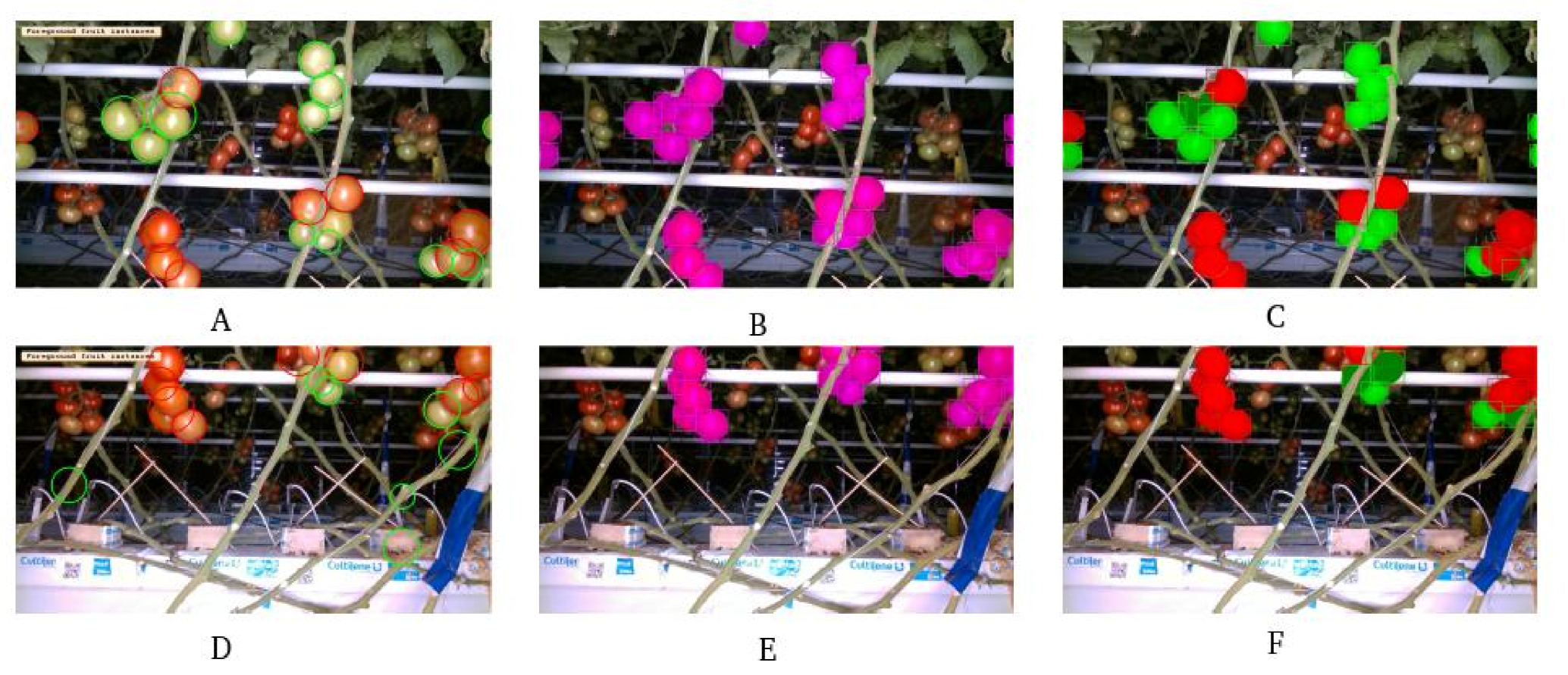
• Tomato detection by Mask-Region-based Convolutional Neural Networks (MaskRCNN)
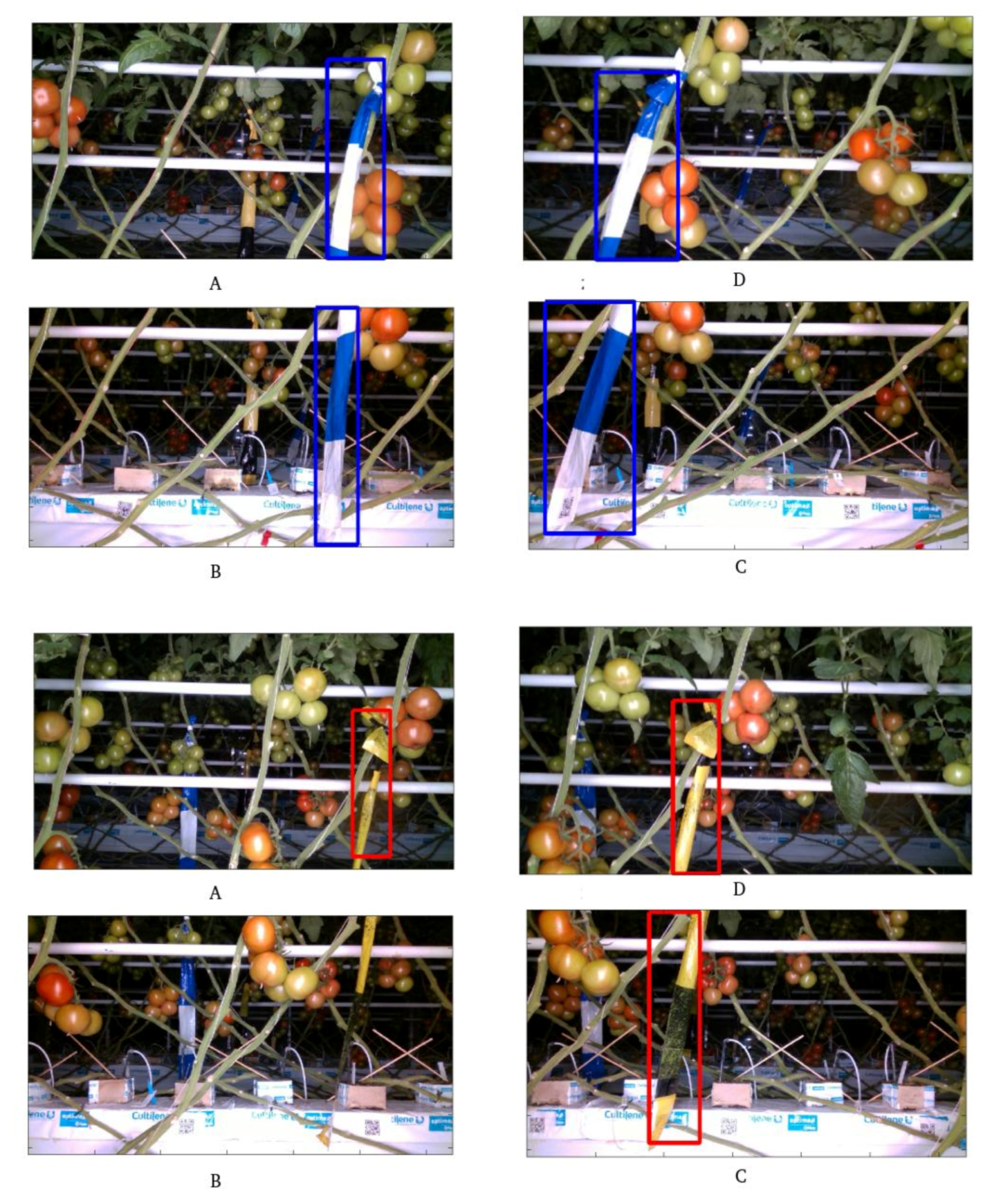
• Ribbon detection Faster Region-based Convolutional Neural Networks (FasterRCNN)
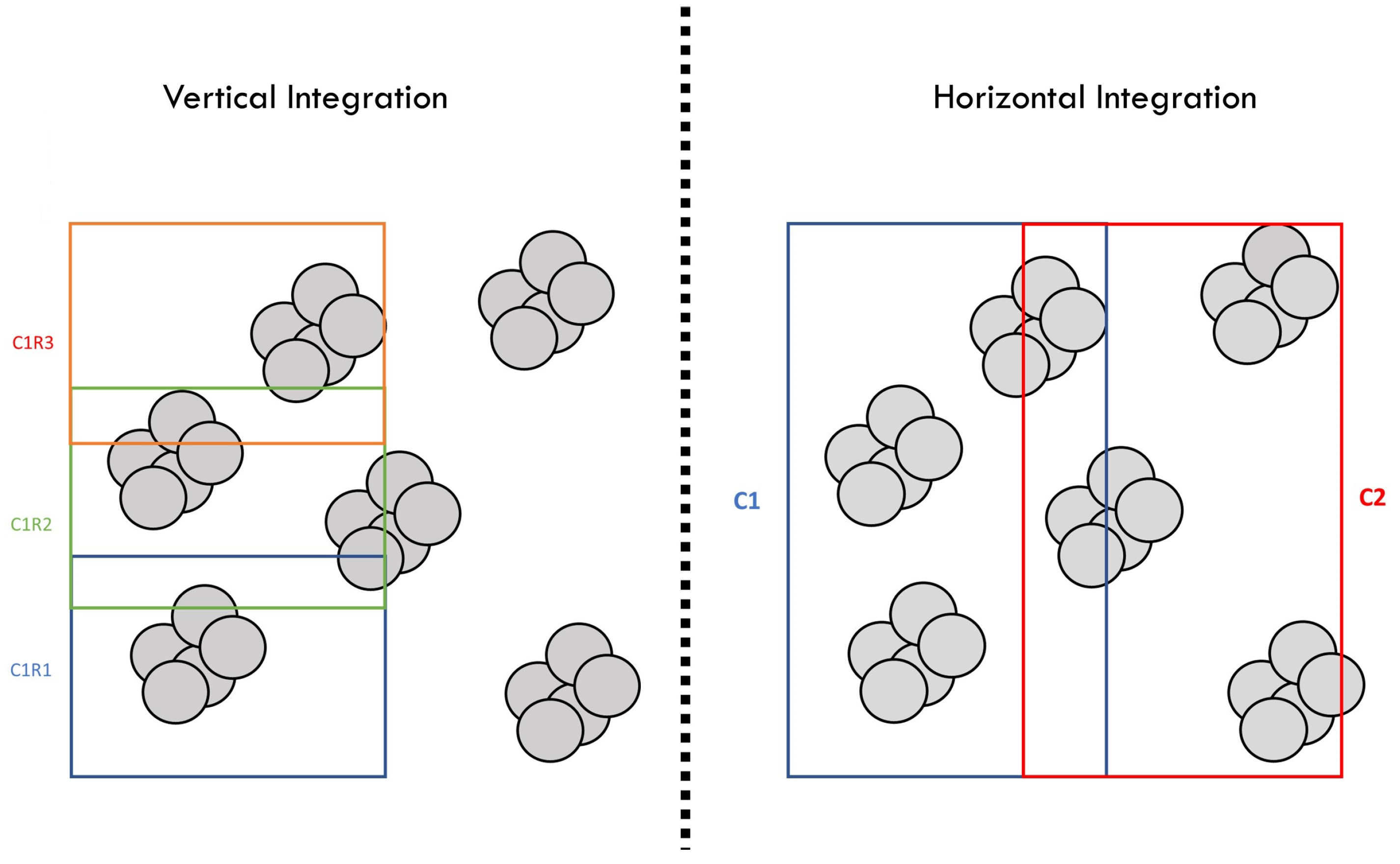
• Image registration (both vertically and horizontally, using a Discrete Fourier Transform (DFT)-based registration)
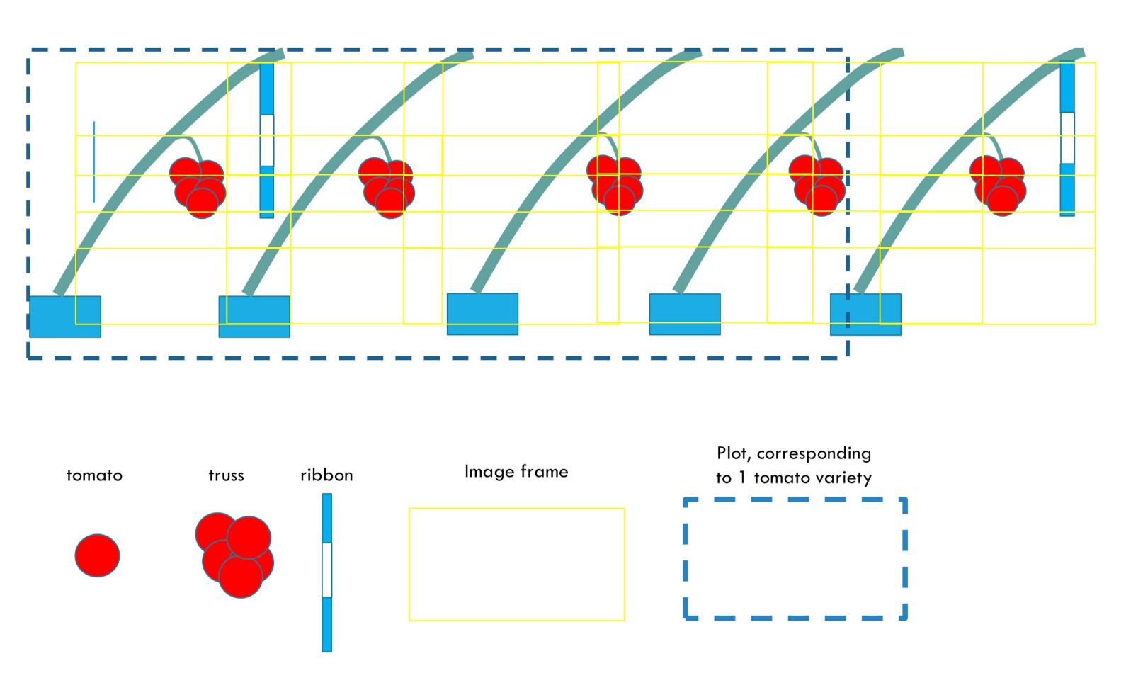
• Creation of a unified reference frame corresponding to a full row
• Position tomatoes and ribbons within this reference frame and assign tomatoes to plots

These steps are performed both for the pre- and for the post-harvest row images. We investigate the performance of this setup by comparing the ground-truth harvest yield (average weight per plot) with two predictors: the first based on only on the pre-harvest plot-level average tomato radius and the second based on a combination of an estimate of which tomatoes were harvested (by comparing pre- and post-harvest data) and the average tomato radius of the harvested tomato only. The first comparison is closest to a setup in which tomatoes are continuously monitored to predict harvest yield, as here only current pre-harvest data can be used, while the second comparison provides the closest comparison with the ground-truth. The second comparison involves two extra analysis steps:

• Truss detection (Connected-component analysis);
• Identification of harvested trusses by comparison between pre- and post-harvest data.

The Deep Learning algorithms (MaskRCNN, FasterRCNN) were run on a Linux Mint system with an NVIDIA Titan XP 12 GB GPU, while the rest of the processing pipeline was implemented as a set of MATLAB scripts and run on Intel i5 based laptops running either Windows 10 or Linux Mint. The following sections detail the processing steps outlined above.

2.3.1. Fruit Detection

For detecting fruits from individual images, we use Detectron MaskRCNN [48], a deep learning object detector, which we have previously used in [46]. This software was chosen as it can detect not only the bounding boxes of the fruits, but also the instance pixel masks. The model based on the 101 layer ResNext [49] backbone was trained on a set of manually annotated images taken in May and June 2019, before the data sets used for this study were acquired. The training set, which is available online (https://data.4tu.nl/articles/dataset/Rob2Pheno_Annotated_Tomato_Image_Dataset/13173422, accessed on 16 July 2021), is relatively small with 123 images, and contains images taken between two weeks and one month before the images analyzed in the present paper. In all cases, the images were taken at night and the LED flash illumination system was used to try and keep the illumination settings consistent.

This detection model is applied on all the images from each of the pre- and post-harvest data sets. For each detected tomato, the center coordinates and radius in pixels are estimated by fitting a circle to the tomato circumference. In the case of occluded tomatoes, only the longest circular portion of the object contour is used for this fitting. The resulting center coordinates and radii, in both pixels and millimeters, are saved in a CSV file by a MATLAB script, for the next parts of the processing pipeline.

2.3.2. Ribbon Detection

The plots of 4 plants of a single variety are separated by blue-white or yellow-black ribbons. Separation of these plots therefore requires ribbon detection. We use the FasterRCNN deep learning object detector [50] trained on 2 classes for each of the ribbon types. The training data for ribbon detection consisted of one entire row, which was annotated manually by drawing bounding boxes around the ribbons. After ribbon detection, the center coordinates of the detected ribbons are saved in a separate CSV file. As we have the sequence of plot varieties, we can match the tomatoes between a pair of ribbons to the corresponding plot.

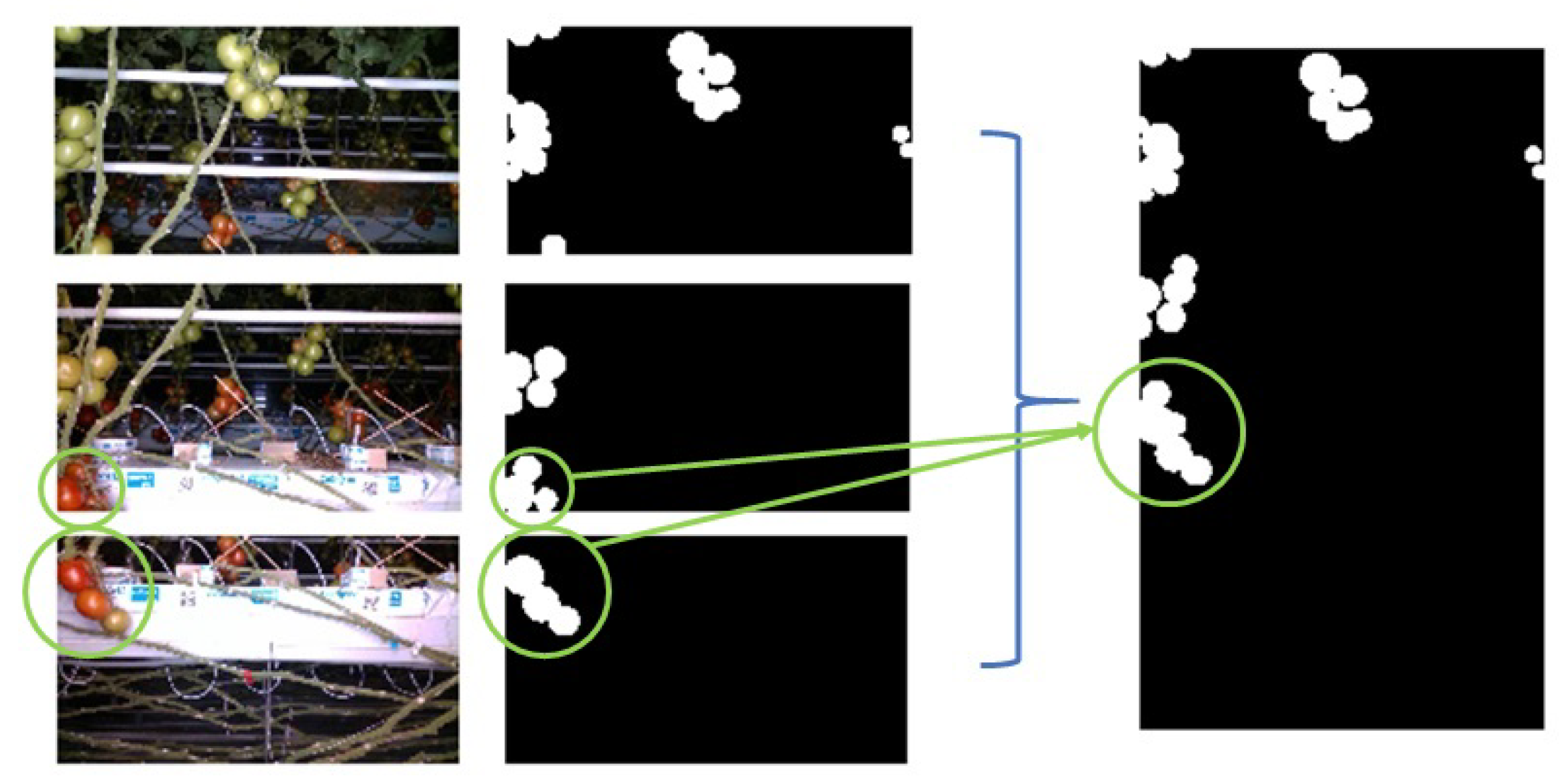
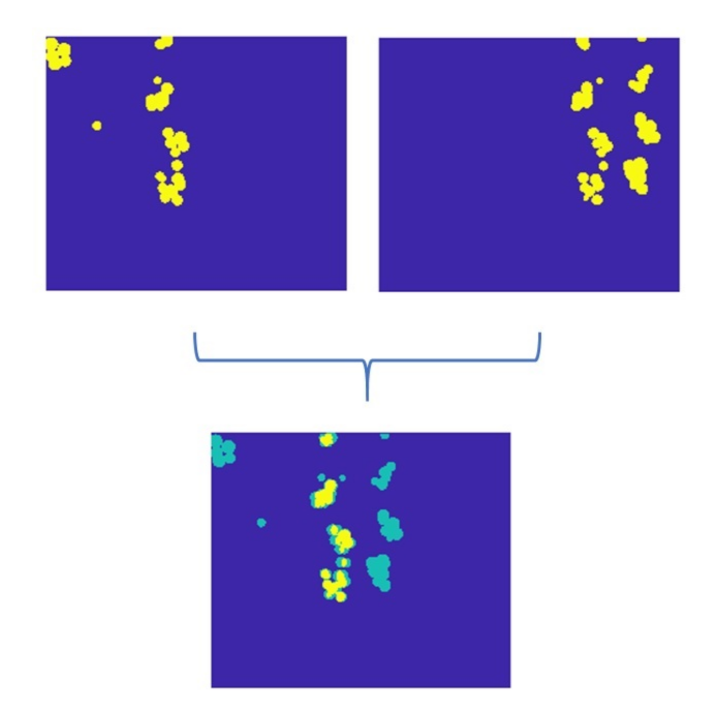
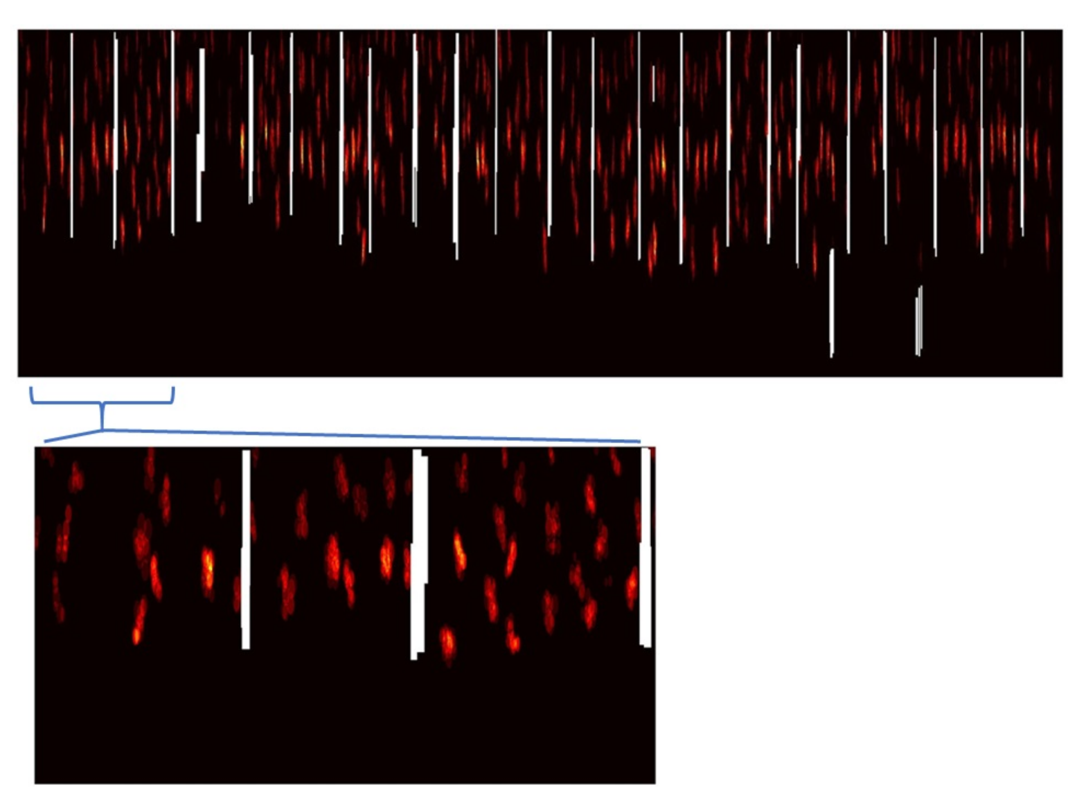
2.4. Image Registration

The acquired images display a large degree of overlap both horizontally and vertically. It is therefore necessary to create a scene for each row which contains all detected tomatoes and ribbons. The use of stitching algorithms based on feature detection and matching has proven difficult, as the objects of interest (tomatoes) are placed relatively close to the camera which, in combination with the background at greater distance, causes substantial parallax problems. We have therefore used a combination of depth-masking, tomato detection and an intensity-based registration algorithm as will be explained below. This resulted in the creation of a unified spatial reference frame in which all tomatoes and ribbons from a row are consistently positioned. The starting (x = 0, y = 0) coordinate corresponds to the lower left corner of the first image in the row.

Figure 4 illustrates the registration steps necessary to combine the images to form a unified spatial reference frame for the tomatoes and ribbons. As outlined in Section 2.2, each row is covered by a set of images that overlap both vertically and horizontally. The registration procedure starts by integrating images from the three different cameras (C1R1, C1R2, and C1R3 in Figure 4) vertically into column images (C1 and C2 in Figure 4). These column images are then again registered in the horizontal direction. The resulting transformations are then used to position the ribbon and tomato center coordinates into the unified reference frame.

We use a mixture of the original RGB images and the segmented tomato images as a basis for registration. This mixture is heavily biased towards the tomato segmentations, such that, if tomatoes are present, the segmented tomatoes will dominate the registration, but when few tomatoes are present (such as in some post-harvest images), the background provides sufficient extra information to perform successful registration. This has allowed the image registration to be based mainly on the image data that is most important (segmented tomatoes and ribbons).

We use a Discrete Fourier Transform (DFT)-based registration algorithm [51], which is an intensity-based registration algorithm that finds the optimal transformation of the moving image with respect to the target image, with the correlation between images as objective function. We further constrain this algorithm by only allowing translations (movements in the horizontal and vertical directions, no rotations or scaling) and by only allowing limited horizontal and vertical translations. These constraints were necessary, as the sparse nature of the available image data caused substantial mismatches when running performing DFT algorithm without optimization constraints.

As we expect the images from each vertical position on the robot to have a consistent position with respect to each other at each horizontal stopping position along the row, we only performed vertical registration on a limited subset of images and applied the median of the resulting vertical registration parameter sets on the full set of images. This creates the column images in Figure 4) for which we perform horizontal registration for each separate (column) image pair.

2.5. Truss Detection

We perform truss detection to identify the harvested trusses in a later stage. A truss in an tomato segmentation image is characterized by a large contiguous area of (partially) overlapping tomatoes. We have therefore performed a simple connected-components analysis using an 8-connected structuring element with a small minimum component size threshold to remove spurious trusses.

2.6. Detection of Harvested Trusses

So far, we have outlined the part of the image analysis pipeline that segments tomatoes and ribbons and places them in a unified reference frame for each row. We perform these steps separately for each row’s pre- and post-harvest acquisition. The following steps identify trusses in the pre-harvest row reference frame that are missing in the post-harvest row reference frame. We start by assuming that the position of the tomato trusses relative to the ribbons does not change between pre- and post-harvest acquisitions. This allows us to create an image of trusses for each plot pre- and post-harvest, with the starting position of the ribbon where the plot starts as the x = 0 coordinate. The overlap between pre- and post-harvest trusses then determines whether a pre-harvest truss has a corresponding post-harvest truss. The pre-harvest trusses that do not have a corresponding post-harvest truss are assumed to be harvested.

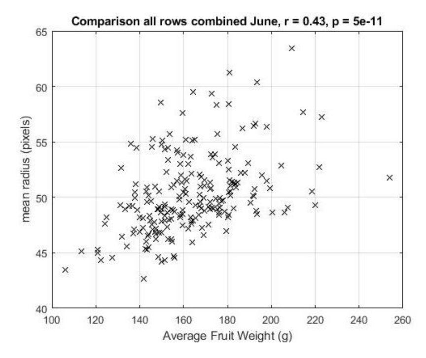
2.7. Comparison of Plot-Level Average Tomato Radius to Harvest Yield

The image analysis pipeline concludes by performing a statistical analysis of the average radius of tomatoes within harvested trusses (as detected by the algorithm) and its correspondence with the plot-level average tomato weight, as measured by the total weight of the tomatoes harvested per plot, divided by total number of tomatoes harvested per plot.

3. Results

3.1. Fruit Segmentation

An example of fruit detection using MaskRCNN is shown in Figure 5. In [46], we reported that the precision, recall, and F1 metrics were above $0.9$ for both the single fruit class and two ripeness classes. Figure 5 also shows an example of segmentation based on a more classical computer vision algorithm using color space transforms and shape fitting. These results are shown in Figure 5A,D as red or green contours indicating the detected fruits. MaskRCNN clearly outperforms the alternative algorithm by missing fewer fruits and detecting fewer false positives. For more examples, please refer to the work in [46] and the associated supplementary material.

3.2. Ribbon Segmentation

Figure 6 shows the detection of the plot separator ribbons using FasterRCNN. It is interesting to note that, even when a ribbon gets missed in one image due to its orientation with respect to the camera, it is detected in neighboring images. The ribbon detection still required manual correction to remove large ribbons from the row behind the current row—the depth images did not always provide enough information to distinguish between ribbons in the foreground and ribbons in the background.

3.3. Image Registration

As outlined in Section 2.4, the registration algorithm starts by vertically integrating the images of the three cameras at each position in the row into column images. Figure 7 shows an example of the results of this vertical integration. This shows good integration, for instance, when comparing the circled truss of the middle left image and the corresponding circled truss in the lower left image and how they are integrated in the column image.

Figure 8 shows an example of the horizontal registration of the column images. Again, good overlap can be observed between corresponding trusses in adjacent column images. Note that both vertical and horizontal registration results in double-counting of tomatoes because all originally detected tomatoes are integrated into the final row reference frame.

Figure 9 shows the results of combining the horizontal and vertical registration over the full row as a heat map showing the overlap of the segmented tomatoes from the individual images when transformed to the row-based reference frame. This procedure results in clearly separated trusses, which can then be used for further processing. This result might suggest that segmentation could simply be performed on the integrated RGB image of the full row. However, a careful inspection of the trusses in such images shows that there are too many discontinuities for the segmentation algorithm to perform well.

3.4. Overall Performance

For an assessment of the overall performance, we concentrate on image estimates of yield, expressed as average fruit radii per plot. Figure 10 shows a scatter plot of the predicted average fruit radius per plot, and the average fruit weight as measured after harvesting the fruits. Here, we have only analyzed the pre-harvest images and therefore have included all tomatoes into the analysis, regardless of whether they are harvested or not. This plot shows a reasonable correspondence between predicted fruit radius and measured fruit weight ($r=0.43,p=5e^{-11}$), albeit with an increased variance at higher fruits weights. An analysis including pre- and post-harvest images, including truss detection and identification of harvested trusses yielded very similar results.

A breakdown of the relationship between plot-level average tomato radius and measured weight per row (not shown) indicates that performance can vary substantially across rows. We should note, however, that the limited number of data points per row precludes any firm conclusions.

4. Discussion

This project and related work have demonstrated that image acquisition is effective: the combination of a relatively low-tech robot, which uses the already present heating pipes of the greenhouse and low-cost commercially available cameras proved, after initial setup issues, to be reliable and to deliver images of sufficient quality for the segmentation algorithm. The night-time acquisition schedule (in combination with the LED-based illumination system) is advantageous because it ensures constant illumination conditions, which in turn ensures constant performance of the segmentation algorithm. In addition, it does not interfere with day-to-day operations in the greenhouse. Segmentation, as described in [47], showed high performance, which is especially remarkable since the training data set in this paper is relatively modest. Adaptation to a new environment should therefore be relatively painless.

Image registration and the construction of a row-based reference system for the detected tomatoes was more complicated. This step is necessary when it is not possible to image the whole plant or unit of harvest as was done in [31] in which entire apple trees were covered in one image. Both vertical and horizontal integration was necessary: vertical to integrate the views of the three different cameras and horizontal integration to integrate the views from different stops of the robot along the row. Both types of integration were performed sequentially (vertical first, then horizontal) by a heavily modified version of a fast DFT-based registration algorithm [51]. The registration approach relies on both segmentation results and the RGB images themselves—registration based mainly on the segmentation results makes the registration much less complex and reduces the parallax problem considerably, while the addition of the RGB background was necessary to register images with only few detected tomatoes, which is the case in many post-harvest images. Apart from this process of feature adaptation for the registration algorithm, we also heavily constrained the DFT-based registration optimization procedure to only allow solutions in a narrow range of horizontal and vertical shifts.

Although the integration of images into a coherent row-based reference frame was successful, this does not completely solve the problem of placing detected fruits into this reference frame: many fruits will be present in multiple images, which leads to double counting. Extensive experimentation with rule-based double-counting solutions, based on the fact that tomatoes that are present in different images should show high overlap when creating the row-based representation, did not improve the total results.

We use the fruit radius as predicted by Deep Learning to compare with the fruit weight as measured during harvest. The fruits were already selected to fall within a limited depth range to focus only on fruits from the row immediately in front of the camera. Hence, depth information is used implicitly in determining fruit radii. Because of the limited depth resolution of the cameras no further improvement in the precision of the radius estimates is to be expected-prediction accuracy is dominated by other aspects, as detailed in the following paragraphs.

Another difficulty is occlusion. Tomatoes are not fully visible in all images: tomatoes within trusses already show heavy overlap. Other occlusions are caused by objects such as pipes, tomato stems and the ribbons used to delineate plots. There will always be fruits for which accurate measurements are impossible because of occlusion. This, however, is one of the reasons behind high-throughput phenotyping: if a greenhouse can be completely covered every night, or every other night, then errors will cancel out and a consistent trend will emerge from the data.

The aforementioned occlusion problem caused by the ribbons introduces another problem when assigning tomatoes to plots: for tomatoes that are occluded by ribbons it is unclear whether to assign those tomatoes to the plot anterior or posterior to the ribbon. Moreover, in some cases tomato trusses from a tomato plant anterior to a ribbon are posterior to the same ribbon, because of the diagonal alignment of the tomato plants, leading to further erroneous assignments. The introduction of ribbons to delineate plots can therefore be improved upon, for instance by marking each truss or even tomato with a label indicating its corresponding plot. However, these labels would not be visible in all images and would moreover introduce another labor-intensive step into the phenotyping process, which is undesirable.

Ultimately, one would want to go beyond plot-based comparisons and be able to segment and identify tomatoes and their corresponding plants. This would alleviate the above mentioned assignment problem as well, as each plant could easily be coded by a label at the pot, and trusses and tomatoes could be identified by their distance from the pot along the stem. However, stem tracking in typical greenhouse setups is complicated because stems of the same row more often than not overlap and/or cross.

In conclusion, our work shows that, although significant progress has been made on the individual components of an automatic phenotyping system, the setup in which such as system is deployed, in our case a breeding greenhouse, will often present significant challenges. Meeting these challenges goes beyond improvements of the individual components and requires careful consideration of the experimental setup. Further improvements in camera systems (e.g., better depth information, or wider fields of view), and decreasing costs for hardware (making it possible to employ, say, eight cameras instead of four so that parallax problems are minimized and image registration becomes much easier because of increased overlap) will undoubtedly help.

References

1. Furbank, R.T.; Tester, M. Phenomics—Technologies to relieve the phenotyping bottleneck. Trends Plant Sci. 2011, 16, 635–644. [Google Scholar] [CrossRef]
2. Li, L.; Zhang, Q.; Huang, D. A review of imaging techniques for plant phenotyping. Sensors 2014, 14, 20078–20111. [Google Scholar] [CrossRef]
3. Minervini, M.; Scharr, H.; Tsaftaris, S.A. Image Analysis: The New Bottleneck in Plant Phenotyping [Applications Corner]. IEEE Signal Process. Mag. 2015, 32, 126–131. [Google Scholar] [CrossRef] [Green Version]
4. LeCun, Y.; Bengio, Y.; Hinton, G. Deep learning. Nature 2015, 521, 436. [Google Scholar] [CrossRef] [PubMed]
5. Kamilaris, A.; Prenafeta-Boldú, F.X. Deep learning in agriculture: A survey. Comput. Electron. Agric. 2018, 147, 70–90. [Google Scholar] [CrossRef] [Green Version]
6. Das Choudhury, S.; Samal, A.; Awada, T. Leveraging image analysis for high-throughput plant phenotyping. Front. Plant Sci. 2019, 10, 508. [Google Scholar] [CrossRef] [PubMed]
7. Abade, A.S.; Ferreira, P.A.; Vidal, F.d.B. Plant Diseases recognition on images using Convolutional Neural Networks: A Systematic Review. arXiv 2020, arXiv:2009.04365. [Google Scholar]
8. Burud, I.; Lange, G.; Lillemo, M.; Bleken, E.; Grimstad, L.; From, P.J. Exploring robots and UAVs as phenotyping tools in plant breeding. IFAC-PapersOnLine 2017, 50, 11479–11484. [Google Scholar] [CrossRef]
9. Johansen, K.; Morton, M.J.; Malbeteau, Y.; Aragon, B.J.L.; AlMashharawi, S.; Ziliani, M.; Angel, Y.; Fiene, G.; Negrao, S.; Mousa, M.A.; et al. Predicting Biomass and Yield in a Tomato Phenotyping Experiment using UAV Imagery and Machine Learning. Front. Artif. Intell. 2020, 3, 28. [Google Scholar] [CrossRef]
10. Granier, C.; Aguirrezabal, L.; Chenu, K.; Cookson, S.J.; Dauzat, M.; Hamard, P.; Thioux, J.J.; Rolland, G.; Bouchier-Combaud, S.; Lebaudy, A.; et al. PHENOPSIS, an automated platform for reproducible phenotyping of plant responses to soil water deficit in Arabidopsis thaliana permitted the identification of an accession with low sensitivity to soil water deficit. New Phytol. 2006, 169, 623–635. [Google Scholar] [CrossRef]
11. Walter, A.; Scharr, H.; Gilmer, F.; Zierer, R.; Nagel, K.A.; Ernst, M.; Wiese, A.; Virnich, O.; Christ, M.M.; Uhlig, B.; et al. Dynamics of seedling growth acclimation towards altered light conditions can be quantified via GROWSCREEN: A setup and procedure designed for rapid optical phenotyping of different plant species. New Phytol. 2007, 174, 447–455. [Google Scholar] [CrossRef] [PubMed]
12. Reuzeau, C. TraitMill (TM): A high throughput functional genomics platform for the phenotypic analysis of cereals. In In Vitro Cellular & Developmental Biology-Animal; Springer: New York, NY, USA, 2007; Volume 43, p. S4. [Google Scholar]
13. Tang, Y.C.; Wang, C.; Luo, L.; Zou, X. Recognition and localization methods for vision-based fruit picking robots: A review. Front. Plant Sci. 2020, 11, 510. [Google Scholar] [CrossRef] [PubMed]
14. Kootstra, G.; Wang, X.; Blok, P.M.; Hemming, J.; van Henten, E. Selective Harvesting Robotics: Current Research, Trends, and Future Directions. Curr. Robot. Rep. 2021, 1–10. [Google Scholar] [CrossRef]
15. Hemming, J.; Bac, C.W.; Van Tuijl, B.; Barth, R.; Bontsema, J.; Pekkeriet, E. A robot for harvesting sweet-pepper in greenhouses. In Proceedings of the International Conference of Agricultural Engineering, Lausanne, Switzerland, 6–10 October 2014. [Google Scholar]
16. Bac, C.W.; Hemming, J.; van Tuijl, B.; Barth, R.; Wais, E.; van Henten, E.J. Performance Evaluation of a Harvesting Robot for Sweet Pepper. J. Field Robot. 2017, 34, 1123–1139. [Google Scholar] [CrossRef]
17. Ringdahl, O.; Kurtser, P.; Barth, R.; Edan, Y. Operational Flow of an Autonomous Sweetpepper Harvesting Robot. BO-25.06-002-003-PPO/PRI, EU-2015-03, 1409-035 EU. 2016. Available online: http://edepot.wur.nl/401245 (accessed on 6 August 2021).
18. Barth, R.; IJsselmuiden, J.; Hemming, J.; Van Henten, E.J. Optimising Realism of Synthetic Agricultural Images Using Cycle Generative Adversarial Networks; Wageningen University & Research: Wageningen, The Netherlands, 2017. [Google Scholar]
19. Mao, S.; Li, Y.; Ma, Y.; Zhang, B.; Zhou, J.; Wang, K. Automatic cucumber recognition algorithm for harvesting robots in the natural environment using deep learning and multi-feature fusion. Comput. Electron. Agric. 2020, 170, 105254. [Google Scholar] [CrossRef]
20. Oberti, R.; Marchi, M.; Tirelli, P.; Calcante, A.; Iriti, M.; Tona, E.; Hočevar, M.; Baur, J.; Pfaff, J.; Schütz, C.; et al. Selective spraying of grapevines for disease control using a modular agricultural robot. Biosyst. Eng. 2016, 146, 203–215. [Google Scholar] [CrossRef]
21. Paulin, S.; Botterill, T.; Lin, J.; Chen, X.; Green, R. A comparison of sampling-based path planners for a grape vine pruning robot arm. In Proceedings of the 2015 6th International Conference on Automation, Robotics and Applications (ICARA), Queenstown, New Zealand, 17–19 February 2015; IEEE: New York, NY, USA, 2015; pp. 98–103. [Google Scholar]
22. Kaljaca, D.; Vroegindeweij, B.; Henten, E.J.V. Coverage trajectory planning for a bush trimming robot arm. J. Field Robot. 2019, 1–26. [Google Scholar] [CrossRef] [Green Version]
23. Cuevas-Velasquez, H.; Gallego, A.J.; Tylecek, R.; Hemming, J.; van Tuijl, B.; Mencarelli, A.; Fisher, R.B. Real-time Stereo Visual Servoing for Rose Pruning with Robotic Arm. In Proceedings of the 2020 International Conference on Robotics and Automation, Paris, France, 31 May–31 August 2020. [Google Scholar]
24. Ruckelshausen, A.; Biber, P.; Dorna, M.; Gremmes, H.; Klose, R.; Linz, A.; Rahe, F.; Resch, R.; Thiel, M.; Trautz, D.; et al. BoniRob–an autonomous field robot platform for individual plant phenotyping. Precis. Agric. 2009, 9, 1. [Google Scholar]
25. van der Heijden, G.; Song, Y.; Horgan, G.; Polder, G.; Dieleman, A.; Bink, M.; Palloix, A.; van Eeuwijk, F.; Glasbey, C. SPICY: Towards automated phenotyping of large pepper plants in the greenhouse. Funct. Plant Biol. 2012, 39, 870–877. [Google Scholar] [CrossRef]
26. Zhou, J.; Chen, H.; Zhou, J.; Fu, X.; Ye, H.; Nguyen, H.T. Development of an automated phenotyping platform for quantifying soybean dynamic responses to salinity stress in greenhouse environment. Comput. Electron. Agric. 2018, 151, 319–330. [Google Scholar] [CrossRef]
27. Shah, D.; Tang, L.; Gai, J.; Putta-Venkata, R. Development of a Mobile Robotic Phenotyping System for Growth Chamber-based Studies of Genotype x Environment Interactions. IFAC-PapersOnLine 2016, 49, 248–253. [Google Scholar] [CrossRef]
28. Zhang, J.; Gong, L.; Liu, C.; Huang, Y.; Zhang, D.; Yuan, Z. Field Phenotyping Robot Design and Validation for the Crop Breeding. IFAC-PapersOnLine 2016, 49, 281–286. [Google Scholar] [CrossRef]
29. Virlet, N.; Sabermanesh, K.; Sadeghi-Tehran, P.; Hawkesford, M.J. Field Scanalyzer: An automated robotic field phenotyping platform for detailed crop monitoring. Funct. Plant Biol. 2016, 44, 143–153. [Google Scholar] [CrossRef] [Green Version]
30. Boogaard, F.P.; Rongen, K.S.; Kootstra, G.W. Robust node detection and tracking in fruit-vegetable crops using deep learning and multi-view imaging. Biosyst. Eng. 2020, 192, 117–132. [Google Scholar] [CrossRef]
31. Bargoti, S.; Underwood, J.P. Image segmentation for fruit detection and yield estimation in apple orchards. J. Field Robot. 2017, 34, 1039–1060. [Google Scholar] [CrossRef] [Green Version]
32. Liu, X.; Chen, S.W.; Liu, C.; Shivakumar, S.S.; Das, J.; Taylor, C.J.; Underwood, J.; Kumar, V. Monocular camera based fruit counting and mapping with semantic data association. IEEE Robot. Autom. Lett. 2019, 4, 2296–2303. [Google Scholar] [CrossRef] [Green Version]
33. Huang, J.; Rathod, V.; Sun, C.; Zhu, M.; Korattikara, A.; Fathi, A.; Fischer, I.; Wojna, Z.; Song, Y.; Guadarrama, S.; et al. Speed/accuracy trade-offs for modern convolutional object detectors. In Proceedings of the IEEE Conference on Computer Vision and Pattern Recognition, Honolulu, HI, USA, 21–26 July 2017; pp. 7310–7311. [Google Scholar]
34. Mu, Y.; Chen, T.S.; Ninomiya, S.; Guo, W. Intact Detection of Highly Occluded Immature Tomatoes on Plants Using Deep Learning Techniques. Sensors 2020, 20, 2984. [Google Scholar] [CrossRef] [PubMed]
35. Koller, M.; Upadhyaya, S. Prediction of processing tomato yield using a crop growth model and remotely sensed aerial images. Trans. ASAE 2005, 48, 2335–2341. [Google Scholar] [CrossRef]
36. Ashapure, A.; Oh, S.; Marconi, T.G.; Chang, A.; Jung, J.; Landivar, J.; Enciso, J. Unmanned aerial system based tomato yield estimation using machine learning. In Autonomous Air and Ground Sensing Systems for Agricultural Optimization and Phenotyping IV; International Society for Optics and Photonics: Bellingham, WA, USA, 2019; Volume 11008, p. 110080O. [Google Scholar]
37. Darrigues, A.; Hall, J.; van der Knaap, E.; Francis, D.M.; Dujmovic, N.; Gray, S. Tomato analyzer-color test: A new tool for efficient digital phenotyping. J. Am. Soc. Hortic. Sci. 2008, 133, 579–586. [Google Scholar] [CrossRef] [Green Version]
38. Stein, M.; Bargoti, S.; Underwood, J. Image Based Mango Fruit Detection, Localisation and Yield Estimation Using Multiple View Geometry. Sensors 2016, 16, 1915. [Google Scholar] [CrossRef] [PubMed]
39. Schonberger, J.L.; Frahm, J.M. Structure-from-motion revisited. In Proceedings of the IEEE Conference on Computer Vision and Pattern Recognition, Las Vegas, NV, USA, 27–30 June 2016; pp. 4104–4113. [Google Scholar]
40. Fujinaga, T.; Yasukawa, S.; Li, B.; Ishii, K. Image mosaicing using multi-modal images for generation of tomato growth state map. J. Robot. Mechatron. 2018, 30, 187–197. [Google Scholar] [CrossRef]
41. Gan, H.; Lee, W.S.; Alchanatis, V. A photogrammetry-based image registration method for multi-camera systems–With applications in images of a tree crop. Biosyst. Eng. 2018, 174, 89–106. [Google Scholar] [CrossRef]
42. Liu, X.; Chen, S.W.; Aditya, S.; Sivakumar, N.; Dcunha, S.; Qu, C.; Taylor, C.J.; Das, J.; Kumar, V. Robust fruit counting: Combining deep learning, tracking, and structure from motion. In Proceedings of the 2018 IEEE/RSJ International Conference on Intelligent Robots and Systems (IROS), Madrid, Spain, 1–5 October 2018; IEEE: New York, NY, USA, 2018; pp. 1045–1052. [Google Scholar]
43. Badrinarayanan, V.; Kendall, A.; Cipolla, R. SegNet: A Deep Convolutional Encoder-Decoder Architecture for Image Segmentation. IEEE Trans. Pattern Anal. Mach. Intell. 2017, 39, 2481–2495. [Google Scholar] [CrossRef] [PubMed]
44. Matsuzaki, S.; Masuzawa, H.; Miura, J.; Oishi, S. 3D Semantic Mapping in Greenhouses for Agricultural Mobile Robots with Robust Object Recognition Using Robots’ Trajectory. In Proceedings of the 2018 IEEE International Conference on Systems, Man, and Cybernetics (SMC), Miyazaki, Japan, 7–10 October 2018; pp. 357–362. [Google Scholar]
45. Gené-Mola, J.; Sanz-Cortiella, R.; Rosell-Polo, J.R.; Morros, J.R.; Ruiz-Hidalgo, J.; Vilaplana, V.; Gregorio, E. Fruit detection and 3D location using instance segmentation neural networks and structure-from-motion photogrammetry. Comput. Electron. Agric. 2020, 169, 105165. [Google Scholar] [CrossRef]
46. Afonso, M.; Fonteijn, H.; Fiorentin, F.S.; Lensink, D.; Mooij, M.; Faber, N.; Polder, G.; Wehrens, R. Tomato Fruit Detection and Counting in Greenhouses Using Deep Learning. Front. Plant Sci. 2020, 11, 1759. [Google Scholar] [CrossRef]
47. Afonso, M.; Mencarelli, A.; Polder, G.; Wehrens, R.; Lensink, D.; Faber, N. Detection of tomato flowers from greenhouse images using colorspace transformations. In Proceedings of the EPIA Conference on Artificial Intelligence, Vila Real, Portugal, 3–6 September 2019; pp. 146–155. [Google Scholar]
48. He, K.; Gkioxari, G.; Dollár, P.; Girshick, R. Mask r-cnn. In Proceedings of the 2017 IEEE International Conference on Computer Vision (ICCV), Venice, Italy, 22–29 October 2017; IEEE: New York, NY, USA, 2017; pp. 2980–2988. [Google Scholar]
49. Xie, S.; Girshick, R.; Dollár, P.; Tu, Z.; He, K. Aggregated residual transformations for deep neural networks. In Proceedings of the 2017 IEEE Conference on Computer Vision and Pattern Recognition (CVPR), Honolulu, HI, USA, 21–26 July 2017; IEEE: New York, NY, USA, 2017; pp. 5987–5995. [Google Scholar]
50. Girshick, R. Fast R-CNN. In Proceedings of the 2015 IEEE International Conference on Computer Vision (ICCV), Santiago, Chile, 7–13 December 2015; pp. 1440–1448. [Google Scholar] [CrossRef]
51. Guizar-Sicairos, M.; Thurman, S.T.; Fienup, J.R. Efficient subpixel image registration algorithms. Opt. Lett. 2008, 33, 156–158. [Google Scholar] [CrossRef] [PubMed] [Green Version]
Figure 1. The Phenobot in its starting position in the greenhouse.
Agronomy 11 01599 g001
Figure 2. An example of a sequence of images over one plot. The images taken by the four cameras are stacked vertically according to camera position. Each plot consists of four plants of the same variety, delimited by the blue and white ribbons.
Agronomy 11 01599 g002
Figure 3. A stylized representation of the elements necessary to process image-level data to create plot-level yield predictions. The blue-white ribbon indicates the start of a plot containing four plants. The image boundaries for each camera are shown in yellow.
Agronomy 11 01599 g003
Figure 4. Illustration of the vertical and horizontal registration necessary to integrate across rows.
Agronomy 11 01599 g004
Figure 5. Example of detection of fruits using: (A,D) classical shape and colorspace segmentation, (B,E) MaskRCNN with one fruit class, (C,F) MaskRCNN with two ripeness classes.
Agronomy 11 01599 g005
Figure 6. Plot demarcation: examples of detection of 2 ribbons in groups of neighboring images. We see that if a ribbon gets missed in one image, it can get detected in neighboring ones.
Agronomy 11 01599 g006
Figure 7. Example of vertical registration. The three images in the left column are original RGB images of the three cameras at one position in the row. The middle column shows the detected fruits at each camera position. The right column shows the integrated column image, with good integration of the overlapping trusses. Note that the dimensions of column image are different as they incorporate the overlap between the images, which decreases the vertical size with respect to the sum of the vertical size of the 3 camera images.
Agronomy 11 01599 g007
Figure 8. Example of horizontal registration. The upper panel shows detected trusses from two adjacent column images. The lower panel shows the result of horizontal overlap, with nonoverlapping tomatoes shown in green and overlapping tomatoes shown in yellow. Again, good overlap can be observed where the column images overlap.
Agronomy 11 01599 g008
Figure 9. Example of final registration result. The upper panel shows all detected tomatoes from a full row with detected ribbons in white for reference. The color scale indicates the overlap of the detected fruits from the original images after integration into the row reference frame. The lower panel shows a zoomed in image from the row in the upper panel, covering 3 plots.
Agronomy 11 01599 g009
Figure 10. Scatter plot of predicted average fruit radius in pixels versus the average harvested fruit weight, over all rows.
Agronomy 11 01599 g010
Publisher’s Note: MDPI stays neutral with regard to jurisdictional claims in published maps and institutional affiliations.