This section describes the experiments performed to test the proposed approach. Firstly, the metrics used to evaluate the system are presented. Then, an evaluation is performed of the entire approach. Finally, an overall discussion of the obtained results is carried out.
4.1. Methodology
The evaluation performed used state-of-the-art metrics to evaluate the DL models deployed. In this work, seven different metrics were used: precision, recall, F1 score, precision × recall curve, AP, medium AP (mAP), and inference time. To calculate these metrics, the following set of concepts was used:
Interception over Union (IoU): a measure based on the Jaccard index that calculates the overlap between two bounding boxes using the ground truth and the predicted bounding boxes;
True Positive (TP): a valid detection, i.e., IoU ≥ threshold;
False Positive (FP): an invalid detection, i.e., IoU < threshold;
False Negative (FN): a ground truth bounding box not detected.
Given all of the above, the metrics were calculated as follows:
Precision: defined as the ability of a given model to detect only relevant objects, precision is calculated as the percentage of TP and is given by:
Recall: defined as the ability of a given model to find all the ground truth bounding boxes, recall is calculated as the percentage of TP detected divided by all the ground truths and is given by:
F1 score: defined as the harmonic mean between precision and recall, F1 score is given by:
Precision × recall curve: a curve plotted for each object class that shows the tradeoff between precision and recall;
AP: calculated as the area under the precision × recall curve. A high area represents both high precision and recall;
mAP: calculated as the mean AP for all the object classes;
Inference time: defined in this work as the amount of time that a model takes to process a tile or an image, on average.
In this work, the previously described metrics were used to evaluate both SSD MobileNet-V1 and SSD Inception-V2. In addition, the models were characterized by changing two parameters: the detection confidence and the IoU thresholds. Some visual results were also present to demonstrate the system robustness to occluded objects and variations in illumination conditions. To perform a fair evaluation of the DL models, the input dataset was divided into three groups: training, test, and evaluation. The larger one, the training set, was used to train the DL models. The test set was used to perform the evaluation of the models during the training by Tensorflow. The evaluation set was exclusively used to test the models by computing the metrics described above.
4.2. Evaluation
This work used quantized models to detect grape bunches at different growth stages. To evaluate these models, they were characterized by changing the confidence threshold and the IoU parameter.
Table 4 shows the detection performance of SSD MobileNet-V1 and SSD Inception-V2 for three values of the confidence: 30%, 50%, and 70%.
This table shows the effect of varying the confidence threshold. In particular, it is visible that when the confidence score increased, the precision also increased. This was due to the elimination of low-confidence detections. Thus, if we considered only the high-confidence detections, the model would be more suitable to detect only relevant objects, which would lead to an increase of the precision. On the contrary, when the confidence threshold increased, the number of TP decreased, which led to a decrease of the recall. Comparing both models, one can see that SSD Inception-V2 presented a higher precision than SSD MobileNet-V1 for all confidence scores, but a lower recall. This led to the conclusion that Inception presented a high rate of TP from all the detections, but a low rate of TP considering the ground truths. Overall, SSD MobileNet-V1 outperformed the Inception model, presenting a higher F1 score, AP, and mAP. This model achieved, as the best result, a mAP of 44.93% for a confidence score of 30%.
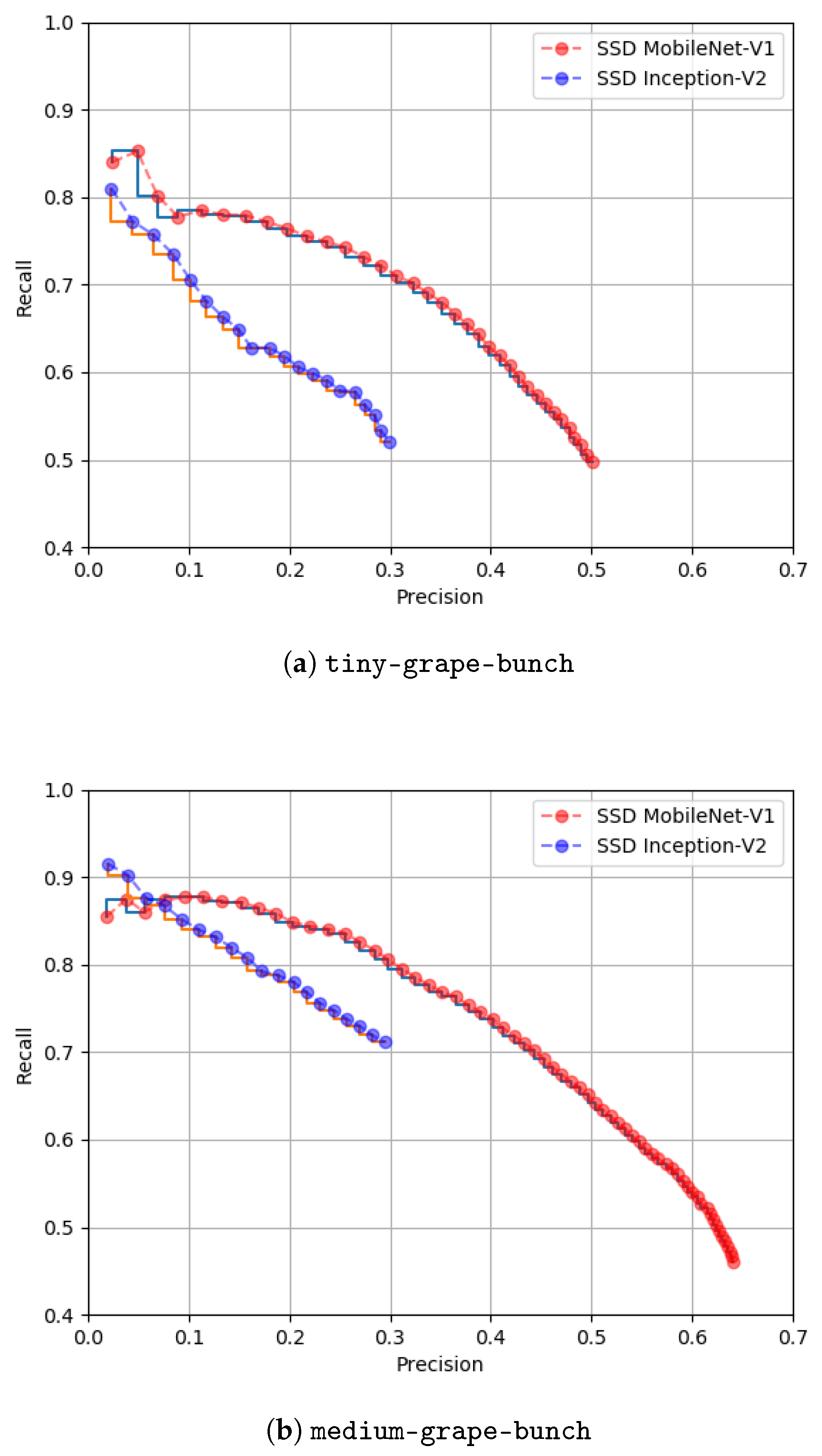
Figure 8 shows the precision × recall curves for both models considering the two classes and a confidence score of 50%.
Once again, this figure shows that SSD MobileNet-V1 outperformed the Inception model. Comparing the models performance detecting objects of both classes, we verified that detecting grape bunches at an early stage (
tiny-grape-bunch) was more challenging than at an intermediate growth stage (
medium-grape-bunch). The first class represented smaller grape bunches, with a color and texture more similar to the surrounding foliage, which complicated their detection. SSD MobileNet-V1 presented a AP of 40.38% detecting grape bunches at an early growth stage and 49.48% at an intermediate growth stage. Finally,
Figure 9 shows the impact of the confidence score on the detections for a single image.
One can verify that this parameter can be used to eliminate FPs that usually present low-confidence scores.
Table 5 presents the detection performance considering a variation of the IoU evaluation parameter.
This characterization was performed since different values for the overlap between detections and ground truths can give more information about the models’ performance. For example, lower IoU values would consider detections that, besides not corresponding exactly to the location of the ground truths, represent annotated objects that were actually detected. To evaluate this, three values for the IoU parameter were considered: 20%, 40%, and 60%. Once again, one can verify that the SSD Inception-V2 model presented a higher precision. For an IoU value of 20%, this model had a precision of 92.57% detecting grape bunches at an intermediate growth stage. This is a satisfactory result since it means that 92.57% of the detections were TPs. On the other side, SSD MobileNet-V1 presented high recall levels. For an IoU of 20%, it achieved a recall of 87.01% for the class medium-grape-bunch. For higher IoU values, the performance of both models decreased. This was expected since, for example, for an IoU of 60%, the detections that did not overlap more than 60% with the ground truths were considered as FPs, which led to a decrease in performance. Overall, the best result was achieved by SSD MobileNet-V1, which performed with a mAP of 66.96% for an IoU of 20%.
As referenced before, the models were deployed in a low-cost and low-power embedded device, a TPU. It was intended that these models run in a time-effective manner to be integrated in more complex systems such as harvesting and spraying procedures. Thus, evaluating the runtime performance of both models was important in the context of this work.
Table 6 shows the inference time results for both models.
In this table, the performances per tile and per image are both described. The inference time per tile was also considered in this evaluation since it represents the time that each model would take to process an entire image if the input images were not split. The inference times were measured for each evaluation image, and the final value considered was the average for all images. The results showed that the SSD MobileNet-V1 was more than four-times faster than the Inception model. This was due to the simpler architecture of MobileNets in relation to Inception, and the higher compatibility of MobileNet compared with Inception. This model can process a single tile in 6.29 ms and an entire split image in 93.12 ms. This proved both the high performance of the model, but also that the TPU hardware device used was capable of deploying models in a very efficient way, even considering low-power costs.
This approach was intended to be robust to different light conditions since the robot would operate at different times of the day and stages of the year. Because of this reason, the built dataset considered several light conditions, and the models were trained to be robust to them. Furthermore, the dataset considered occluded grape bunches so that the models could also detect not fully visible grape bunches. To demonstrate these challenging conditions present in the proposed dataset,
Figure 10 and
Figure 11 present an overview of the performance of SSD MobileNet-V1 considering occlusions in the grape bunches and variation in the illumination conditions.
For the models to be able to accommodate these conditions, the annotation procedure was crucial. In this process, the decision to consider occluded objects was made. Several times, the annotation of an occluded object was complex since there was the need to consider parts of other objects inside the bounding box corresponding to the occluded object.
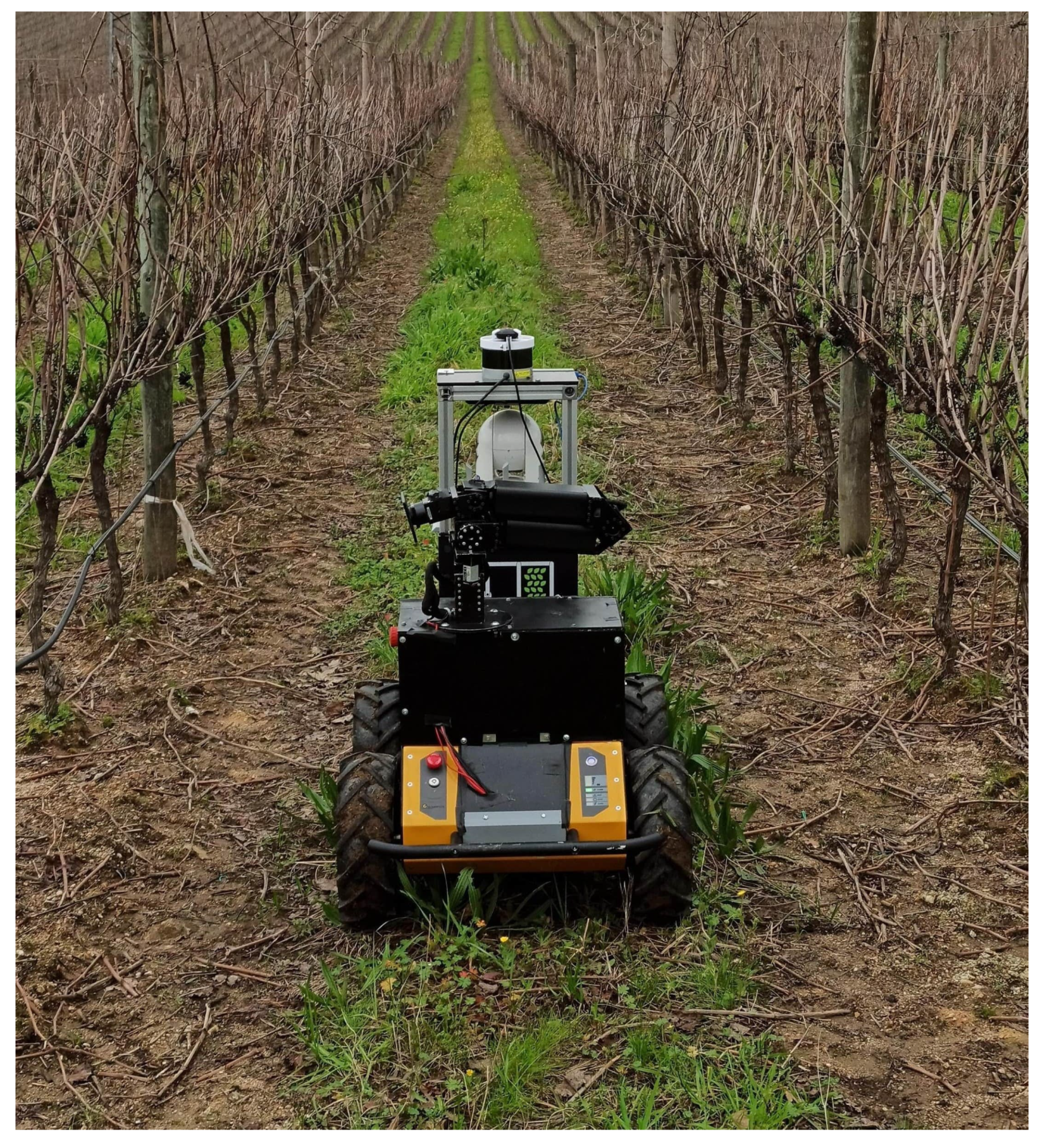
Figure 10 shows that occluded objects were taken into consideration during the annotation procedure and that the models were able to identify these objects in the images. Regarding the variations of the illumination conditions, one of the key steps to accomplish this goal was the capture of visual data during different days and stages of the year. To build the proposed dataset, the robot represented in
Figure 1 was taken four times to the vineyard in order to capture the crop state in different conditions. The visit dates were 11 May 2021, 27 May 2021, 23 June 2021, and 26 July 2021.
On each day, images were recorded both in the morning and during the evening to account for multiple light conditions. In May, grape bunches at an early growth stage were captured, while in June and July, the intermediate growth stage was present in the vineyard. After recording all these data, the annotation process was once again essential since during the annotation, the objects were present under different light conditions.
Figure 11 shows the different levels of illumination captured during the field visits performed. This figure proves that the models were able to detect grape bunches at different growth stages in these conditions.
4.3. Discussion
This work proposed a novel dataset for grape bunch detection at different growth stages. Two state-of-the-art models were used to perform this detection. Due to the requirement of a time-effective, low-power, and low-cost detection, this work used lightweight models that were quantized to be deployed in an embedded device. Quantization was used to reduce the size of the DL models and improve runtime performance by taking advantage of high throughput integer instructions. However, quantization can reduce the detection performance of DL models. Wu et al. [
51] showed that the error rates increase when the model size decreases by quantization. In this work, this decrease in detection performance was accepted due to the high gain in runtime performance. In comparison with state-of-the-art works such as the one proposed by Palacios et al. [
30], which detected grape flower at the bloom with an F1 score of 73.0%, this work presented a lower detection performance. On the other hand, the tradeoff between detection performance and runtime performance was extremely satisfactory since, especially for SSD MobileNet-V1, the model could perform with a mAP up to 66.96%, performing the detection at a rate higher than 10 Hz per image. In addition, the models were able to detect grape bunches at different stages, considering occlusions and variations in illumination conditions. Since the proposed dataset is publicly available, we believe that it has potential to be used in the future by the scientific community to train more complex and nonquantized DL models in order to achieve higher detection performances for applications without runtime restrictions. Furthermore, the proposed system can be adopted in future works and applications since it is cost-effective, portable, low-power, and independent of light conditions. The solution is modular and can be placed in any robotic platform, meaning that the price of the module is completely independent of the platform where it is placed. For applications that require higher levels of detection precision and that are not dependent on a time-effective solution, more complex models can be trained with the proposed dataset. Some works may also propose new DL-based architectures or modify state-of-the-art models to better suit the application purposes. For example, Taheri-Garavand et al. [
11] proposed a modification to the VGG16 model to identify chickpea varieties by using seed images in the visible spectrum, and Nasiri et al. [
12] proposed a similar approach to automate grapevine cultivar identification.
One of the main goals of this work was to achieve a low-power solution. The device used operates at high inference rate with a requirement of 5 V and 500 mA. This result was aligned with the state-of-the-art works that proposed advanced solutions for object detection using accelerator devices. Kaarmukilan et al. [
52] used Movidius Neural Compute Stick 2, which similar to the TPU used in this work, is connected to the host device by USB and is capable of 4 TOPS with a 1.5 W power consumption. Dinelli et al. [
53] compared several field-programmable gate array families by Xilinx and Intel for object detection. From all the evaluated devices, the authors achieved a minimum power consumption of 0.969 W and a maximum power consumption of 4.010 W.


