Sustainable Cotton Production through Increased Competitiveness: Analysis of Comparative Advantage and Influencing Factors of Cotton Production in Xinjiang, China

Abstract

Cotton production makes an important contribution to the income of rural residents and the economy in Xinjiang province, which leads other provinces in terms of planted area, total production, and average yield of cotton in China. This study analyzed the competitiveness of cotton production in the study area using the efficiency advantage index (EAI), scale advantage index (SAI), and aggregated advantage index (AAI). Moreover, the factors influencing the productivity of cotton have been investigated by the use of ridge regression and correlation matrix using a dataset for the period 2005 to 2018. The results showed that cotton production had a large comparative advantage in Xinjiang from 2005 to 2018. The average of efficiency advantage index (EAI), scale advantage index (SAI), and aggregated advantage index (AAI) are 1.50, 12.96, and 4.35, respectively. Overall, Xinjiang cotton production has a higher planting scale advantage and productivity. By using ridge regression to calculate the impact of cotton production on agricultural output value in Xinjiang, the results showed that total cotton production, fiscal expenditure on agricultural support, total agricultural machinery power, and fertilizer use had significant positive effects, whereas cotton sown area, average cotton yield, and the proportion of affected area by insects and diseases had negative impact agricultural output value. The study implies the need for a implementing a well-thought and empirically backed plan to support cotton production based on comparative advantage for a specific area, building a cotton production standard system, reducing the cost of cotton production, and building a cotton risk-protection system to protect the interests of cotton farmers and promote the sustainable development of the cotton industry.

1. Introduction

Cotton is one of the most important agricultural products in the world, and China is the world’s largest cotton importer and consumer and the second largest cotton producer [1]. Its domestic cotton demand and supply have a significant impact on the world market. Twenty-four of the 35 provinces of China grow cotton, with nearly 300 million people involved in cotton production [2]. Traditionally, cotton production in China was concentrated in the six provinces in the central and northern plains. In the past decade, cotton production had shifted to the Xinjiang province in the west, which has become the largest cotton producer in China [3]. Cotton production is important to economic growth in Xinjian. In 2020, China’s total cotton lint (deseed) output was 5.91 million tons, of which Xinjiang’s total cotton lint (deseed) output was 5.161 million tons, accounting for 87.33% of the country’s total output [4]. From 1995 to 2019, the cotton production in Xinjiang increased from 935,000 tons to 5,111,000 tons, with an average annual growth of 174,000 tons. Simultaneously, Xinjiang’s average cotton yield increased from 1.26 tons/ha to 2.05 tons/ha, and the per unit cotton yield in Xinjiang is 0.23 tons/ha higher than the national average yield in 2018 [5]. In summary, Xinjiang cotton and other major cotton-producing areas in China (Hebei Province, Shandong Province, Hubei Province, Anhui Province, Jiangxi Province, Hunan Province) have obvious production advantages in production, planting area, and yields.

David Ricardo’s “Theory of Comparative Advantage” believes that international trade arises from the difference in the opportunity cost of producing the product between countries, “Factor Endowment Theory” believes that international trade is generated because of the difference in factor endowment between countries, and “New Trade Theory” explains the origin of international trade from the perspective of economies of scale. The “new trade theory” explains the origin of international trade from the perspective of economies of scale [6,7,8,9,10,11].

Studies have been conducted to measure and evaluate the comparative advantage of crop regions, mainly from the selection and evaluation of evaluation indicators [12,13,14]. The evaluation indicators of the comparative advantages of crop areas can be generally divided into cost–benefit, comparative performance indicators, the domestic resource cost method, and the regional average cost method [15]. First of all, area and yield are the basic indicators for evaluating the comparative advantages of crop areas. Sown area and yield per unit area are applied in the study of the comparative advantage of maize, wheat, soybean, cotton, and peanut [16,17]. Second, some of the existing studies have added factors such as cost, return, and profit in evaluating the comparative advantages of regions [18]. Indicators such as production cost, land cost, land output ratio, output value, and net profit per unit have been used to reflect factors such as crop production costs, returns, and profits to comprehensively analyze the comparative advantage of crop industry development [19,20,21]. Third, the number of imports and exports, as well as the opportunity cost of labor and land, have also been introduced into the evaluation indexes by a small number of existing studies, mostly concerning the international competitiveness of products [22,23,24,25,26,27,28]. The methods for studying the comparative advantages of crop areas mainly include the integrated comparative advantage index method, the gray system assessment method, the engineering cost method, the equilibrium analysis method, the cost comparison method, and the price comparison method. The comprehensive comparative advantage index usually consists of scale, efficiency, and effectiveness comparative advantage indices, and is widely used in the study of the comparative advantages of food, which has both simplicity and science [29,30]. The domestic resource cost method, location entropy index method, correlation growth rate method, and data envelopment analysis method have also been applied in the study of comparative advantage [31].

This study involves the regional comparative advantage of cotton production and is based on the concept of comparative advantage in international trade theory and the analysis of cotton in Xinjiang in the region of a comprehensive comparison of relevant indicators, reflecting whether the production of cotton in Xinjiang has a comparative advantage, and it measures the size of the comparative advantage. Another purpose of this study is to provide a perspective on the determinants of agricultural output value by using regional data collected in Xinjiang. For this cross-sectional data, multilinear regression models are the most suitable approach [31]. Multicollinearity is one of the serious problems when using multiple linear regression at the macro level. This problem arises because of the high correlation between the independent variables, which leads to weak estimates [32].

Fisher [32] was the first researcher who found the seriousness of the multicollinearity problem and its effect on the results of the regression analysis. Hoerl and Kennard [33] added a positive value to the information matrix, which named the biased parameter and the ridge regression method. Montgomery and Peck [34] proved that the ridge trace depends on the path of the estimated curves versus several constant values between 0 and 1.

Wu et al., Hassan, et al., and Lee [35,36,37] found various reasons for the gross domestic product (GDP) to change and the economy to grow by using a large amount of theoretical and empirical research. Hasan et al. [37] found the factors of population, imports of goods and services, agricultural value-added, manufacturing value-added, and labor force have a positive impact on Bangladesh’s GDP through the comparison of stepwise and ridge regression models.

The overall objective of this study is to evaluate the comparative advantage of cotton production in Xinjiang province and the impact on the agricultural output value. Comparative advantage indexes, correlation analysis, and ridge regression techniques are used to build a plausible regression model. More specifically, the study (1) evaluate the comparative advantage of Xinjiang cotton production from 2005 to 2018, (2) analyze the correlation test between the independent and dependent variables using correlation analysis and multiple regression methods and determine the presence of multicollinearity between the variables with the inflation factor (VIF), and (3) analyze the magnitude of the factors influencing cotton production on agricultural output in Xinjiang using the ridge regression method to eliminate the multicollinearity between variables.

2. Materials and Methods

2.1. Study Area

The Xinjiang Uyghur Autonomous Region is located in the interior of the Eurasian continent and the northwestern part of China, with an area of about 1.66 × 100 km². It accounts for one-sixth of China’s land area and one-sixth of China’s national territory (Figure 1). Xinjiang has a typically arid continental climate with dry weather, large diurnal temperature difference, abundant heat resources, and the highest annual sunshine hours (2550–3500 h on average) in China. The climatic characteristics can effectively suppress the occurrence of cotton pests and diseases [36,37], which is suitable for high-quality cotton production [38]. Xinjiang has been the largest high-quality cotton growing base in China, with about 50% of farmers engaged in cotton production and 35% of their income related to cotton [39]. Currently, cotton production in Xinjiang is particularly important for further increasing farmers’ income, improving the livelihood of residents in ethnic areas, and promoting economic growth and sustainable agricultural development [40].

2.2. History of Cotton Cultivation in Xinjiang

Xinjiang has a long history of cotton cultivation and was one of the first regions to grow cotton in China. Before the 1980s, the area and total production of cotton in Xinjiang were low overall, accounting for only about 3% of the country [41]. Reforms and an opening-up promoted the rapid development of cotton production in Xinjiang. In the late 1980s and early 1990s, total cotton production and surface area in Xinjiang increased significantly. The increase in demand, technological upgrading, and policy support have contributed to the rapid development of the cotton industry in Xinjiang. Currently, Xinjiang ranks first in the country in terms of total cotton production and yields.

2.3. Data Collection

To analyze the comparative advantage of Xinjiang cotton production, data have been collected from the China Statistics Yearbook and Xinjiang Statistics Yearbook (1996–2020).

Considering the purpose of the study and the availability of data, this paper selects the cotton sown area, crop sown area of arable land, cotton yields, and total crop yield of arable land in China and Xinjiang from 2005 to 2019 as indicators to analyze the comprehensive comparative advantage of cotton production in Xinjiang. It is well-known that agricultural output is not only influenced by socioeconomic conditions but is also closely related to natural conditions. Drawing on existing studies [42], this paper selects agricultural output value (lnout) as the dependent variable indicator and total cotton production (lnpro) and cotton sown area (lnsown) as the core explanatory variables for Xinjiang from 1995 to 2020. In addition, cotton yield (lnyield), financial expenditure on agricultural support (lnfis), total agricultural machinery power (lnmac), fertilizer input quantity (lnfer), and the proportion of affected area to the adult area (lndis) were selected as control variables in this paper. The descriptive statistics of each variable are shown in

Table 1. Descriptive Statistics of Variables (1995–2019).

Variable	N	Min	Max	Mean	Std. Dev.
lnout	25	5.78	7.87	6.72	0.77
lnpro	25	4.54	6.24	5.43	0.51
lnfis	25	1.16	6.88	3.97	2.15
lnmac	25	6.48	7.93	7.21	0.49
lnfer	25	4.22	5.55	4.90	0.47
lnyield	25	7.07	7.78	7.42	0.18
lndis	25	3.73	4.37	4.06	0.18
lnsown	25	6.61	7.84	7.24	0.36

.

2.4. Comparative Advantage

This study quantify and analyze the comparative advantages of cotton production in Xinjiang relative to other major cotton producing regions (Hebei Province, Shandong Province, Hubei Province, Anhui Province, Jiangxi Province, and Hunan Province) in China from 2005 to 2019 by using three different indexes: efficiency advantage indices (EAI), scale advantage indices (SAI), and aggregate advantage indices (AAI) [43].

EAI is an indication of how efficiently a crop grows in one specific region. It is calculated by using the relative yield of one crop in one region related to the average yield of all crops in the same region to the yield of the same crop in the nation related to the average yield of all crops in the nation. EAI can be expressed as follows:

$$EA{I}_{ij}=\frac{Y_{ij}/Y_i}{Y_{nj}/Y_n}$$

(1)

where EAI_ij represents the efficiency advantage index of the jth crop growing in the ith region; Y_ij is the yield of the jth crop in the ith region; Y_i represents the average yield of all crops in the ith region; Y_nj is the national average yield of the jth crop; and Y_n is the national average yield of all crops. If EAI_ij > 1, the yield of the jth crop in the ith region, relative to all other crops’ yield growth in the same region, is higher than that of the national average. It can be interpreted that in the ith region there is a yield or an efficiency advantage in growing the jth crop. If EAI_ij < 1, the yield of the jth crop in the ith region, relative to all other crops’ yield growth in the same region, is lower than that of the national average. It can be interpreted that in the ith region there is no yield or efficiency advantage in growing the ith crop. By assuming a competitive market structure and no significant barriers to technology diffusion and adoption in agricultural production in the country, EAI_ij can be taken as an indicator of relative efficiency because of natural resource endowments and other local economic, social, and cultural factors.

The SAI indicates the extent of concentration of a certain crop growing in a region, relative to that ratio of the same crop growing in the nation. It can be expressed as follows:

$$SA{I}_{ij}=\frac{S_{ij}/S_i}{S_{nj}/S_n}$$

(2)

where SAI_ij is the scale advantage index of the jth crop in the ith region; S_ij represents the planted acreage of the jth crop in the ith region; S_i is the total planted acreage of all crops in the ith region; S_nj is the total planted acreage of the jth crop in the nation; and S_n represents the total planted acreage of all crops in the nation. If SAI_ij > 1, it implies the degree of concentration of the jth crop growing in the ith region is higher than the average concentration ratio in the nation. It also indicates that producers in the ith region prefer to grow a more jth crop, compared to other producers in the nation. If SAI_ij < 1, the degree of concentration of the jth crop growing in the ith region is lower than that average ratio in the nation. It indicates that producers in the ith region prefer to grow a less jth crop, compared to other producers in the nation.

Assuming a competitive market structure, those producers can quickly adjust the crop mix by responding to the market price and cost changes. Economic factors or the profit level of certain crop growth in the region determines the concentration level. For example, a low value of SAI_ij implies producers do not want to increase the share of that crop production in the region because it is less profitable or restricted by natural (or other) conditions, while a high value of SAI_ij implies producers want to increase the share of that crop production in the region.

The AAI is an indication of the overall comparative advantage of a certain crop in one region relative to the national average and can be calculated as the geometric average of the EAI and SAI.

$$AA{I}_{ij}=\sqrt{EA{I}_{ij}\ast SA{I}_{ij}}$$

(3)

If AAI_ij > 1, the jth crop in the ith region is considered to have an overall comparative advantage over the national average, while AAI_ij < 1 indicates jth crop in the ith region does not have an overall comparative advantage over the national average.

2.5. Correlation Analysis

Correlation analysis is a method of statistical evaluation used to study the strength of a relationship between two numerically measured, continuous variables. This particular type of analysis is useful in identifying possible connections among variables. If a correlation exists between two variables, it means that when there is a systematic change in one variable, there is also a systematic change in the other, or the variables alter together over a certain period [44].

In terms of the strength of the relationship, the value of the correlation coefficient varies between +1 and −1. A value of ±1 indicates a perfect degree of association between the two variables. As the absolute value of the correlation coefficient value goes toward 0, the relationship between the two variables is weaker. The direction of the relationship is indicated by the sign of the coefficient, where a + sign indicates a positive relationship and a −sign indicates a negative relationship. Usually, in statistics, four types of correlations are measured: the Pearson correlation, Kendall rank correction, Spearman correction, and point-biserial correction (Draper and Smith, 1998). The following formula is used to calculate the Pearson correlation:

$$r=\frac{N\sum xy-\sum x\sum y}{\sqrt{\left[N\sum x^2-{\left(\sum x\right)}^2\right]\left[N\sum y^2-{\left(\sum y\right)}^2\right]}}$$

(4)

where r is the Pearson correlation coefficient; N represents the number of observations; and x, y represent two variables.

To improve the accuracy of regression in this study, the Pearson correlation has been used to test the degree of correlation between the independent and independent variables. A high degree of autocorrelation between independent variables will affect the impact of independent variables on dependent variables.

2.6. Multiple Regression

Multiple linear regression (MLR) has been used to determine a mathematical relationship among several random variables. In other terms, MLR examines how multiple independent variables are related to the dependent variable. Once each of the independent variables has been determined to predict the dependent variable, the information on the multiple variables can be used to create an accurate prediction of the level of impact on the outcome variable. The model creates a relationship in the form of a straight line (linear) that best approximates all the individual data points. Multiple linear regression for cotton has an equation [45]:

lnOut = β₀ + β₁ lnpro + β₂ lnfis + β₃lnmac + β₄lnfer₊β₅ lnyield + β₆lndis + β₇lnsown + ε

(5)

where β₀, β₁, β₂, β₃, β₄, β₅, β₆, and β₇ are regression coefficients and ε represents a random error.

2.7. Ridge Regression

Cotton production is closely related to the economic development and rural residents’ income in Xinjiang. To model the agricultural output value of Xinjiang, seven variables are applied to predict the impact of cotton production on the agricultural output value of Xinjiang. Ridge regression is used to analyze the comprehensive effect of cotton production on agricultural output value in Xinjiang from 1995 to 2019. This study employed SAS 9.4 for statistical regression analysis.

2.7.1. Effects of Multicollinearity

Multicollinearity occurs when independent variables in a regression model are correlated. If the degree of correlation between independent variables is high enough, it can cause problems in fitting the model and interpreting the results. Multicollinearity can create inaccurate estimates of the regression coefficients, inflate the standard errors of the regression coefficients, deflate the partial t-tests for the regression coefficients and nonsignificant p-values, and degrade the predictability of the model [46].

2.7.2. Detection of Multicollinearity

There are several methods of detecting multicollinearity. In this study, two methods are used to test multicollinearity.

The variance inflation factor (VIF) is the ratio of variance in a model with multiple terms, divided by the variance of a model with one term alone. It quantifies the severity of multicollinearity in an ordinary least squares regression analysis. It provides an index that measures how much the variance (the square of the estimate’s standard deviation) of an estimated regression coefficient is increased because of collinearity (James et al., 2017). A VIF value greater than 10 indicates the presence of strong multicollinearity [47]. Snee [48] suggested that the VIF value should be below 5, and the independent variables will be uncorrelated if the VIF equals 1 [49].

The condition index is the standard measure of conditioning in a matrix. It indicates that the inversion of the matrix is numerically unstable with finite-precision numbers (standard computer floats and doubles). This indicates the potential sensitivity of the computed inverse to small changes in the original matrix. The condition number is computed by finding the square root of the maximum eigenvalue divided by the minimum eigenvalue of the design matrix. If the condition number is above 30, the regression can have significant multicollinearity. One advantage of this method is that it also shows which variables are causing the problem [50].

2.7.3. Ridge Regression Model

Ridge regression is a technique for analyzing multiple regression data that suffer from multicollinearity. When multicollinearity occurs, least squares estimates are unbiased, but the variances are large, so the result will be far from the true value. Adding a degree of bias to the regression estimates improves its explanatory power while the biased ridge regression is generally considered as the most popular method. Following the usual notation, suppose the regression equation is written in matrix form as:

$$Y=BX+e$$

(6)

where Y is the dependent variable; X represents the independent variables; $B$ is the regression coefficients to be estimated; and e represents the random error term.

In ordinary least squares, the regression coefficients are estimated using the formula:

$$\widehat{B}={\left(X^{\prime }X\right)}^{-1}{X}^{\prime }Y$$

(7)

As far as standardization is concerned, all ridge regression calculations are based on standardized variables. When the final regression coefficients are displayed, they are adjusted back to their original scale. However, the ridge trace is on a standardized scale. With the variables standardized, $X\prime X$ = R, where R is the correlation matrix of independent variables. These estimates are unbiased so that the expected value of the estimates are the population values. In Equation (8), $E\left(\widehat{B}\right)$ represents the unbiased estimator, $B$ represents the population value. That is:

$$E\left(\widehat{B}\right)=B$$

(8)

The variance inflation factors (VIF) measure the inflation of the parameter estimates being calculated for all independent variables in the regression model, as proposed by Donald and Glauber [51]. The VIF can be calculated as follows:

$$VIF=\frac{1}{1-R_j^2}\hspace{1em}\hspace{1em}j=0, 1, 2, \dots \dots , n$$

(9)

where $R_j^2$ is the coefficient of determination for the independent variables, the R_j² in the denominator gets closer to one and the variance (and VIF) will get larger.

The ridge regression proceeds by adding a small value k to the diagonal elements of the correlation matrix. That is:

$$\tilde{B}={\left(R+kI\right)}^{-1}{X}^{\prime }Y$$

(10)

where k is a positive quantity that ranges from 0 to 1 [52]. When k = 0, the results are the least square estimates. The amount of bias in this estimator is given by:

$$E\left(\tilde{B}-B\right)=[{\left(X^{\prime }X+kI\right)}^{-1}{X}^{\prime }X-I]B$$

(11)

and the covariance matrix is given by:

$$V\left(\tilde{B}\right)={\left(X^{\prime }X+kI\right)}^{-1}{X}^{\prime }X{\left(X^{\prime }X+kI\right)}^{-1}$$

(12)

One of the main obstacles in using ridge regression is in choosing an appropriate value of k. Hoerl and Kennard [53], the inventors of ridge regression, suggested using a graph, which can be called a ridge trace. This plot ridge can estimate regression coefficients as a function of k. When viewing the ridge trace, the analyst picks a value for k for which the regression coefficients have stabilized. Choose the smallest value of k as small as possible, after which the regression coefficients remain constant.

3. Results

3.1. Analysis of Comparative Advantage

According to Equation (1), EAI indicates the production efficiency of a crop in a particular region. As can be seen from Figure 2, from 2005 to 2018, an EAI greater than 1 means that the overall efficiency advantage of cotton production in Xinjiang is more obvious and shows a decreasing trend in the long term.

According to Equation (2), SAI indicates the scale efficiency advantage of a crop in a particular region. As can be seen from Figure 3, the SAI has increased from 10.47 to 19.70 from 2005 to 2018, implying that the scale efficiency advantage of cotton production in Xinjiang is obvious and shows an upward trend in the long term.

According to Equation (3), AAI indicates the overall comparative advantage of a crop relative to the national average. As can be seen from Figure 4, the AAI has been greater than 1 from 2005 to 2019, implying that the comprehensive comparative advantage of cotton production in Xinjiang is obvious and shows an upward trend in the long term.

Figure 5 indicates that cotton production in Xinjiang has obvious comprehensive advantages from 2005 to 2018. (1) The average SAI is 12.96, which means Xinjiang cotton has a higher scale advantage than other crops. From 2006 to 2009, cotton planted acreage in Xinjiang declined because of the global economic crisis. The SAI dropped from 10.47 to 9.11, which indicated the scale of cotton-planted acreage in Xinjiang was reduced by 34%. From 2015 to 2018, the SAI has the fastest growth with the implementation of the “Target Pricing” policy. (2) Compared to the SAI, EAI is affected by the yield factor. EAI is stable from 2005 to 2018, greater than 1, and the maximum value appears in 2015, reaching 1.74, indicating that the efficiency advantage of cotton in Xinjiang is very obvious. The average yield of cotton in Xinjiang is the highest in China. Climatic factors such as hail and drought will lead to fluctuations in output during the year. (3) The average value of AAI is 4.35, which means Xinjiang cotton has an overall comparative advantage and is higher than the national average in overall production. Figure 5 shows an increasing trend of AAI. It indicates Xinjiang cotton has a comparative advantage from 2005 to 2018.

3.2. Correlation between Variables

Table 2. Pearson Correlation Analysis.

Variable	lnout	lnpro	lnfis	lnmac	lnfer
lnout	1	0.953 **	0.930 **	0.989 **	0.992 **
lnpro	0.953 **	1	0.901 **	0.970 **	0.962 **
lnfis	0.930 **	0.901 **	1	0.925 **	0.940 **
lnmac	0.989 **	0.970 **	0.925 **	1	0.992 **
lnfer	0.992 **	0.962 **	0.940 **	0.992 **	1
lnyield	0.841 **	0.914 **	0.803 **	0.862 **	0.861 **
lndis	0.212	0.260	0.075	0.260	0.231
lnsown	0.927 **	0.982 **	0.868 **	0.948 **	0.944 **

** represents 99% confidence.

shows the Pearson correlation coefficients among the variables; the independent variables (Inpro, lnfis, lnmac, lnfer, lnyield, and lnsown) are highly correlated with the dependent variable out (agricultural output value) and with each other. The correlation coefficients are 0.8441 or above. In particular, the correlation coefficient between lnpro and lnsown is 0.982, the correlation coefficient between lnpro and Inmac is 0.970, and the correlation coefficient between lnmac and under is 0.992. Among the independent variables, the correlation coefficients are highly correlated with each another, which can cause multicollinearity and influence the accuracy of the estimated coefficients [54].

3.3. Multiple Regression

The independent variables require a collinear diagnosis before using Equation (5) for multiple regression analysis. The results are shown in

Table 3. Parameter Estimates.

Variable	DF	Parameter Estimate	Standard Error	T Value	Pr > |t|	Tolerance	Variance Inflation (VIF)
Intercept	1	2.198	2.785	0.789	0.441	–	–
lnpro	1	0.482	0.376	1.281	0.217	0.010	102.414
lnfis	1	−0.026	0.029	−0.873	0.395	0.091	11.043
lnmac	1	0.363	0.402	0.903	0.379	0.009	107.230
lnfer	1	1.428	0.395	3.617	0.002	0.010	96.051
lnyield	1	−0.404	0.306	−1.323	0.203	0.115	8.711
lndis	1	−0.082	0.132	−0.622	0.542	0.665	1.505
lnsown	1	−0.590	0.338	−1.745	0.099	0.024	41.296

and

Table 4. Collinearity Diagnostics.

Number	Eigenvalue	Condition	Proportion of Variation
		Index	Intercept	lnpro	lnfis	lnmac	lnfer	lnyield	lndis	lnsown
1	7.82	1.00	0.00	0.00	0.00	0.00	0.00	0.00	0.00	0.00
2	0.17	6.72	0.00	0.00	0.10	0.00	0.00	0.00	0.00	0.00
3	0.00	82.29	0.00	0.02	0.62	0.00	0.01	0.00	0.32	0.00
4	0.00	84.63	0.01	0.00	0.03	0.00	0.00	0.01	0.56	0.00
5	0.00	147.05	0.00	0.06	0.16	0.02	0.11	0.01	0.02	0.01
6	0.00	273.20	0.02	0.03	0.04	0.00	0.00	0.27	0.00	0.27
7	0.00	384.08	0.04	0.08	0.02	0.34	0.42	0.13	0.00	0.11
8	0.00	741.33	0.92	0.81	0.04	0.63	0.45	0.58	0.10	0.61

. The variance inflation factor (VIF) in Table 3 is a measure of multicollinearity. 0 < VIF < 5 indicates that multicollinearity is weak, while VIF ≥ 5 indicates a serious multicollinearity [55]. It can be seen that most VIFs in Table 3 are greater than 10, which means the independent variables have significant multicollinearity and require further statistical analysis.

Table 4 gives a collinearity diagnostics analysis of the independent variables. The condition index is 136.04, which is above 30 and indicates a multicollinearity problem in the data [50]. Meanwhile, the sum of the eigenvalues is equal to the number of independent variables. Eigenvalues near zero also indicate that there is multicollinearity in data. The eigenvalues represent the spread (variance) in the direction defined by the axis. Hence, small eigenvalues indicate the directions in which there is no spread. Since regression analysis seeks to find trends across values, when there is not a spread, the trends cannot be computed. There is a small eigenvalue (0.0003) in Table 4, which shows that there is a problem with collinearity in the independent variables.

Table 5. Analysis of Variance.

Source	DF	Sum of Squares	Mean Square	F Value	Pr > F
Model	7	14.126	2.018	233.79	<0.000
Residual	17	0.147	0.009
Total	24	14.272	0.595
Root MSE	0.092
R-Square	0.990
Adj R-Sq	0.986

shows the result of the analysis of variance. p-value is < 0.000 and F is 2233.79, revealing the significance of the regression model. The adjusted R-square is 0.986, which indicates the regression model fits well.

3.4. Results of Ridge Regression

To eliminate the influence of multicollinearity among the independent variables in Equation (5), ridge regression is used and the results are shown in

Table 6. The Parameter Estimates for the Ridge Regression.

Obs	_TYPE_	_RIDGE_	_RMSE_	Intercept	lnpro	lnfis	lnmac	lnfer	lnyield	lndis	lnsown	lnout
1	PARMS		0.09348	2.11687	0.467	−0.0248	0.355	1.4453	−0.4	−0.07367	−0.581	−1
2	RIDGEVIF	0			101.48	10.893	110.905	97.0921	8.424	1.5224	41.3796	−1
3	RIDGE	0	0.09348	2.11687	0.467	−0.0248	0.355	1.4453	−0.4	−0.07367	−0.581	−1
4	RIDGEVIF	0.01			17.363	7.5437	14.624	15.4518	4.842	1.29232	11.6042	−1
5	RIDGE	0.01	0.09917	−0.0876	0.2	0.003	0.662	0.982	−0.23	−0.08464	−0.2481	−1
6	RIDGEVIF	0.02			7.925	5.9428	7.054	7.5194	4.062	1.21217	7.1054	−1
7	RIDGE	0.02	0.10529	−0.4843	0.173	0.0172	0.659	0.851	−0.19	−0.07124	−0.1393	−1
8	RIDGEVIF	0.03			4.697	4.8642	4.504	4.7345	3.574	1.1526	5.1572	−1
9	RIDGE	0.03	0.11115	−0.7005	0.169	0.0268	0.634	0.7732	−0.16	−0.05999	−0.0706	−1
10	RIDGEVIF	0.04			3.174	4.0845	3.236	3.3528	3.203	1.10376	4.0361	−1
11	RIDGE	0.04	0.1165	−0.866	0.171	0.0337	0.607	0.7181	−0.14	−0.0513	−0.0208	−1
12	RIDGEVIF	0.05			2.323	3.496	2.481	2.5412	2.9	1.06195	3.2965	−1
13	RIDGE	0.05	0.12133	−1.0085	0.173	0.039	0.583	0.6759	−0.11	−0.04468	0.0175	−1
14	RIDGEVIF	0.05			2.323	3.496	2.481	2.5412	2.9	1.06195	3.2965	−1
15	RIDGE	0.05	0.12133	−1.0085	0.173	0.039	0.583	0.6759	−0.11	−0.04468	0.0175	−1
16	RIDGEVIF	0.06			1.793	3.0373	1.984	2.0139	2.645	1.0252	2.7685	−1
17	RIDGE	0.06	0.12566	−1.1377	0.177	0.043	0.561	0.6422	−0.09	−0.03947	0.0481	−1
18	RIDGEVIF	0.07			1.437	2.6708	1.634	1.6474	2.426	0.9923	2.3716	−1
19	RIDGE	0.07	0.12957	−1.2571	0.18	0.0462	0.542	0.6143	−0.07	−0.03531	0.0732	−1
20	RIDGEVIF	0.08			1.185	2.3722	1.376	1.3802	2.235	0.96242	2.0625	−1
21	RIDGE	0.08	0.1331	−1.3682	0.183	0.0488	0.525	0.5907	−0.04	−0.03193	0.0941	−1
22	RIDGEVIF	0.09			0.999	2.1249	1.18	1.1781	2.067	0.93502	1.8151	−1
23	RIDGE	0.09	0.13633	−1.4721	0.186	0.0509	0.51	0.5705	−0.02	−0.02911	0.1118	−1
24	RIDGEVIF	0.1			0.858	1.9172	1.025	1.0209	1.919	0.90965	1.6131	−1
25	RIDGE	0.1	0.13929	−1.5694	0.188	0.0525	0.496	0.5528	−0.01	−0.02672	0.127	−1
26	RIDGEVIF	0.2			0.311	0.8838	0.39	0.3862	1.044	0.72315	0.6794	−1
27	RIDGE	0.2	0.16023	−2.2715	0.204	0.0596	0.413	0.4494	0.136	−0.01273	0.2091	−1
28	RIDGEVIF	0.3			0.173	0.5251	0.218	0.2168	0.663	0.60015	0.3848	−1
29	RIDGE	0.3	0.17382	−2.6605	0.21	0.0605	0.37	0.3996	0.221	−0.0035	0.2411	−1
30	RIDGEVIF	0.4			0.116	0.3552	0.145	0.145	0.462	0.50944	0.2526	−1
31	RIDGE	0.4	0.18459	−2.8796	0.213	0.0601	0.343	0.3687	0.276	0.00473	0.2567	−1
32	RIDGEVIF	0.5			0.087	0.2603	0.107	0.1073	0.342	0.43916	0.1816	−1
33	RIDGE	0.5	0.19404	−2.9983	0.213	0.0591	0.324	0.3469	0.313	0.01226	0.2648	−1

and Figure 2 for the four independent variables.

It can be seen that in Table 6, when k close is to 0.04, the ridge trace curve tends to be stable, and all VIFs are between 0 to 5, which indicates the multicollinearity between variables has been eliminated [49]. Similarly, root means square error (RMSE) is the standard deviation of the residuals (prediction errors). If the RMSE is smaller, then the regression results are better [56].

Figure 6 shows the ridge trace for agricultural output value with the standardized regression coefficients on the vertical axis and various values of k on the horizontal axis. The objective of the ridge regression analysis is to determine the best value of k when these coefficients are stable. In this study, the value of k is determined in the range of 0.00 to 0.50; the value selected on this graph happens to be 0.04, the value obtained from the analysis results.

When k = 0.04, (Table 6) multicollinearity is eliminated and the estimated regression equation is (Table 6):

$$\ln out=-0.87+0.17lnpro+0.03 lnfis+0.61 lnmac+0.72lnfer-0.14lnyield-0.05lndis-0.02lnsown$$

(13)

The regression coefficients of the independent variables in Equation (13) reflect that for each percentage increase in total cotton production, the agricultural output value increases by 0.17%; for each percentage increase in financial support for agriculture, the agricultural output value increases by 0.03%; for each percentage increase in total agricultural machinery power, agricultural output value increases by 0.61%; and for each percentage increase in fertilizer input, agricultural output value increases by 0.72%. In contrast, cotton yields, the proportion of disaster area, and cotton sown area harmed agricultural output. In particular, the agricultural output value decreased by 0.14% for each percentage increase in cotton yield, by 0.05% for each percentage increase in the proportion of affected area to the adult area and by 0.02% for each percentage increase in cotton sown area. The increase in the area of disaster in agriculture will directly affect the increase in agricultural output.

4. Conclusions and Discussion

4.1. Conclusions

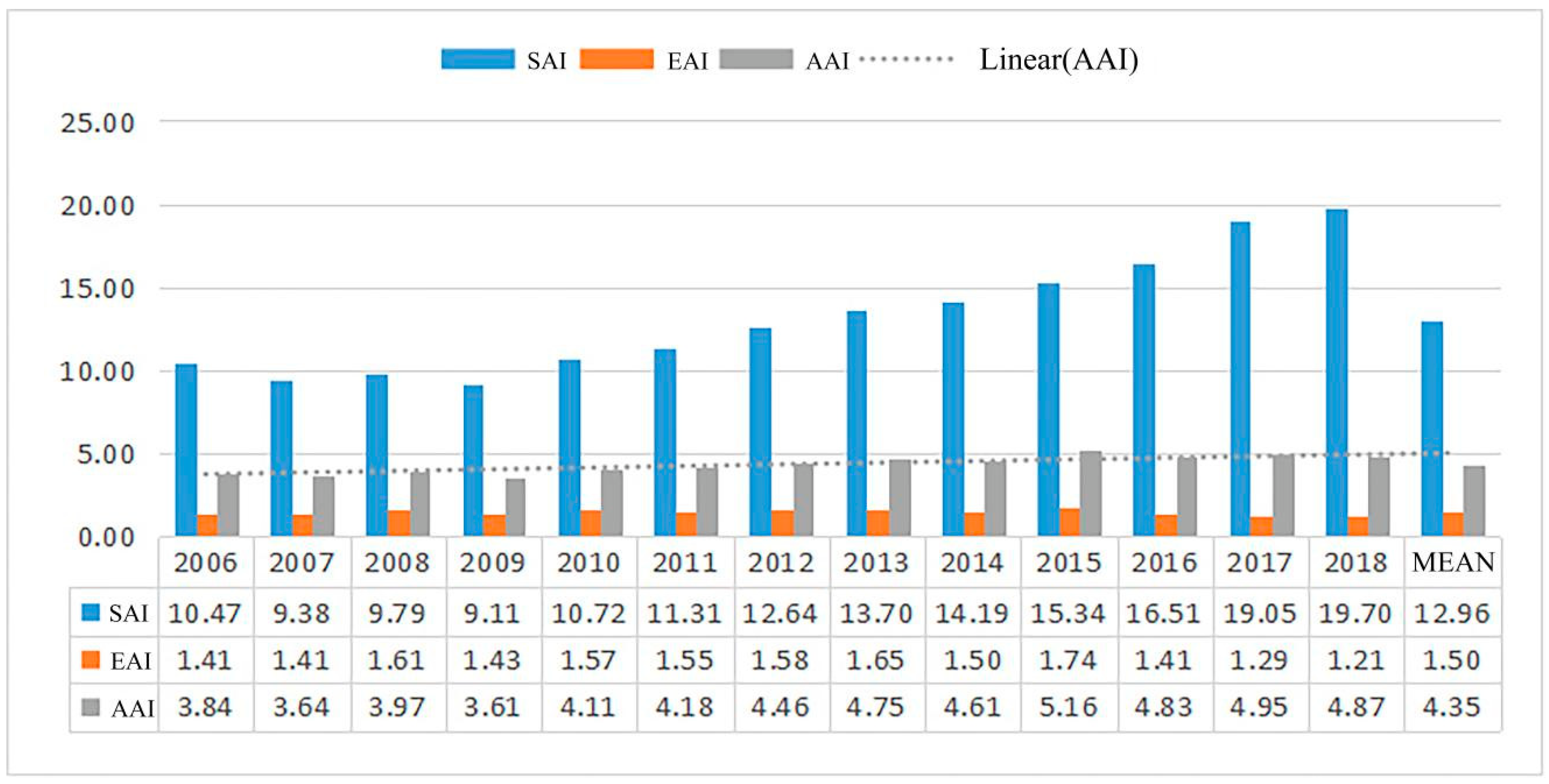
Cotton production in Xinjiang makes a significant contribution to the Chinese and world cotton markets. It ranks first in China in terms of planted area, total production, and average yield. Three different indices were calculated in this study, the efficiency advantage index (EAI), scale advantage index (SAI), and aggregate advantage index (AAI), to evaluate the comparative advantage of cotton production in Xinjiang. Second, this study applied correlation, multiple linear regression, and ridge regression to analyze the effect of cotton production in Xinjiang and its impact on agricultural output.

(1) The comparative advantage of cotton production in Xinjiang is obvious. By calculating the efficiency advantage index (EAI), scale advantage index (SAI), and comprehensive advantage index (AAI) of cotton production in Xinjiang from 2005 to 2018, the results show that cotton production in Xinjiang has obvious comparative advantages. The average values of SAI, EAI, and AAI are 12.96, 1.50, and 4.35, respectively, indicating that cotton production in Xinjiang has a high planting scale advantage and yield advantage.

(2) The results of the analysis of the factors affecting the agricultural output value of cotton production in Xinjiang show that agricultural output value and cotton production have a high correlation. Ridge regression analysis shows that total cotton production, financial support for agricultural expenditure, total agricultural machinery power, and fertilizer use have significant positive effects on agricultural output value in Xinjiang. Cotton planting area, average cotton yield, and the proportion of affected area, on the other hand, had a negative effect on the agricultural output value.

4.2. Discussion

(1) The scale advantage of cotton production in Xinjiang is very obvious, mainly because of the large cotton sowing area in Xinjiang, which reached 375.996 million mu in 2021, accounting for 82.76% of the national planting area [57], and the full mechanization of cotton production in Xinjiang from sowing to harvesting, which further promotes the scale of cotton production. This result is important for policymakers, who should develop a more optimal scale of cotton cultivation in Xinjiang to ensure that the sustainable development of cotton production is coordinated with the environmental carrying capacity.

(2) The comparative advantage of cotton efficiency in Xinjiang shows a trend of a slow growth rate; as the overall level of cotton yield in Xinjiang is high, its marginal yield increase space becomes smaller, and the future single increase relies on variety improvement and technology improvement.

(3) Fertilizer application has an obvious positive effect on the agricultural output value; considering that agricultural production in Xinjiang is constrained by resources and the environment, the use of fertilizer needs to be gradually reduced in the future, while the area affected by disasters has a negative effect on agricultural output value, and agricultural infrastructure construction needs to be strengthened to improve the disaster resistance of agricultural production.

4.3. Policy Recommendations

Under the influence of multiple factors, for Xinjiang cotton production to maintain a sustained high yield, there is a need to overcome difficulties in the cotton production faced in recent years along with emphasizing the need to enhance planting scale and per unit yield. Due to the impact of international cotton prices and costs, the total production of cotton in Xinjiang is high, but the quality of cotton is poor, resulting in the international competitiveness of cotton not being strong. In view of this, for the establishment of a new concept of high-quality sustainable development of the cotton industry, and adjusting the cotton security strategy, it is recommended that the following four aspects reshape the economy of the cotton industry in Xinjiang, consolidating and enhancing the comparative advantage of cotton production, to ensure the security of cotton production.

4.3.1. Reasonable Planning of the Layout of the Cotton Industry

Based on in-depth investigation and research, the overall planning of the cotton industry in Xinjiang requires a scientific layout, the establishment of several high-yielding, stable production fields, and a high-quality cotton production base; under the premise of safeguarding the security of the national cotton industry, the appropriate adjustment of cotton planting area, according to local conditions. It also, requires a reasonable development of agricultural resources and the reshaping of agricultural enterprises throughout Xinjiang, so that Xinjiang’s agricultural structure changes from single to diversified entity [58]. The optimization and integration of the cotton industry chain in Xinjiang requires the promotion of cotton seed breeding; planting, acquisition, and processing as well as cotton spinning by placing them under one industrialized management system, and the formation of a complete cotton industry chain for achieving economies of scale and competitive edge both locally and internationally.

4.3.2. Building Cotton Seed Monitoring and Quality Standard System

Establishing and improving seed-quality monitoring while setting up special seed management departments to ensure that seed inspection works perfectly. It also requires to improve the technical level of seed-quality testing standards, mainly to ensure the purity and varietal integrity of seeds while promoting the application of DNA molecular marker technology and protein gel electrophoresis technology. Similarly, there is a need to pay attention to crop seed DNA and protein testing, and establishing the corresponding seed database; improving the quality of management personnel, and regularly organizing relevant management personnel to participate in training and assessment to enhance the level of seed management. [59]. By building a standardized system for cotton production, implementing standardized primary processing and improving cotton quality standards and cotton seed monitoring system, we can solve the problem of mixed heterogeneous fibers in Xinjiang cotton from the source and improve the core competitiveness of Xinjiang cotton. Another aspect relates to guiding cotton farmers to participate in cotton quality production process and raising their awareness on quality production and safety through training by cooperatives and agricultural technology companies.

4.3.3. Reducing the Cost of Cotton Production

Sustainable production of cotton requires establishing a long-term mechanism to develop machine-picked cotton and providing subsidy like being applied to the current food standards, thus encouraging cotton farmers to produce better lint and seed cotton through subsidized inputs [60]. Developing preferential support policies in finance, credit, insurance, taxation, and comprehensive subsidies for agricultural production materials to vigorously support cotton production in Xinjiang are also needed to reduce production costs. At the same time, with the railway department to maintain timely communication and coordination, from October of each year to February of the following year, the peak period of cotton in Xinjiang, increasing the number of empty wagons in Xinjiang for special cotton transport to achieve efficient docking of cotton production and consumption can be pivotal for development of cotton economy.

4.3.4. Construction of Cotton Risk-Protection System

Natural climatic conditions in Xinjiang are harsh and natural disasters are frequent, directly causing losses in cotton production and reduced income for cotton farmers. Therefore, a comprehensive agricultural insurance mechanism for cotton production was established to guarantee the sustainable development of the cotton industry in Xinjiang [61]. At the same time, the dramatic price fluctuations of cotton also seriously restrict the development of the cotton industry in Xinjiang. Combined with the current implementation of the “insurance + futures” pilot work in Xinjiang cotton, the future of the cotton industry in Xinjiang in response to natural risks and market risks, the establishment of early warning mechanisms to protect cotton farmers’ income is the key to the sustainable, healthy, and stable development of the cotton industry in Xinjiang [62], relying on cooperative finance, withdrawing catastrophe risk funds, and adopting mutual assistance of farmers to cope with production risks.

4.4. Limitations of the Study and Future Research

Recommendations for future research include, first, that additional data encompassing a larger region and covering multiple years would enhance the representativeness of the findings. Second, the study would include more variables to analyze the impact on agricultural output value (cost, policy, modern technology, etc.). Third, future research should include an in-depth analysis of the influence of cotton production in Xinjiang on China and the world cotton market. Nonetheless, despite the foregoing recommendations for future research, the present analysis is a solid contribution to the impact of cotton production on the agricultural output value in Xinjiang, China.

References

1. Lei, W.; Ben, F. Analysis of the competitiveness of the cotton industry in Xinjiang based on the diamond model. UTMS J. Econ. 2021, 12, 123–146. Available online: https://ideas.repec.org/a/ris/utmsje/0311.html (accessed on 12 July 2022).
2. Zhang, J. Study on the ways to realize the High-quality Development of bingtuan Cotton Industry under the background of regiment Farm Reform. Xinjiang State Farms Econ. 2022, 5, 93. Available online: https://kns.cnki.net/kcms/detail/detail.aspx?dbcode=CJFD&dbname=CJFDLAST2022&filename=NONG202205011 (accessed on 12 July 2022).
3. Yang, Z.; Tang, J.; Yu, X. Xinjiang Cotton Industry Present Situation and Countermeasure Research. Res. Agric. Mod. 2013, 34, 298–302. Available online: https://kns.cnki.net/kcms/detail/detail.aspx?dbcode=CJFD&dbname=CJFD2013&filename=NXDH201303011 (accessed on 12 July 2022).
4. National Bureau of Statistics of China. Available online: http://www.stats.gov.cn/english/ (accessed on 12 July 2022).
5. Statistical Bureau of Xinjiang Uygur Autonomous Region. Statistical Yearbook of Xinjiang; China Statistics Press: Beijing, China, 2020.
6. Zhong, F.; Xu, Z.; Fu, L. Regional Comparative Advantage in China’s Main Grain Crops. 2001. Available online: https://openresearch-repository.anu.edu.au/handle/1885/40535 (accessed on 12 July 2022).
7. Zhang, S.Y. Research on Comparative Advantage and Production Layout of Oilseed Crops in China. Huazhong Agricultural University. 2005. Available online: https://kns.cnki.net/kcms/detail/detail.aspx?dbcode=CDFD&dbname=CDFD9908&filename=2005153605.nh (accessed on 12 July 2022).
8. Yin, X.; Dong, N. Analysis of comparative advantages of peanut production in Shandong Province. Rural Econ. Technol. 2014, 25, 53–54. [Google Scholar] [CrossRef]
9. Liang, S. Analysis on the Comparative Advantages of Regional Special Agricultural Products in Hebei Province. J. Agric. Tech. Econ. 2008, 6, 91–94. Available online: https://kns.cnki.net/kcms/detail/detail.aspx?dbcode=CJFD&dbname=CJFD2008&filename=NYJS200806013 (accessed on 12 July 2022).
10. Liang, Y. Research on the International Competitiveness of Henan Province’s Agricultural Export Trade and Its Influencing Factors.HenanAgriculturalUniversity2014. Available online: https://kns.cnki.net/kcms/detail/detail.aspx?dbcode=CMFD&dbname=CMFD201501&filename=1014420936.nh (accessed on 12 July 2022).
11. Yu, X.; Yu, M.; Ewell, F. The Comparative Advantage of Upland Cotton Production in Texas. Tex. J. Agric. Nat. Resour. 2006, 19, 31–38. Available online: https://txjanr.agintexas.org/index.php/txjanr/article/view/109 (accessed on 12 July 2022).
12. Xu, S. Research on Comparative Advantages and Market Competitiveness of Corn Production in Jilin Province. China Agricultural University. 2004. Available online: https://kns.cnki.net/kcms/detail/detail.aspx?dbcode=CMFD&dbname=CMFD9904&filename=2004078059.nh (accessed on 12 July 2022).
13. Chen, Q.; Yang, Z.; Li, Q. Spatial and Temporal Distribution Characteristics of Corn Comparative Advantage in Beijing-Tianjin-Hebei region. Anhui Agric. Sci. 2018, 46, 4–8. [Google Scholar] [CrossRef]
14. Lv, J.; Xi, X.; Liu, H.; Han, X.; Jiang, F. Study on the change of maize layout and its regional comparative advantage in Liaoning Province. J. Shenyang Agric. Univ. 2016, 47, 379–384. [Google Scholar] [CrossRef]
15. Cui, Q.; Zhou, N.; Sun, C. Analysis of the contribution rate and regional comparative advantage of grain production in main production areas: Rice, wheat, and corn as examples. Agric. Econ. Manag. 2013, 2, 35–42. [Google Scholar] [CrossRef]
16. Li, M.; Zhou, Y.; Zhou, L.; Yang, J.; Wang, Y. Evolution of regional dominance of wheat production in China and analysis of driving factors. China Agric. Resour. Zoning 2015, 36, 7–15. [Google Scholar] [CrossRef]
17. Wang, X. Comparison of regional advantages of major grain varieties production in China. Financ. Econ. Sci. 2014, 7, 102–113. [Google Scholar] [CrossRef]
18. Zhao, F. Analysis of comparative advantages of corn production in China. Res. Financ. Econ. 2010, 8, 48–51. [Google Scholar] [CrossRef]
19. Li, M.; Wang, Y.; Liu, X.; Li, Y.; Zhang, Y.; Zhou, Y.; Wang, J. Analysis of corn production trade and comparative advantage between China and the United States—Based on the perspective of cost-effectiveness and productivity. Maize Sci. 2013, 21, 138–142+147. [Google Scholar] [CrossRef]
20. Yu, L.; Mu, Y. Research on the comparative advantage of maize production regions in China. Anhui Agric. Sci. 2017, 45, 236–239. [Google Scholar] [CrossRef]
21. Xu, C. Comparative Advantage and the Restructuring of Agricultural Production in China. Nanjing Agricultural University. 2001. Available online: https://kns.cnki.net/KCMS/detail/detail.aspx?dbname=CDFD9908&filename=2001012856.nh (accessed on 12 July 2022).
22. Carter, C.; Zhong, F. Will market prices enhance Chinese agriculture?: A test of regional comparative advantage. West. J. Agric. Econ. 1991, 16, 417–426. Available online: https://www.jstor.org/stable/40982765 (accessed on 12 July 2022).
23. Greenaway, D.; Hassan, R.; Reed, G. An empirical analysis of comparative advantage in Egyptian agriculture. Appl. Econ. 1994, 26, 649–657. [Google Scholar] [CrossRef]
24. Masters, W.; Winter, N.; Nelson, A. Measuring the Comparative advantage of agricultural activities: Domestic resource costs and the social cost-benefit ratio. Am. J. Agric. Econ. 1995, 77, 243–250. [Google Scholar] [CrossRef]
25. Li, Q.; Li, X. Measurement of comparative advantage of agricultural products in Liaoning. J. Dalian Marit. Univ. (Soc. Sci. Ed.) 2014, 13, 14–21. [Google Scholar] [CrossRef]
26. Xu, Z.; Zhang, S.; Ma, R.; Qiu, H. A comparison of the advantages of corn industry development between China and the United States in the context of bioenergy development—Based on the comparative advantage analysis of land output rate and production cost. Agric. Econ. Manag. 2010, 6, 8–14+40. [Google Scholar] [CrossRef]
27. Mei, N.; Sun, L. Research on the competitiveness and comparative advantage of China’s corn trade. Econ. Vert. 2014, 11, 67–70. [Google Scholar] [CrossRef]
28. Fert, I.; Hubbard, L. Revealed comparative advantage and competitiveness in Hungarian agri-food sectors. World Econ. 2003, 26, 247–259. [Google Scholar] [CrossRef]
29. Jiang, J.; An, X.; Wang, Y.; Du, Y. Model analysis of regional comparative advantage of maize production in China. Agric. Mod. Res. 1998, 1, 9–12. Available online: https://kns.cnki.net/kcms/detail/detail.aspx?dbcode=CJFD&dbname=CJFD9899&filename=NXDH801.002 (accessed on 12 July 2022).
30. Corden, W.M. Trade Policy and Economic Welfare; Clarendon Press: Oxford, UK, 1974. [Google Scholar]
31. Appleyard, D. Comparative Advantage of Agriculrural Production Systems and Its Policy Implications in Pakistan; Development Paper No. 68; Food and Agriculture Organization: Rome, Italy, 1987. [Google Scholar]
32. Fisher, R.A. Probability likelihood and quantity of information in the logic of uncertain inference. Proc. R. Soc. Lond. A 1934, 146, 1–8. [Google Scholar] [CrossRef]
33. Hoerl, A.E.; Kennard, R.W. Ridge Regression: Biased Estimation for No orthogonal Problems. Technometrics 1970, 1, 69–82. [Google Scholar] [CrossRef]
34. Montgomery, D.C.; Peck, E.A. Introduction to Linear Regression Analysis; John Wiley and Sons: New York, NY, USA, 1982. [Google Scholar]
35. Wu, S.; Tang, J.H.; Lin, E.S. The impact of government expenditure on economic growth: How sensitive to the level of development? J. Policy Modeling 2010, 32, 804–817. [Google Scholar] [CrossRef]
36. Lee, J. Export specialization and economic growth around the world. Econ. Syst. 2011, 3, 45–63. [Google Scholar] [CrossRef]
37. Hasan, M.N.; Sohel, R.; Malek, M.B.; Das, K.R.; Sultana, N. Modeling Bangladesh’s Gross Domestic Product Using Regression Approach. Malays. J. Math. Sci. 2016, 10, 233–246. Available online: https://www.semanticscholar.org/paper/Modeling-Bangladesh’s-gross-domestic-product-using-Hasan-Rana/85eff8d6eb3a27ceb653b10719d770e13e4fc4f4 (accessed on 12 July 2022).
38. Li, N.; Li, Y.; Biswas, A.; Wang, J.; Dong, H.; Chen, J.; Liu, C.; Fan, X. Impact of climate change and crop management on cotton phenology based on statistical analysis in the main-cotton-planting areas of China. J. Clean. Prod. 2021, 298, 126750. [Google Scholar] [CrossRef]
39. Ma, C.; Mamat, S.; Yao, J.; Gulnur, I. Spatial and temporal dynamics of cotton production in China from 1950–2015. J. Geogr. 2020, 75, 1699–1710. [Google Scholar] [CrossRef]
40. Wang, J.; Liang, Y.J.; Gong, Z.L.; Ai, X.T.; Li, X.Y.; Zheng, J.Y. Comparison of costs and benefits and advantages of cotton production in China, USA, and Australia. Cotton Sci. 2016, 38, 13–18. [Google Scholar] [CrossRef]
41. Du, M. Analysis of constraints and development prospects of cotton production in China. World Agric. 2017, 11, 223–226. [Google Scholar] [CrossRef]
42. Will, J. Some support policy options for cotton in China. China Agric. Econ. Rev. 2008, 1, 23–37. [Google Scholar] [CrossRef]
43. Zhou, S.; Jing, L.; Meng, H.; Qiao, H. Evolution of production layout patterns and motives of peanut production in China’s main production areas. Agric. Technol. Econ. 2018, 3, 100–109. Available online: https://kns.cnki.net/kcms/detail/detail.aspx?dbcode=CJFD&dbname=CJFDLAST2018&filename=NYJS201803009 (accessed on 12 July 2022).
44. Xu, T.; Meng, T.; Mu, Y. Comparative advantages of provincial maize production in China and its influencing factors—Empirical evidence based on panel data of 20 main maize producing areas from 2008–2017. J. China Agric. Univ. 2020, 25, 102–111. Available online: https://kns.cnki.net/kcms/detail/detail.aspx?dbcode=CJFD&dbname=CJFDLAST2020&filename=NYDX202006012 (accessed on 12 July 2022).
45. Ma, H. Theoretical Research and Empirical Analysis on Comparative Advantage of Regional Agricultural Products. Xinjiang Agricultural University. 2004. Available online: https://kns.cnki.net/KCMS/detail/detail.aspx?dbname=CDFD9908&filename=2004118718.nh (accessed on 12 July 2022).
46. Kendall, M.; Gibbons, J. Rank Correlation Methods, 5th ed.; Edward Arnold: London, UK, 1990. [Google Scholar]
47. Zhu, J.; Cui, D. The evolution of cotton purchase and sale system in Xinjiang Corps and the behavior of main interests and countermeasures suggestions. Agric. Mod. Res. 2012, 33, 603–606. [Google Scholar] [CrossRef]
48. Foster, J. Multi-collinearity in Regression Analysis: Problems, Detection, and Solutions. 2017. Available online: http://statisticsbyjim.com/regression/multicollinearity-in-regression-analysis/ (accessed on 14 February 2018).
49. Marquardt, D. The Importance of Statisticians. J. Am. Stat. Assoc. 1987, 82, 1–7. [Google Scholar] [CrossRef]
50. Snee, D. Some Aspects of No orthogonal Data Analysis. Part I. Developing Prediction Equation. J. Qual. Technol. 1973, 5, 67–79. [Google Scholar] [CrossRef]
51. Levine, D.; Krehbiel, T.; Berenson, M. Business Statistics: A First Course, 3rd ed.; Prentice Hall: Hoboken, NJ, USA, 2003. [Google Scholar]
52. Belsley, D. A guide to using the collinearity diagnostics. Comput. Sci. Econ. Manag. 1991, 4, 33–50. [Google Scholar] [CrossRef]
53. Donald, E.; Glauber, R. Multi-collinearity in Regression Analysis: The Problem Revisited. Rev. Econ. Stat. 2011, 49, 92–107. [Google Scholar] [CrossRef]
54. Brown, P.; Payne, C. Election Night Forecasting. J. R. Stat. Soc. Ser. A 1975, 138, 463–483. [Google Scholar] [CrossRef]
55. Hoerl, A.; Kennard, R. Ridge regression: Iterative estimation of the biasing parameter. Commun. Stat. Theory Method 1976, 5, 77–88. [Google Scholar] [CrossRef]
56. National Bureau of Statistics Explains Cotton Production in 2021. Available online: http://www.gov.cn/shuju/2021-12/14/content_5660706.htm/ (accessed on 14 December 2021).
57. Introduction to Ridge Regression. 2020. Available online: https://www.statology.org/ridge-regression/ (accessed on 11 November 2020).
58. RMSE: Root Mean Square Error. 2018. Available online: http://www.statisticshowto.com/rmse/ (accessed on 27 February 2018).
59. Dave, D. Comparative advantage and agricultural trade. Agric. Econ. 2019, 50, 29–40. [Google Scholar] [CrossRef]
60. Pan, X.; Li, K. GIS-based analysis of spatial and temporal variability of cotton production development in Xinjian. Geogr. Arid. Reg. 2000, 3, 199–206. [Google Scholar] [CrossRef]
61. Natalia, I.; Lubos, S. Revealed comparative advantage of Russian agricultural exports. Acta Univ. Agric. Silvic. Mendel. Brun. 2013, 61, 941–952. [Google Scholar] [CrossRef]
62. Li, H.; Zhou, S. Analysis of competitive market advantages of cotton production in Xinjiang. Agric. Technol. Econ. 2007, 3, 96–101. [Google Scholar] [CrossRef]
Figure 1. Study area map in Xinjiang.
Agronomy 12 02239 g001
Figure 2. Xinjiang cotton production efficiency advantage (EAI).
Agronomy 12 02239 g002
Figure 3. Xinjiang cotton production scale advantage (SAI).
Agronomy 12 02239 g003
Figure 4. Xinjiang cotton production comprehensive comparative advantage (AAI).
Agronomy 12 02239 g004
Figure 5. Comparative advantage of Xinjiang cotton production from 2005–2018.
Agronomy 12 02239 g005
Figure 6. Ridge trace for the agricultural output value.
Agronomy 12 02239 g006