

Multiple Stresses of Wheat in the Detection of Traits and Genotypes of High-Performance and Stability for a Complex Interplay of Environment and Genotypes
 , and
, and 
Abstract
:1. Introduction
2. Materials and Methods
2.1. Genotypes and Experimental Design
2.2. Measurements and Data Collection
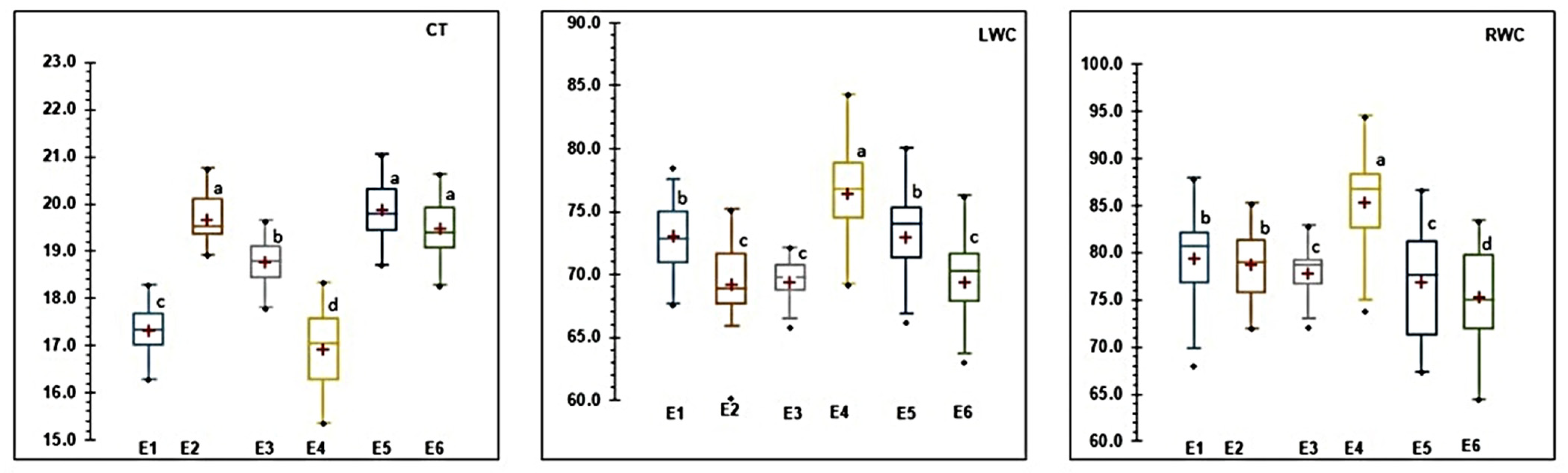
2.2.1. Morpho-Physiological Parameters
2.2.2. Agronomic and Yield Trait Parameters
2.3. Statistical Analysis
2.3.1. Analysis of Variance
2.3.2. Stepwise Multiple Linear Regression Analysis (SMLRA)
2.3.3. GEI Analysis
AMMI Analysis
GGE Biplot
2.4. Statistical Software
3. Results
3.1. ANOVA and Mean Performances of 20 Genotypes
3.2. Identification of Traits Associated with Grain Yield
3.3. GEI Analysis
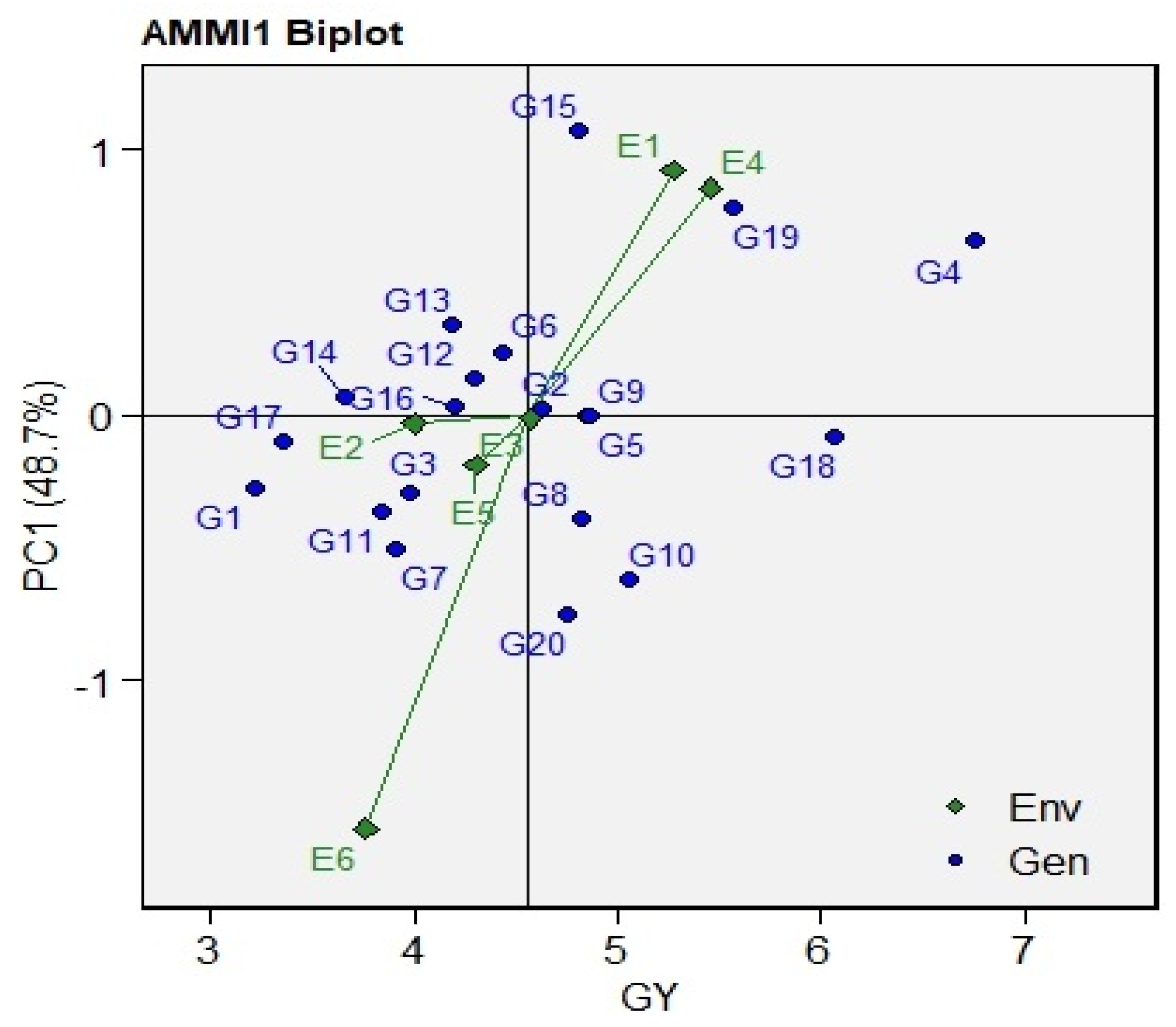
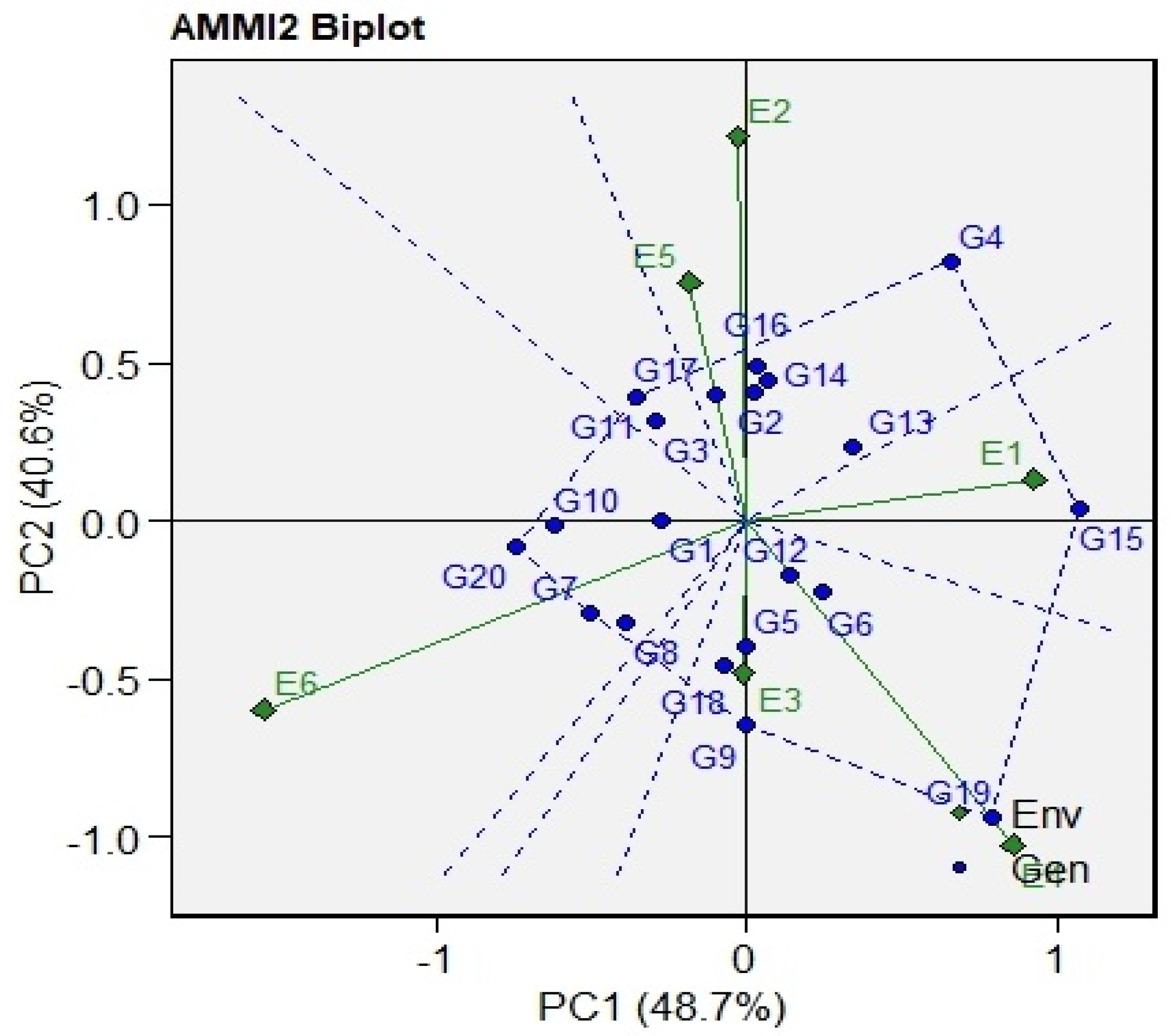
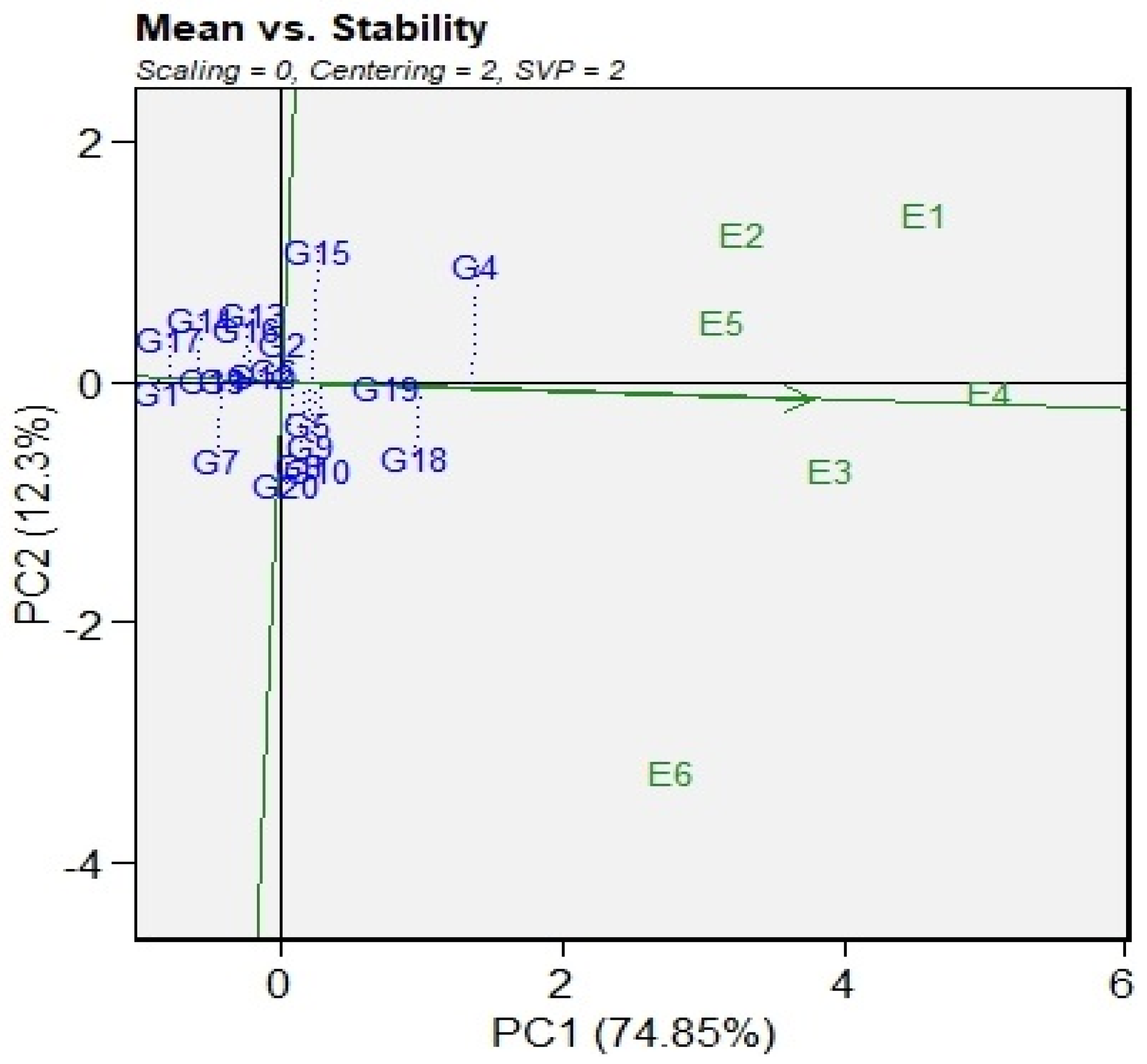
3.4. AMMI Biplot
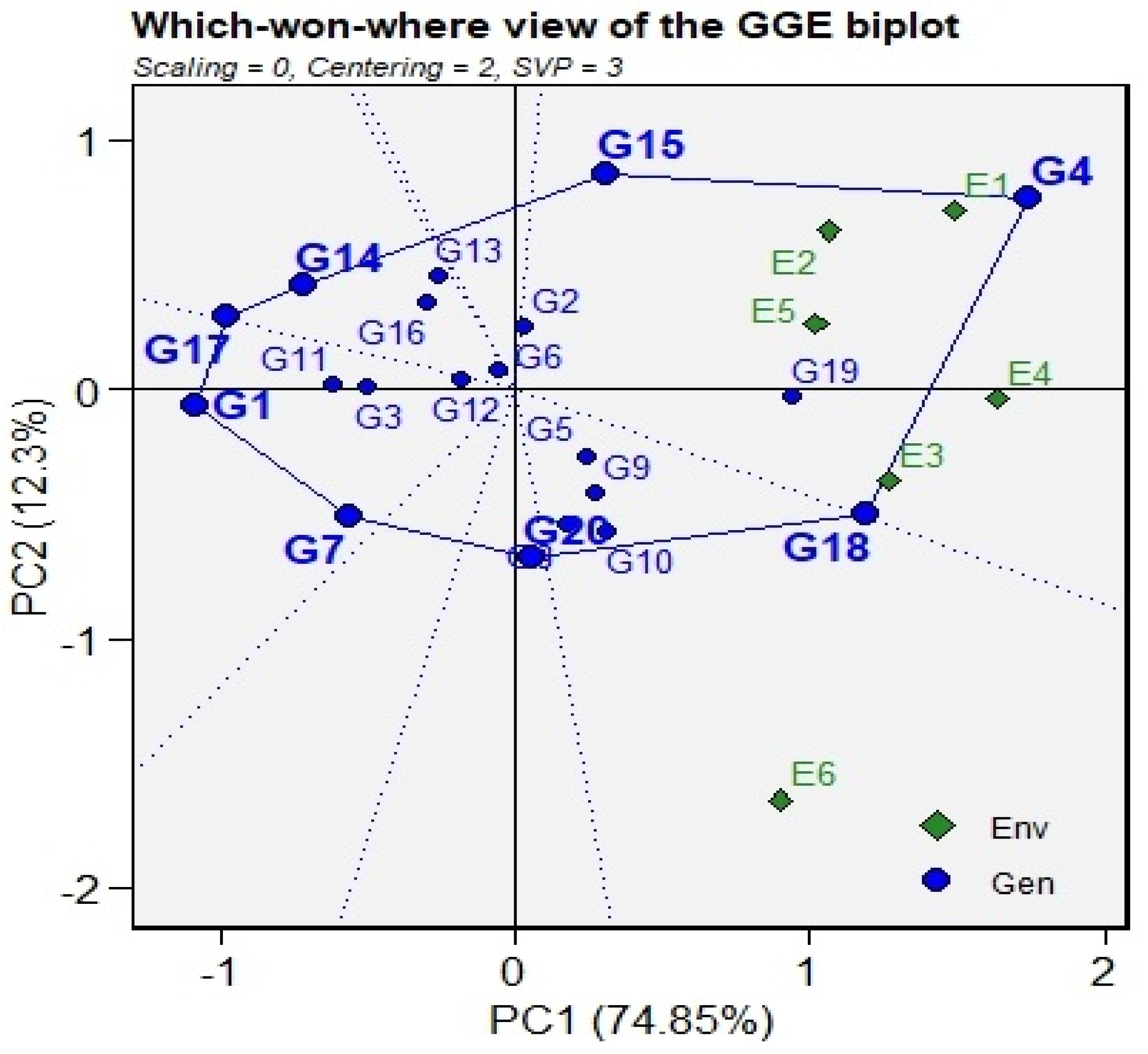
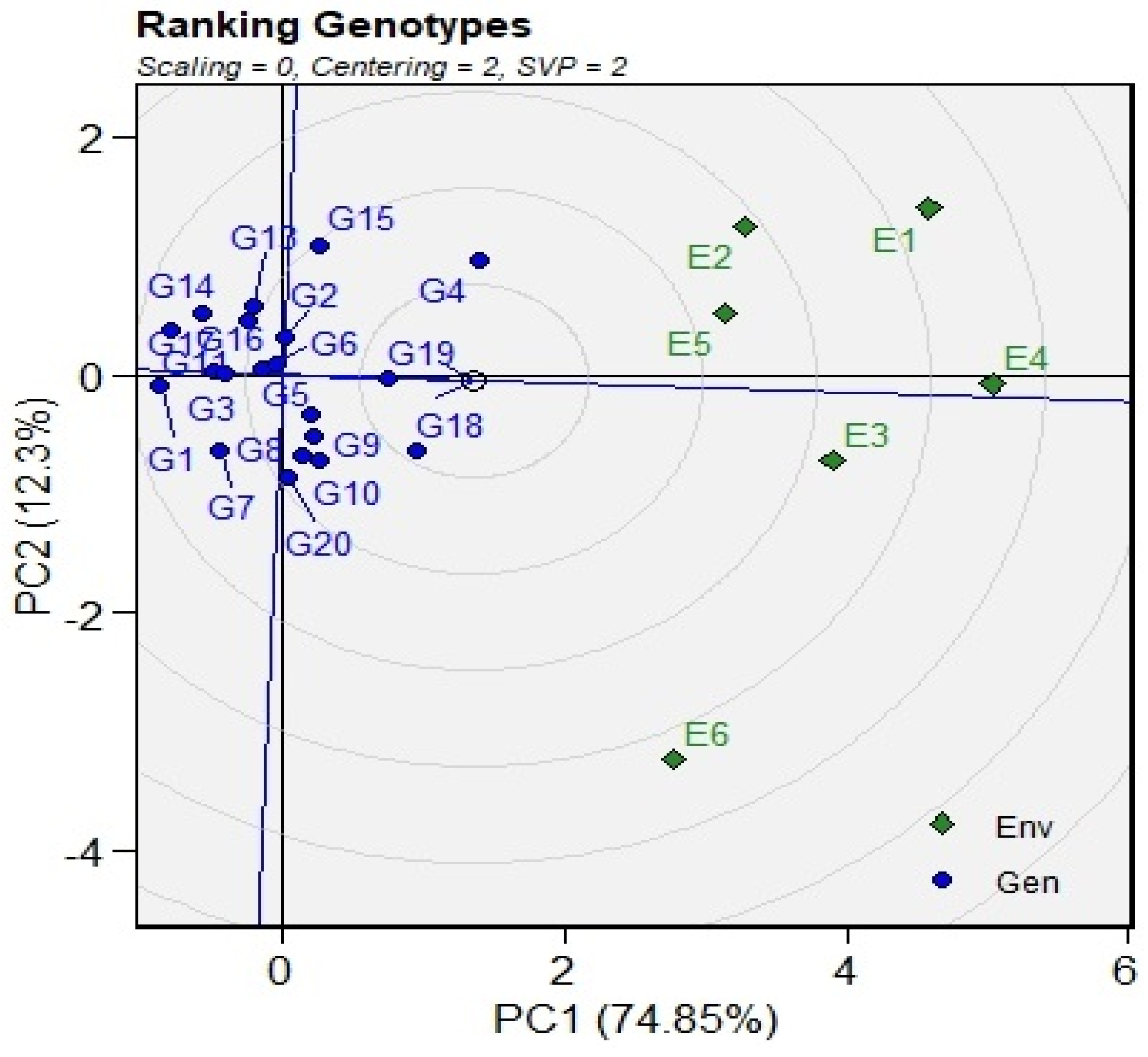
3.5. GGE Biplots
4. Discussion
5. Conclusions
Supplementary Materials
Author Contributions
Funding
Data Availability Statement
Acknowledgments
Conflicts of Interest
References
- Mondal, S.; Singh, R.P.; Mason, E.R.; Huerta-Espino, J.; Autrique, E.; Joshi, A.K. Grain yield, adaptation and progress in breeding for early-maturing and heat-tolerant wheat lines in South Asia. Field Crops Res. 2016, 192, 78–85. [Google Scholar] [CrossRef]
- Al-Ashkar, I.; Alotaibi, M.; Refay, Y.; Ghazy, A.; Zakri, A.; Al-Doss, A. Selection criteria for high-yielding and early-flowering bread wheat hybrids under heat stress. PLoS ONE 2020, 15, e0236351. [Google Scholar] [CrossRef]
- Abu-Zaitoun, S.Y.; Chandrasekhar, K.; Assili, S.; Shtaya, M.J.; Jamous, R.M.; Mallah, O.B.; Nashef, K.; Sela, H.; Distelfeld, A.; Alhajaj, N. Unlocking the genetic diversity within a Middle-East panel of durum wheat landraces for adaptation to semi-arid climate. Agronomy 2018, 8, 233. [Google Scholar] [CrossRef]
- Nie, Y.; Ji, W.; Ma, S. Assessment of heterosis based on genetic distance estimated using SNP in common wheat. Agronomy 2019, 9, 66. [Google Scholar] [CrossRef]
- Jabeen, M.; Gabriel, H.F.; Ahmed, M.; Mahboob, M.A.; Iqbal, J. Studying impact of climate change on wheat yield by using DSSAT and GIS: A case study of Pothwar region. In Quantification of Climate Variability, Adaptation and Mitigation for Agricultural Sustainability; Springer: Berlin/Heidelberg, Germany, 2017; pp. 387–411. [Google Scholar]
- Pachauri, R.K.; Allen, M.R.; Barros, V.R.; Broome, J.; Cramer, W.; Christ, R.; Church, J.A.; Clarke, L.; Dahe, Q.; Dasgupta, P. Climate Change 2014: Synthesis Report. Contribution of Working Groups I, II and III to the fifth Assessment Report of the Intergovernmental Panel on Climate Change; IPCC: Geneva, Switzerland, 2014. [Google Scholar]
- Bita, C.E.; Gerats, T. Plant tolerance to high temperature in a changing environment: Scientific fundamentals and production of heat stress-tolerant crops. Front. Plant Sci. 2013, 4, 273. [Google Scholar] [CrossRef]
- Zhao, C.; Liu, B.; Piao, S.; Wang, X.; Lobell, D.B.; Huang, Y.; Huang, M.; Yao, Y.; Bassu, S.; Ciais, P.; et al. Temperature increase reduces global yields of major crops in four independent estimates. Proc. Natl. Acad. Sci. USA 2017, 114, 9326–9331. [Google Scholar] [CrossRef]
- Qaseem, M.F.; Qureshi, R.; Muqaddasi, Q.H.; Shaheen, H.; Kousar, R.; Roder, M.S. Genome-wide association mapping in bread wheat subjected to independent and combined high temperature and drought stress. PLoS ONE 2018, 13, e0199121. [Google Scholar] [CrossRef]
- Hamidou, F.; Halilou, O.; Vadez, V.; Science, C. Assessment of groundnut under combined heat and drought stress. J. Agron. 2013, 199, 1–11. [Google Scholar] [CrossRef]
- Pradhan, G.P.; Prasad, P.V.V.; Fritz, A.K.; Kirkham, M.B.; Gill, B.S. Effects of drought and high temperature stress on synthetic hexaploid wheat. Funct. Plant Biol. 2012, 39, 190–198. [Google Scholar] [CrossRef]
- Awasthi, R.; Kaushal, N.; Vadez, V.; Turner, N.C.; Berger, J.; Siddique, K.H.M.; Nayyar, H. Individual and combined effects of transient drought and heat stress on carbon assimilation and seed filling in chickpea. Funct. Plant Biol. 2014, 41, 1148–1167. [Google Scholar] [CrossRef] [Green Version]
- Al-Ashkar, I.; Alderfasi, A.; Ben Romdhane, W.; Seleiman, M.F.; El-Said, R.A.; Al-Doss, A. Morphological and Genetic Diversity within Salt Tolerance Detection in Eighteen Wheat Genotypes. Plants 2020, 9, 287. [Google Scholar] [CrossRef]
- Evans, R.; Skaggs, R.; Sneed, R. Stress day index models to predict corn and soybean relative yield under high water table conditions. Trans. ASAE 1991, 34, 1997–2005. [Google Scholar] [CrossRef]
- Al-Ashkar, I.; Alderfasi, A.; El-Hendawy, S.; Al-Suhaibani, N.; El-Kafafi, S.; Seleiman, M.F. Detecting salt tolerance in doubled haploid wheat lines. Agronomy 2019, 9, 211. [Google Scholar] [CrossRef]
- Al-Ashkar, I.; Ibrahim, A.; Ghazy, A.; Attia, K.; Al-Ghamdi, A.A.; Al-Dosary, M.A. Assessing the correlations and selection criteria between different traits in wheat salt-tolerant genotypes. Saudi J. Biol. Sci. 2021, 28, 5414–5427. [Google Scholar] [CrossRef]
- Olivoto, T.; Lúcio, A.D.; da Silva, J.A.; Marchioro, V.S.; de Souza, V.Q.; Jost, E. Mean performance and stability in multi-environment trials I: Combining features of AMMI and BLUP techniques. Agron. J. 2019, 111, 2949–2960. [Google Scholar] [CrossRef]
- Singamsetti, A.; Shahi, J.; Zaidi, P.; Seetharam, K.; Vinayan, M.; Kumar, M.; Singla, S.; Shikha, K.; Madankar, K. Genotype × environment interaction and selection of maize (Zea mays L.) hybrids across moisture regimes. Field Crops Res. 2021, 270, 108224. [Google Scholar] [CrossRef]
- Kenga, R. Combining Ability Estimates and Heterosis in Selected Tropical Sorghum (Sorghum bicolor (L.) Moench); Department of Plant Science, Faculty of Agriculture, Ahmadu Bello University: Zaria, Nigeria, 2001; p. 186. [Google Scholar]
- Badu-Apraku, B.; Akinwale, R.; Menkir, A.; Obeng-Antwi, K.; Osuman, A.; Coulibaly, N.; Onyibe, J.; Yallou, G.; Abdullai, M.; Didjera, A. Use of GGE biplot for targeting early maturing maize cultivars to mega-environments in West Africa. Afr. Crop Sci. J. 2011, 19, 79–96. [Google Scholar] [CrossRef]
- Zobel, R.W.; Wright, M.J.; Gauch, H.G. Statistical-Analysis of a Yield Trial. Agron. J. 1988, 80, 388–393. [Google Scholar] [CrossRef]
- Knežević, D.; Zečević, V.; Đukić, N.; Dodig, D. Genetic and phenotypic variability of grain mass per spike of winter wheat genotypes (Triticum aestivum L.). Kragujev. J. Sci. 2008, 30, 131–136. [Google Scholar]
- Popović, V.; Ljubičić, N.; Kostić, M.; Radulović, M.; Blagojević, D.; Ugrenović, V.; Popović, D.; Ivošević, B. Genotype × Environment Interaction for Wheat Yield Traits Suitable for Selection in Different Seed Priming Conditions. Plants 2020, 9, 1804. [Google Scholar] [CrossRef]
- Mansour, E.; Moustafa, E.S.A.; Desoky, E.M.; Ali, M.M.A.; Yasin, M.A.T.; Attia, A.; Alsuhaibani, N.; Tahir, M.U.; El-Hendawy, S. Multidimensional Evaluation for Detecting Salt Tolerance of Bread Wheat Genotypes Under Actual Saline Field Growing Conditions. Plants 2020, 9, 1324. [Google Scholar] [CrossRef]
- Liersch, A.; Bocianowski, J.; Nowosad, K.; Mikołajczyk, K.; Spasibionek, S.; Wielebski, F.; Matuszczak, M.; Szała, L.; Cegielska-Taras, T.; Sosnowska, K.; et al. Effect of Genotype × Environment Interaction for Seed Traits in Winter Oilseed Rape (Brassica napus L.). Agriculture 2020, 10, 607. [Google Scholar] [CrossRef]
- Kendal, E. Comparing durum wheat cultivars by genotype× yield× trait and genotype× trait biplot method. Chil. J. Agric. Res. 2019, 79, 512–522. [Google Scholar] [CrossRef]
- Yan, W.; Fregeau-Reid, J. Genotype by Yield*Trait (GYT) Biplot: A Novel Approach for Genotype Selection based on Multiple Traits. Sci. Rep. 2018, 8, 8242. [Google Scholar] [CrossRef]
- Aprile, A.; Havlickova, L.; Panna, R.; Mare, C.; Borrelli, G.M.; Marone, D.; Perrotta, C.; Rampino, P.; De Bellis, L.; Curn, V.; et al. Different stress responsive strategies to drought and heat in two durum wheat cultivars with contrasting water use efficiency. BMC Genom. 2013, 14, 821. [Google Scholar] [CrossRef]
- Janzen, D.H.; Hallwachs, W. DNA barcoding the Lepidoptera inventory of a large complex tropical conserved wildland, Area de Conservacion Guanacaste, northwestern Costa Rica. Genome 2016, 59, 641–660. [Google Scholar] [CrossRef]
- El-Hennawy, M.A.; Abdalla, A.F.; Shafey, S.A.; Al-Ashkar, I.M. Production of doubled haploid wheat lines (Triticum aestivum L.) using anther culture technique. Ann. Agric. Sci. 2011, 56, 63–72. [Google Scholar] [CrossRef]
- Steel, R.G.D.; Torrie, J.H. Principles and Procedures of Statistics, a Biometrical Approach; McGraw-Hill Kogakusha, Ltd.: Irvine, CA, USA, 1980. [Google Scholar]
- Al-Ashkar, I.; Al-Suhaibani, N.; Abdella, K.; Sallam, M.; Alotaibi, M.; Seleiman, M.F. Combining Genetic and Multidimensional Analyses to Identify Interpretive Traits Related to Water Shortage Tolerance as an Indirect Selection Tool for Detecting Genotypes of Drought Tolerance in Wheat Breeding. Plants 2021, 10, 931. [Google Scholar] [CrossRef]
- Aebi, H.J.M. Catalase in vitro. Methods Enzymol. 1984, 105, 121–126. [Google Scholar]
- Chance, B.; Maehly, A. Preparation and assays of enzymes. Methods Enzymol. 1955, 2, 773–775. [Google Scholar]
- Duckworth, H.W.; Coleman, J.E. Physicochemical and kinetic properties of mushroom tyrosinase. J. Biol. Chem. 1970, 245, 1613–1625. [Google Scholar] [CrossRef]
- Shapiro, S.S.; Wilk, M.B. An Analysis of Variance Test for Normality (Complete Samples). Biometrika 1965, 52, 591–611. [Google Scholar] [CrossRef]
- Snedecor, G.; Cochran, W. Statistical Methods; Iowa State University Press: Ames, IA, USA, 1989. [Google Scholar]
- Vargas, M.; Crossa, J. The AMMI Analysis and Graphing the Biplot; Biometrics Statistics Unit; CIMMYT: Texcoco, Mexico, 2000. [Google Scholar]
- Purchase, J.L.; Hatting, H.; Van Deventer, C.S. Genotype × environment interaction of winter wheat (Triticum aestivum L.) in South Africa: II. Stability analysis of yield performance. S. Afr. J. Plant 2000, 17, 101–107. [Google Scholar] [CrossRef]
- Yan, W.; Hunt, L.A.; Sheng, Q.; Szlavnics, Z. Cultivar evaluation and mega-environment investigation based on the GGE biplot. Crop Sci. 2000, 40, 597–605. [Google Scholar] [CrossRef]
- Yan, W.; Tinker, N.A. Biplot analysis of multi-environment trial data: Principles and applications. Can. J. Plant Sci. 2006, 86, 623–645. [Google Scholar] [CrossRef]
- Crossa, J.; Cornelius, P.L.; Yan, W.J.C.S. Biplots of linear-bilinear models for studying crossover genotype× environment interaction. Crop Sci. 2002, 42, 619–633. [Google Scholar] [CrossRef]
- Yan, W. GGEbiplot—A Windows application for graphical analysis of multienvironment trial data and other types of two-way data. Agron. J. 2001, 93, 1111–1118. [Google Scholar] [CrossRef]
- Olivoto, T.; Lúcio, A.D. metan: An R package for multi-environment trial analysis. Methods Ecol. 2020, 11, 783–789. [Google Scholar] [CrossRef]
- Gollob, H.F. A statistical model which combines features of factor analytic and analysis of variance techniques. Psychometrik 1968, 33, 73–115. [Google Scholar] [CrossRef]
- Derera, J.; Tongoona, P.; Vivek, B.S.; Laing, M.D. Gene action controlling grain yield and secondary traits in southern African maize hybrids under drought and non-drought environments. Euphytica 2008, 162, 411–422. [Google Scholar] [CrossRef]
- Abakemal, D.; Shimelis, H.; Derera, J. Genotype-by-environment interaction and yield stability of quality protein maize hybrids developed from tropical-highland adapted inbred lines. Euphytica 2016, 209, 757–769. [Google Scholar] [CrossRef]
- Mebratu, A.; Wegary, D.; Mohammed, W.; Teklewold, A.; Tarekegne, A. Genotype × Environment Interaction of Quality Protein Maize Hybrids under Contrasting Management Conditions in Eastern and Southern Africa. Crop Sci. 2019, 59, 1576–1589. [Google Scholar] [CrossRef]
- Mason, R.E.; Singh, R.P. Considerations when deploying canopy temperature to select high yielding wheat breeding lines under drought and heat stress. Agronomy 2014, 4, 191–201. [Google Scholar] [CrossRef] [Green Version]
- Sah, R.P.; Chakraborty, M.; Prasad, K.; Pandit, M.; Tudu, V.K.; Chakravarty, M.K.; Narayan, S.C.; Rana, M.; Moharana, D. Impact of water deficit stress in maize: Phenology and yield components. Sci. Rep. 2020, 10, 2944. [Google Scholar] [CrossRef] [PubMed]
- Abdolshahi, R.; Nazari, M.; Safarian, A.; Sadathossini, T.S.; Salarpour, M.; Amiri, H. Integrated selection criteria for drought tolerance in wheat (Triticum aestivum L.) breeding programs using discriminant analysis. Field Crops Res. 2015, 174, 20–29. [Google Scholar] [CrossRef]
- El-Hendawy, S.; Al-Suhaibani, N.; Al-Ashkar, I.; Alotaibi, M.; Tahir, M.U.; Solieman, T.; Hassan, W.M. Combining Genetic Analysis and Multivariate Modeling to Evaluate Spectral Reflectance Indices as Indirect Selection Tools in Wheat Breeding under Water Deficit Stress Conditions. Remote Sens. 2020, 12, 1480. [Google Scholar] [CrossRef]
- Ebdon, J.; Gauch, H., Jr. Additive main effect and multiplicative interaction analysis of national turfgrass performance trials: I. Interpretation of genotype× environment interaction. Crop Sci. 2002, 42, 489–496. [Google Scholar] [CrossRef]
- Asfaw, A.; Alemayehu, F.; Gurum, F.; Atnaf, M. AMMI and SREG GGE biplot analysis for matching varieties onto soybean production environments in Ethiopia. Sci. Res. Essays 2009, 4, 1322–1330. [Google Scholar]
- Lin, C.-S.; Binns, M.R. A superiority measure of cultivar performance for cultivar× location data. Can. J. Plant Sci. 1988, 68, 193–198. [Google Scholar] [CrossRef]
- Kamidi, R.E. Relative stability, performance, and superiority of crop genotypes across environments. J. Agric. Biol. Environ. Stat. 2001, 6, 449–460. [Google Scholar] [CrossRef]
- Meng, T.Y.; Zhang, X.B.; Ge, J.L.; Chen, X.; Yang, Y.L.; Zhu, G.L.; Chen, Y.L.; Zhou, G.S.; Wei, H.H.; Dai, Q.G. Agronomic and physiological traits facilitating better yield performance of japonica/indica hybrids in saline fields. Field Crops Res. 2021, 271, 108255. [Google Scholar] [CrossRef]
- Elbasyoni, I.S. Performance and Stability of Commercial Wheat Cultivars under Terminal Heat Stress. Agronomy 2018, 8, 37. [Google Scholar] [CrossRef]
- Mafouasson, H.N.A.; Gracen, V.; Yeboah, M.A.; Ntsomboh-Ntsefong, G.; Tandzi, L.N.; Mutengwa, C.S. Genotype-by-Environment Interaction and Yield Stability of Maize Single Cross Hybrids Developed from Tropical Inbred Lines. Agronomy 2018, 8, 62. [Google Scholar] [CrossRef]
- Gauch Jr, H.G.; Zobel, R.W. Identifying mega-environments and targeting genotypes. Crop Sci. 1997, 37, 311–326. [Google Scholar] [CrossRef]
- Badu-Apraku, B.; Oyekunle, M.; Obeng-Antwi, K.; Osuman, A.; Ado, S.; Coulibay, N.; Yallou, C.; Abdulai, M.; Boakyewaa, G.; Didjeira, A. Performance of extra-early maize cultivars based on GGE biplot and AMMI analysis. J. Agric. Sci. 2012, 150, 473–483. [Google Scholar] [CrossRef]
- Yan, W.; Tinker, N.A. An integrated biplot analysis system for displaying, interpreting, and exploring genotype× environment interaction. Crop Sci. 2005, 45, 1004–1016. [Google Scholar] [CrossRef]
- Yan, W.; Rajcan, I. Biplot Analysis of Test Sites and Trait Relations of Soybean in Ontario. Crop Sci. 2002, 42, 11–20. [Google Scholar] [CrossRef]


| Parameters | Precipitation (mm) | Temperature (°C) | Relative Humidity (%) | ||||||||
|---|---|---|---|---|---|---|---|---|---|---|---|
| Months | Maximum | Minimum | Average | ||||||||
| S1 | S2 | S1 | S2 | S1 | S2 | S1 | S2 | S1 | S2 | ||
| November | 0.31 | 0.27 | 35.37 | 34.82 | 5.05 | 5.84 | 20.21 | 20.33 | 41.69 | 41.21 | |
| December | 0.02 | 0.10 | 27.40 | 27.46 | 4.01 | 4.95 | 15.71 | 16.21 | 45.31 | 44.36 | |
| January | 0.10 | 0.05 | 29.34 | 28.65 | 1.23 | 2.01 | 15.29 | 15.33 | 40.19 | 40.68 | |
| February | 0.00 | 0.00 | 33.79 | 32.43 | 1.21 | 2.08 | 17.50 | 17.26 | 28.44 | 29.26 | |
| March | 0.00 | 0.00 | 35.80 | 36.19 | 6.98 | 7.01 | 21.39 | 21.60 | 25.69 | 26.02 | |
| April | 0.98 | 1.02 | 39.91 | 38.63 | 14.13 | 15.11 | 27.02 | 26.87 | 31.50 | 30.24 | |
| May | 0.01 | 0.00 | 42.91 | 41.77 | 19.21 | 19.94 | 31.06 | 30.86 | 17.69 | 17.05 | |
| S.O.V | Environment (E) | Genotypes (G) | GEI | Error | |||
|---|---|---|---|---|---|---|---|
| df | 5 | 19 | 95 | 238 | |||
| Traits | Mean Squares | % (G + E + GEI) | Mean Squares | % (G + E + GEI) | Mean Squares | % (G + E + GEI) | Mean Squares |
| CT | 94.606 *** | 75.291 | 3.441 *** | 10.406 | 0.939 *** | 14.201 | 0.078 |
| LWC | 519.504 *** | 42.010 | 84.017 *** | 25.818 | 20.426 *** | 31.383 | 8.156 |
| RWC | 1030.553 *** | 39.732 | 225.212 *** | 32.994 | 35.812 *** | 26.233 | 15.893 |
| Pn | 24.459 *** | 12.139 | 40.972 *** | 77.274 | 1.109 *** | 10.462 | 0.689 |
| Gs | 0.037 *** | 39.001 | 0.009 *** | 35.554 | 0.001 *** | 25.307 | 0.000 |
| Ci | 54,819.43 *** | 53.337 | 8120.35 *** | 30.023 | 793.908 *** | 14.676 | 230.166 |
| E | 8.444 *** | 47.235 | 1.333 *** | 28.326 | 0.229 *** | 24.386 | 0.031 |
| POD | 0.000 *** | 0.016 | 0.009 *** | 66.068 | 0.001 *** | 33.912 | 0.000 |
| PPO | 0.001 *** | 16.329 | 0.001 *** | 48.615 | 0.000 *** | 35.043 | 0.000 |
| CAT | 0.000 *** | 8.547 | 0.001 *** | 63.625 | 0.000 *** | 27.819 | 0.000 |
| GLN | 3.093 *** | 20.737 | 1.855 *** | 47.253 | 0.248 *** | 31.529 | 0.064 |
| FLA | 199.631 *** | 12.531 | 327.214 *** | 78.048 | 7.824 *** | 9.331 | 1.169 |
| GLA | 8783.515 *** | 30.323 | 4026.602 *** | 52.824 | 253.939 *** | 16.657 | 29.207 |
| LAI | 87.868 *** | 56.499 | 9.802 *** | 23.949 | 1.599 *** | 19.536 | 0.030 |
| DH | 357.610 *** | 30.122 | 206.951 *** | 67.028 | 1.662 * | 2.705 | 1.204 |
| MD | 2412.849 *** | 72.206 | 184.713 *** | 21.005 | 11.877 *** | 6.753 | 1.613 |
| GFD | 976.502 *** | 66.842 | 61.481 *** | 15.992 | 13.144 *** | 17.095 | 2.200 |
| NS | 468,877.09 *** | 54.842 | 48,130.84 *** | 21.392 | 10,648.73 *** | 23.665 | 737.254 |
| PH | 1064.972 *** | 23.920 | 726.276 *** | 61.988 | 31.977 *** | 13.646 | 9.845 |
| SL | 46.666 *** | 37.542 | 11.201 *** | 34.241 | 1.835 *** | 28.054 | 0.210 |
| NSS | 100.678 *** | 33.624 | 32.430 *** | 41.157 | 3.871 *** | 24.565 | 0.405 |
| NGS | 635.356 *** | 23.742 | 405.946 *** | 57.643 | 26.121 *** | 18.546 | 3.933 |
| TKW | 1627.585 *** | 44.743 | 473.567 *** | 49.470 | 10.918 *** | 5.702 | 3.539 |
| GY | 28.119 *** | 28.053 | 13.660 *** | 51.786 | 1.057 *** | 20.036 | 0.062 |
| Environments | No. of Variables | Variables | Variable IN/OUT | R2 | R2 Com. | Pr > F |
|---|---|---|---|---|---|---|
| E1 | 1 | TKW | TKW | 0.584 | 0.584 | <0.0001 |
| 2 | GLA/TKW | GLA | 0.265 | 0.850 | <0.0001 | |
| E2 | 1 | FLA | FLA | 0.466 | 0.466 | <0.0001 |
| 2 | FLA/POD | POD | 0.433 | 0.899 | <0.0001 | |
| E3 | 1 | FLA | FLA | 0.506 | 0.506 | <0.0001 |
| 2 | PH/FLA | PH | 0.199 | 0.705 | <0.0001 | |
| 3 | PH/FLA/TKW | TKW | 0.149 | 0.853 | <0.0001 | |
| 4 | PH/FLA/TKW/Pn | Pn | 0.034 | 0.888 | 0.000 | |
| E4 | 1 | GLA | GLA | 0.540 | 0.540 | <0.0001 |
| 2 | GLA/TKW | TKW | 0.301 | 0.841 | <0.0001 | |
| E5 | 1 | FLA | FLA | 0.585 | 0.585 | <0.0001 |
| 2 | FLA/POD | POD | 0.279 | 0.863 | <0.0001 | |
| E6 | 1 | POD | POD | 0.607 | 0.607 | <0.0001 |
| 2 | FLA/POD | FLA | 0.313 | 0.920 | <0.0001 | |
| pooled data (E3 and E6) | 1 | FLA | FLA | 0.462 | 0.462 | 0.001 |
| 2 | FLA/Pn | Pn | 0.272 | 0.734 | <0.0001 | |
| 3 | FLA/Pn/POD | POD | 0.225 | 0.859 | <0.0001 | |
| 4 | PH/FLA/Pn/POD | PH | 0.014 | 0.873 | <0.0001 | |
| pooled data (E2 and E5) | 1 | FLA | FLA | 0.515 | 0.515 | <0.0001 |
| 2 | FLA/POD | POD | 0.369 | 0.884 | <0.0001 | |
| pooled data (E1 and E4) | 1 | GLA | GLA | 0.506 | 0.506 | <0.0001 |
| 2 | GLA/TKW | TKW | 0.338 | 0.844 | <0.0001 | |
| pooled data (S1) | 1 | FLA | FLA | 0.427 | 0.427 | 0.000 |
| 2 | GFD/FLA | GFD | 0.144 | 0.571 | <0.0001 | |
| 3 | GFD/FLA/GLA | GLA | 0.111 | 0.682 | <0.0001 | |
| 4 | GFD/FLA/GLA/LWC | LWC | 0.110 | 0.792 | 0.005 | |
| 5 | GFD/FLA/GLA/LWC/TKW | TKW | 0.018 | 0.810 | 0.002 | |
| 6 | DH/GFD/FLA/GLA/LWC/TKW | DH | 0.008 | 0.818 | 0.000 | |
| pooled data (S2) | 1 | FLA | FLA | 0.309 | 0.309 | <0.0001 |
| 2 | FLA/POD | POD | 0.228 | 0.537 | <0.0001 | |
| 3 | GFD/FLA/POD | GFD | 0.143 | 0.680 | <0.0001 | |
| 4 | GFD/PH/FLA/POD | PH | 0.116 | 0.796 | 0.002 | |
| 5 | GFD/PH/FLA/Pn/POD | Pn | 0.039 | 0.835 | <0.0001 | |
| 6 | GFD/PH/FLA/TKW/Pn/POD | TKW | 0.029 | 0.864 | <0.0001 | |
| All pooled data (S1 and S2) | 1 | FLA | FLA | 0.306 | 0.306 | <0.0001 |
| 2 | GFD/FLA | GFD | 0.201 | 0.507 | <0.0001 | |
| 3 | GFD/PH/FLA | PH | 0.121 | 0.628 | 0.019 | |
| 4 | GFD/PH/FLA/POD | POD | 0.106 | 0.734 | <0.0001 | |
| 5 | GFD/PH/FLA/TKW/POD | TKW | 0.035 | 0.769 | 0.002 | |
| 6 | DH/GFD/PH/FLA/TKW/POD | DH | 0.029 | 0.798 | <0.0001 | |
| 7 | DH/GFD/PH/FLA/LWC/TKW/POD | LWC | 0.023 | 0.821 | <0.0001 |
| Environments | Equation |
|---|---|
| E1 | GY = −2.636 + 0.034 × GLA + 0.102 × TKW |
| E2 | GY = −1.886 + 0.035 × GLA + 0.085 × TKW |
| E3 | GY = 1.504 + 0.1394 × FLA + 12.3144 × POD |
| E4 | GY = 1.575 + 0.140 × FLA + 12.244 × POD |
| E5 | GY = −1.420 + 0.380 × PH + 0.131 × FLA − 0.040 × TKW + 0.1891 × Pn |
| E6 | GY = 0.810 + 0.124 × FLA + 49.752 × POD |
| pooled data (E3 and E6) | GY = −2.275 + 0.034 × GLA + 0.094 × TKW |
| pooled data (E2 and E5) | GY = 1.490 + 0.143 × FLA + 12.094 × POD |
| pooled data (E1 and E4) | GY = −1.698 + 0.017 × PH + 0.128 × FLA + 0.234 × Pn − 18.686 × POD |
| pooled data (S1) | GY = −3.110 + 0.036 × DH + 0.080 × GFD + 0.150 × FLA + 0.006 × GLA − 0.031 × LWC + 0.028 × TKW |
| pooled data (S2) | GY = −2.431 + 0.024 × GFD + 0.015 × PH + 0.146 × FLA + 0.022 × TKW + 0.074 × Pn + 9.121 × POD |
| All pooled data (S1 and S2) | GY = −3.265 + 0.034 × DH + 0.031 × GFD + 0.009 × PH + 0.145 × FLA − 0.013 × LWC + 0.028 × TKW + 6.115 × POD |
| Source | df | SS | MS | F-Value | Total Variation Explained (%) |
|---|---|---|---|---|---|
| Total | 359 | 515.90 | 1.437 | ||
| Treatments | 119 | 500.60 | 4.206 | 67.18 *** | 97.034 |
| Genotypes | 19 | 259.50 | 13.660 | 218.17 *** | 50.300 |
| Environments | 5 | 140.60 | 28.119 | 310.94 *** | 27.253 |
| Block | 12 | 1.10 | 0.090 | 1.44 ns | 0.213 |
| Interactions | 95 | 100.40 | 1.057 | 16.88 *** | 19.461 |
| IPCA [1] | 23 | 48.70 | 2.117 | 33.8 *** | 48.706 |
| IPCA [2] | 21 | 41.00 | 1.952 | 31.18 *** | 40.637 |
| IPCA [3] | 19 | 6.30 | 0.334 | 5.33 *** | 6.275 |
| IPCA [4] | 17 | 4.30 | 0.255 | 4.07 *** | 4.283 |
| Residuals | 15 | 0.10 | 0.004 | 0.07 ns | 0.100 |
| Error | 228 | 14.30 | 0.063 |
| Genotypes | Gm | Score (A) | IPCAg [1] | Score [1] | IPCAg [2] | Score [2] | ASV | Score (B) | YSI (A + B) | Superiority | |||
|---|---|---|---|---|---|---|---|---|---|---|---|---|---|
| GY | Score | MT | Score | ||||||||||
| DHL12 (G1) | 3.232 | 20 | 0.275 | 10 | 0.014 | 3 | 11.583 | 3 | 23 | 2.273 | 20 | 0.771 | 12 |
| DHL02 (G2) | 4.660 | 10 | −0.036 | 3 | 0.407 | 13 | 13.658 | 5 | 15 | 0.908 | 9 | 0.706 | 10 |
| DHL25 (G3) | 4.005 | 15 | 0.283 | 11 | 0.330 | 10 | 15.765 | 8 | 23 | 1.460 | 15 | 0.983 | 19 |
| DHL07 (G4) | 5.997 | 2 | −0.683 | 17 | 0.798 | 19 | 26.302 | 19 | 21 | 0.040 | 1 | 0.362 | 1 |
| DHL26 (G5) | 4.869 | 6 | 0.015 | 1 | −0.395 | 11 | 11.215 | 2 | 8 | 0.819 | 5 | 0.637 | 5 |
| Gemmeiza-9 (G6) | 4.459 | 11 | −0.233 | 9 | −0.233 | 7 | 12.361 | 4 | 15 | 1.076 | 11 | 0.543 | 2 |
| DHL11 (G7) | 3.922 | 16 | 0.513 | 15 | −0.274 | 8 | 18.057 | 14 | 30 | 1.621 | 17 | 0.638 | 6 |
| KSU106 (G8) | 4.841 | 7 | 0.403 | 14 | −0.306 | 9 | 17.654 | 11 | 18 | 0.879 | 8 | 0.657 | 9 |
| Gemmeiza-12 (G9) | 4.885 | 5 | 0.020 | 2 | −0.644 | 18 | 18.280 | 15 | 20 | 0.849 | 7 | 1.007 | 20 |
| DHL01 (G10) | 5.087 | 4 | 0.620 | 16 | 0.006 | 2 | 17.304 | 10 | 14 | 0.728 | 4 | 0.945 | 18 |
| DHL14 (G11) | 3.870 | 17 | 0.348 | 13 | 0.408 | 14 | 19.932 | 17 | 34 | 1.592 | 16 | 0.804 | 14 |
| DHL29 (G12) | 4.318 | 12 | −0.133 | 8 | −0.176 | 5 | 10.460 | 1 | 13 | 1.183 | 12 | 0.543 | 3 |
| DHL15 (G13) | 4.213 | 14 | −0.345 | 12 | 0.223 | 6 | 14.489 | 7 | 21 | 1.245 | 14 | 0.548 | 4 |
| DHL06 (G14) | 3.684 | 18 | −0.081 | 5 | 0.446 | 15 | 16.226 | 9 | 27 | 1.734 | 18 | 0.877 | 16 |
| Misr1 (G15) | 4.83 | 8 | −1.073 | 20 | 0.004 | 1 | 21.211 | 18 | 26 | 0.832 | 6 | 0.901 | 17 |
| DHL05 (G16) | 4.23 | 13 | −0.046 | 4 | 0.489 | 17 | 17.774 | 12 | 25 | 1.227 | 13 | 0.808 | 15 |
| DHL23 (G17) | 3.37 | 19 | 0.090 | 6 | 0.405 | 12 | 13.988 | 6 | 25 | 2.082 | 19 | 0.789 | 13 |
| Sakha-93 (G18) | 6.04 | 1 | 0.092 | 7 | −0.452 | 16 | 17.973 | 13 | 14 | 0.252 | 2 | 0.641 | 7 |
| Pavone-76 (G19) | 5.49 | 3 | −0.758 | 19 | −0.964 | 20 | 28.417 | 20 | 23 | 0.541 | 3 | 0.653 | 8 |
| DHL08 (G20) | 4.79 | 9 | 0.728 | 18 | −0.087 | 4 | 19.600 | 16 | 25 | 0.940 | 10 | 0.713 | 11 |
Publisher’s Note: MDPI stays neutral with regard to jurisdictional claims in published maps and institutional affiliations. |
© 2022 by the authors. Licensee MDPI, Basel, Switzerland. This article is an open access article distributed under the terms and conditions of the Creative Commons Attribution (CC BY) license (https://creativecommons.org/licenses/by/4.0/).
Share and Cite
Al-Ashkar, I.; Sallam, M.; Al-Suhaibani, N.; Ibrahim, A.; Alsadon, A.; Al-Doss, A. Multiple Stresses of Wheat in the Detection of Traits and Genotypes of High-Performance and Stability for a Complex Interplay of Environment and Genotypes. Agronomy 2022, 12, 2252. https://doi.org/10.3390/agronomy12102252
Al-Ashkar I, Sallam M, Al-Suhaibani N, Ibrahim A, Alsadon A, Al-Doss A. Multiple Stresses of Wheat in the Detection of Traits and Genotypes of High-Performance and Stability for a Complex Interplay of Environment and Genotypes. Agronomy. 2022; 12(10):2252. https://doi.org/10.3390/agronomy12102252
Chicago/Turabian StyleAl-Ashkar, Ibrahim, Mohammed Sallam, Nasser Al-Suhaibani, Abdullah Ibrahim, Abdullah Alsadon, and Abdullah Al-Doss. 2022. "Multiple Stresses of Wheat in the Detection of Traits and Genotypes of High-Performance and Stability for a Complex Interplay of Environment and Genotypes" Agronomy 12, no. 10: 2252. https://doi.org/10.3390/agronomy12102252