Abstract
Valencian citriculture is oriented towards fresh production, which requires fruits with few seeds or seedless fruits. Consequently, parthenocarpic and self-incompatible varieties are mainly cultivated. However, some mandarin varieties, under favorable circumstances, induce seed formation in other mandarins by cross-pollination. This phenomenon depends on the germination capacity of the pollen of the pollinating variety, the number of ovules of the pollinated variety, the distance between them, and the abundance of pollinating insects. Previous studies in Instituto Valenciano de Investigaciones Agrarias (IVIA) have determined the ability to pollinate and be pollinated by all commercial varieties in Europe. Moreover, the Regional Government, Generalitat Valenciana, has georeferenced information on the cultivated varieties. We present two geostatistical models to estimate the risk of plots to be pollinated, depending on the varieties present in their environment, the number of plants, and their distance. Models are used to generate local and regional cross-pollination risk maps. Moreover, the robustness of these models to changes in the values assigned to their main parameters is assessed using different similarity calculations.
1. Introduction
Spain is the largest citrus producer in Europe and sixth in the world [1], with a production of 6,257,696,000 kg in 2019 [2]. Comunitat Valenciana is the major citrus-growing region at national level, both in terms of area, with 159,248 ha representing 53.7% of the national total in 2019, and in terms of production, with 3,067,517,000 kg representing 49% of the national production in the same year [2,3]. Valencian producers have a strong exporting vocation, mainly of products destined for fresh consumption and with high quality standards. According to the Food and Agriculture Organization of the United Nations (FAO), Spain is the world’s major citrus exporter [1]. In Spain, 43.8% of the 2019 production (2,743,791,000 kg) was destined to foreign markets [2].
Citrus orchards cover 29.1% of the agricultural land of the Valencian Community. The Valencian citriculture is mostly dedicated to the production of orange and mandarins (45.9% and 44.2% of the citrus production, respectively) for the fresh consumption market [3], where seedless fruits have much higher prices. For this reason, parthenocarpic and self-incompatible varieties, which prevent seed generation, have been traditionally cultivated. Some of newly introduced varieties, most of them obtained by hybridization processes, have the ability to pollinate already established orchards under favorable circumstances, thus inducing the formation of seeds. This phenomenon is known as cross-pollination. It depends, among other factors, on the germination capacity of the pollen grains of the pollinating variety; the number of ovules of the pollinated variety; the distance between plants; the presence of pollinating insects; the weather conditions before, during, and after blooming; the coincidence in time of both blooming seasons; the orientation of the rows; and the presence of hedges or barriers.
Wind pollination of commercial citrus is negligible as pollen is heavy and sticky [4]. Moreover, citrus produce nectar copiously that is secreted continuously for at least 48 h after the flower opening [5]. Citrus nectar is a major attractant for bees (Apis mellifera), which have evolved to optimize the cost of searching for food, in terms of time and energy. Their flight distance varies with weather conditions and the flowering of surrounding plants [6].
With the aim of making citrus farming compatible with beekeeping and with citrus flower honey production, Generalitat Valenciana traditionally establishes temporal measures to limit cross-pollination between citrus plantations. These include the limitation or prohibition of the settlement of beehives in the vicinity of crops in those areas and municipal districts where a high risk of cross-pollination during the flowering period may occur. Times and areas are currently estimated from the meteorological data recorded and weather forecast for next spring. Likewise, it regulates the use of phytosanitary products by farmers, so that only harmless products and practices are allowed and applied at times when bees do not forage [7].
In this context, it is imperative to design new tools to manage citrus cross-pollination risks impartially, using scientific knowledge and ground data. Contrary to citrus grown in Spain, pollination or cross-pollination may be beneficial for many species, thus considered an essential ecosystem service. However, they may also cause undesired effects for other crops, for instance, pollination of surrounding cultivated or wild species by genetically modified crops. Furthermore, sensible people suffer from allergies owing to the pollen of different plant species and it is important to forecast their level in the atmosphere. Being different applications, different approaches are found in the literature.
An example of the first applications (pollination as ecosystem service) can be found in [8], with further development in [9], where the objective is to understand the contributions of landscape elements to pollinator populations and to crop pollination.
On the other hand, Lipsius et al. [10] proposed Lagrangian approaches to model pollen dispersal from a genetically modified maize field. These models proved to be appropriate for the simulation of the cross-pollination rates, but performances differed between years.
Suano et al. [11] reported a methodical review of methods to predict atmospheric pollen level prediction, aimed at avoiding health burdens to the sensitive population.
At this point, we should remark the differences between risk and probability. Risk is the level of possibility that an action leads to an undesired outcome. Risks may even pay off and not lead to a loss but to a gain. On the other hand, probability is an estimation of how likely is it that an event will occur.
This work focuses on spatially representing cross-pollination risks that affect citrus orchards in Spanish conditions, because, once the orchards have been planted, it is highly expensive to replant them. Cross-pollination risks of an orchard derive from the variety that is planted, the amount of plan material, its location, and these same characteristics of the surrounding citrus orchards and the presence or absence of pollinators. However, the probability of pollination occurring depends on meteorological and climatic factors combined with the abundancy of pollinators and landscape configuration.
The geostatistical models developed in this work to estimate the distribution of the risk of cross-pollination in our territory were created taking advantage of current free online services capable of easy modelling and fast data analysis, without increasing the demand for local computing resources. One of them is Google Earth Engine. Our models were developed in close cooperation with the stakeholders in such a way that the results are visibly interpretable, and both the models and the results can be easily discussed and improved. Two models were built using the same base hypothesis, as defined in Section 2.2. One is developed at local scale, in which risks are calculated at individual orchard level, and another is aimed at representing a regional scale, by aggregating such individual risks into larger tiles to produce large scale maps. Their differences are described in Section 2.3.
As models must demonstrate their robustness, a complementary objective of this work is to analyze the sensitivity of the developed models to changes in the values of the main variables (those linked to the fundamental hypotheses). Robustness is examined for both models (Section 2.4) by analyzing similarities in terms of data or image correlation and, in the case of images, also in terms of structural similarity, via the structural similarity index measure (SSIM) described in [12]. Section 3 describes the obtained maps and the results of robustness analysis, while Section 4 discusses the novelties and implications of the work.
2. Materials and Methods
2.1. Data Sources and Pretreatment
Models are based on two data sources:
- An official database containing geo-referenced information of 219,239 citrus plots and the declaration of the citrus variety grown (hereinafter named REGEPA).
- Studies carried out by the IVIA for more than 25 years, assessing (a) the capacity of each commercial variety to induce seeds in the others and (b) their sensitivity to pollination by other citrus [13]. An example of how these data are represented is shown in Table 1.
 Table 1. Example of pollination data generated by IVIA for two common varieties.
A preliminary study of the REGEPA database revealed some incoherencies (i.e., duplicated geometries, null area geometries) in a negligible amount (0.5%) of the records. These incoherencies were filtered using open GIS software (QGIS [14] and MapShaper [15]), resulting in 218,203 valid records, which represents approximately 53% of current citrus orchards cultivated in Comunitat Valenciana.
Furthermore, synonyms were detected (records referring to the same variety but having the field ‘variety’ with different codes). Synonyms were resolved by changing the field ‘variety’ of these records to a single code.
2.2. Basis of Both Geostatistical Models
As noted earlier, two models were built, one representing local scales and another at representing regional scales. Both are based on the hypothesis that, for a particular citrus plot, the risk of its trees being pollinated depends on the following attributes of its own and surrounding citrus plots:
- Plant material (varieties) involved;
- Amount of susceptible plants;
- The ability of bees and other pollinating insects to fly from one plot to another.
Consequently, the following assumptions were made:
- Related to the plant material:
- (a)
- Related to the ability of bees and other pollinating insects to reach both plots Clementines and other varieties have self-incompatibility, their pollen does not induce seeds to themselves, as reported in [13].
- (b)
- Spring blooming of lemons is lower than that of oranges and mandarins, so their germinative power is divided by 2.
- (c)
- The capacity for a variety to pollinate (pol_ab) another variety is proportional to the following:pol_ab = germinative power (pollinator) ∗ viable ovules (pollinated)/100
- Related to the amount of plants:
- (d)
- The quantity of vegetation is proportional to the area of affected plots (the pollinator and the pollinated).
- Related to the ability of bees and other pollinating insects to reach both plots:
- (e)
- The ability of bees and other pollinating insects to pollinate decreases proportionally with distance until it becomes zero.
- (f)
- The maximum flight distance of bees (Mf) is 3000 m, a value consistent with [6].
The model is implemented as follows:
- Filter all of the sensible plots (plots having a variety that can be pollinated).
- For each of such plots:
- Find all the neighbouring plots in a 3000 m radius.The risk induced by each of these plots (rn) is calculated using the following equation:where pol_ab is the pollination ability of the neighbor plot (Equation (1)); f implements assumption (d), a proportionality factor related to plot surface (it is squared as it is the same for both orchards); a is the area of the sensible plot, a1 is the area of the neighbor plot, d is the distance between plots, and Mf is the maximum flight distance of bees.rn = pol_ab* f2 ∗ a* ai ∗ (1 − d/Mf)
- Calculate the risk score of a particular plot i (Ri), which is the sum of the risk induced from each of its neighboring plots.Ri = ∑ rn
2.3. Differences between the Local and Regional Model: Respective Map Generation
Once the risk score of each individual plot is calculated, the local model is constructed and directly represented as a vector layer in low scale maps. These maps are aimed at taking measures at the local level (municipality, cooperative, farmer or beekeeper association, large enterprises, and so on). Calculated risk scores of plots are directly represented in a linear scale from green (lower risks) to red (higher risks).
The regional model is aimed at locating the hot spots at the regional level. It requires the following further processing steps:
- Generate a squared 3 km × 3 km grid at the regional level.
- Sum risk scores of plots located under each of the grid elements and generate a pixel gray level of a raster layer, hereinafter referred as a raw image.
- Normalize gray levels by dividing them by the 95th percentile of the dynamic range. This percentile value was selected instead of the maximum gray level to avoid the effect of excessively large gray levels that would reduce the dynamic range of the normalized image. The resulting image is hereinafter referred as the normalized image.
Finally, in order to provide a smoother view of this layer, a moving average filter is applied to the raw image to generate the hereinafter called smoothed image. Risks are represented in the smoothed image using a palette from green (lower risks) to red (higher risks) in a stepped scale:
- (1)
- Values from the 0 to 20th percentile are represented as maximum green (hexadecimal value 00FF00h).
- (2)
- Values >20th percentile and <95th percentile are represented in a linear scale from maximum green to maximum red (hexadecimal value FF0000h).
- (3)
- Values higher than the 95th percentile are represented as maximum red.
2.4. Robustness Assessment
Robustness assessment assumed that both declared varieties of the plots and orchard surfaces are correct, as they are inspected by the regional government. Therefore, if we look at Equation (2), two variables influence the risk score of a plot: f, a proportionality factor related to plot surface, and Mf, the maximum flight distance of bees.
Subsequently, arbitrary different values for these variables were used to recalculate risks, which were then compared with the original reference values (f = 1/2.5 per ha and Mf, = 3000 m). Arbitrary values of f were determined by multiplying the reference value by 0.5, 0,82, 1.15, and 1.29, which represent 1/4, 2/3, 4/3, and 5/3 changes, respectively, in the effect of the amount of vegetation in Equation (2) (because f is squared) from the original model. Arbitrary values of Mf were 2000, 2500, 4000, and 5000 m, which represent 2/3, 2.5/3, 4/3, and 5/3 changes, respectively, in the effect of the amount of vegetation in Equation (2) from the original model.
In the case of vector and raster representations, comparisons were made by calculating the Pearson’s correlation coefficient (r) and the root mean squared error (RMSE) between the reference and recalculated scores or gray level values.
However, in raster representations, these metrics use absolute or relative differences of pixel gray level values that do not consider differences in the structural information present in the images, which are of relevant importance for human visual perception. For this reason, we used the structural similarity index (SSIM) described in [12]. This index is the combination of three functions that independently compare the luminance (l(x,y)), contrast (c(x,y)), and correlation (s(x,y)) of both images:
SSIM(x,y) = [l(x,y)]α · [c(x,y)]β · [s(x,y)]γ
The index was implemented assuming α = β = γ = 1 and coefficients C1 = C2 = C3 = 0 (not shown in Equation (4)), because sums of squared means and sums of squared standard deviations are far from being 0 in our images. As a consequence, we used a particular case of SSIM implementation that corresponds to the universal quality index described in [16]. Values of SSIM, l, c, and s were calculated for each raster comparison.
Robustness assessment of the local model was performed by calculating r and RMSE, on raw and normalized (divided by the maximum value) risk scores. In order to reduce the effect of zero risk orchard scores in the results, only orchards planted with sensitive varieties were considered in this analysis.
Robustness assessment of the regional model was performed by calculating RMSE, SSIM, l, c, and s on normalized risk gray level images, masking pixels outside the citrus growing area in order to avoid excessive 0 gray level pixels that will hide differences in these parameters.
3. Results
3.1. Graphical Representation of Models
Figure 1 shows the calculated risk scores of individual orchards in a vector layer of a map resulting from the local model described in this work. Orchards without risk scores are either not planted with citrus or non-declared in REGEPA.
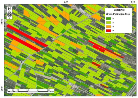
Figure 1.
Pollination risk scores at the local level. The color scale varies from green (low risk) to red (maximum risk). Qi are the i-quartiles.
Figure 2 shows the raster representation of the regional model at Comunitat Valenciana scale. Areas painted in gray represent regions where citrus production is negligible.
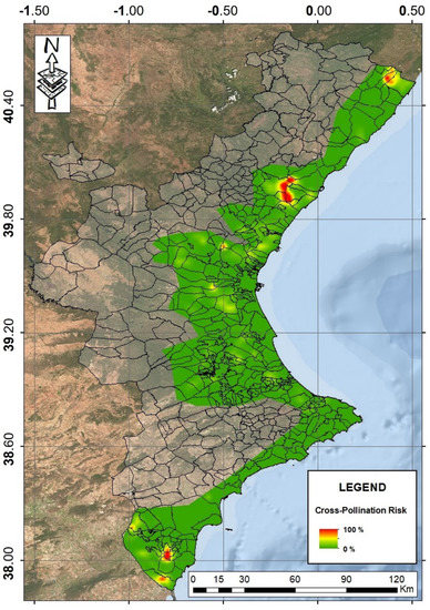
Figure 2.
Pollination risk scores at the regional level. The color scale varies from green (0 risk) to red (maximum risk, arbitrary set to 100%). Municipality boundaries are shown in black lines.
3.2. Robustness Assessment of the Local Model
Table 2 summarizes the distribution parameters of raw risk scores calculated using the reference parameters (f = 1/2.5 and Mf, = 3000 m). A very high variability of data can be observed, with a variation coefficient (standard deviation divided by mean) of 3.2. Moreover, higher values make a clearly biased distribution (the mean is more than four times larger than the median).
Table 2.
Reference risk data statistics. Max: maximum risk score. Mean: average risk score. Median: median risk score. σ: standard deviation of risk scores. CV: variation coefficient.
Table 3 describes the effect of modifying the estimated maximum flight distance of bees. As expected, the higher the distances, the higher the calculated raw risk gray level values (higher maximum and mean gray level values and higher standard deviations). Similarly, the more distinct the parameter Mf with respect to the reference, the higher the RMSE and RMSEn and the lower r. However, it can be observed that all correlation coefficients are extremely high, ranging from 0.988 to 0.999, thus revealing that relative changes due to variations in this parameter are minimal and they are almost visually negligible if we use either raw or normalized data and a linear palette to represent risk scores at the local level.
Table 3.
Effect of arbitrarily changing the Mf on risk scores. r: Pearson’s correlation coefficient with respect to reference risk scores. RMSE: root mean square error difference using raw scores. RMSEn: root mean square error difference, normalized scores (divided by Max).
A study of the effect of modifying the area factor, f, was not conducted as it is a proportional, common factor in Equation (2) and subsequently in Equation (3).
3.3. Robustness Assessment of the Reginal Model
Table 4 shows the statistics of the gray levels of the normalized image (prior to smoothing) used for the regional model. As the maximum value is around 6.8, there is at least one pixel whose value is extraordinarily high (more than six times the ratio of conventional normalization obtained by dividing by the maximum value). Furthermore, the mean is far from being close to 0.5, both facts indicating that large values are scarce, which reinforces the approach of normalizing by the 95th percentile.
Table 4.
Reference normalized image gray level statistics. Max: maximum gray level. Mean: average gray level. Median: median gray level. σ: standard deviation of gray levels. CV: variation coefficient of gray levels.
Table 5 depicts the effect of modifying the assumption of higher and lower bee flying distances. The parameters Max, Mean, and σ refer to the generated image, while SSIM is the similarity index obtained when comparing recalculated and reference images, and c, r, and l are the parameters used to calculate this similarity index.
Table 5.
Effect of modifying Mf on normalized images. Max: maximum gray level of recalculated normalized image. Mean: average gray level. Median: median gray level. σ: standard deviation. RMSE: root mean square difference with respect to the normalized reference image. c: contrast parameter in the SSIM model. r: correlation coefficient in the SSIM model. l: luminosity parameter in the SSIM model. SSIM: c ∗ r ∗ l.
As expected, the higher the differences in Mf with respect to the reference, the higher the RMSE. However, modifications of Mf strongly affect the maximum gray level in an unclear way: decreasing Mf by 1/3 (Mf = 2000) increases Max much more than increasing Mf by 1/3 (Mf = 4000). Apparently, a reduction in Mf has a greater effect on the maximum gray level than increasing Mf. On the other hand, modifications of Mf did not consistently affect the mean. The highest values of σ were obtained by decreasing its value.
Modifying the bee flying distance did not produce relevant dissimilarities between the generated and reference images, with SSIM ranging from 0.966 to 0.989. Major differences were due to contrast (c ranging from 0.985 to 0.995), while r and l were very high (ranging from 0.990 to 0.997).
Table 6 reflects the effect of modifying parameter f on raw normalized images. Negligible variations are observed when modifying it in the selected arbitrary range (0.5 to 1.29), which is equivalent to changing the raw risk by a factor in the range of 0.25 to 1.66. Again, major differences are found in maximum gray level values of the recalculated images and in contrast with respect to the reference.
Table 6.
Effect of modifying f on raw normalized images. Max: maximum gray level of recalculated normalized image. Mean: average gray level. Median: median gray level. σ: standard deviation. RMSE: root mean square difference with respect to the reference image. c: contrast parameter in the SSIM model. r: correlation coefficient in the SSIM model. l: luminosity parameter in the SSIM model. SSIM: c ∗ r ∗ l.
4. Discussion
The main reason for our work was to provide tools for helping in the solution of a long-lasting conflict of interests between citrus growers and beekeepers in Comunitat Valenciana. Our objectives were twofold: (a) to propose methods to determine cross pollination risks in Valencian citrus orchards, in order to guarantee the production of seedless fruits, and (b) to analyze the sensitivity of these models to changes in the input parameters.
We implemented two risk models for the regional and local representation of cross-pollination risks using as inputs the planted varieties, their pollinating capability, their sensitivity to pollination, the maximum flight distance of bees, the amount of sensible vegetation (by means of a factor associated to the area of the orchards), and a damping pollination function related to the distance between plots. Moreover, we analyzed the sensibility of these models to modifications in the values of the major variables. Risk scores in the context of this work are a representation of the relative assessment of actual cross-pollination risk (orchards having higher scores have higher risks).
The models presented in this study are backed by a huge sample (more than 53% of orchards of Comunitat Valencina) of actual field information from citrus orchards, which provides the results with a high degree of robustness. Our approach provides stakeholders (lawmakers, farmer unions, honey industry, cooperatives, municipalities, and so on) with geo-referenced tools for objectively determining ideal land use.
The results demonstrate that, in the case of vectorial representation of local maps, normalized scores and raw scores provide similar results if a linear scale palette is used for representation, even if Mf and f values change. They also show, in the case of raster representation of regional maps, the interest in normalizing gray levels by dividing by the 95th percentile, as such normalization maintains high correlation values and high image similarity with respect to the reference image, thus reducing the effect of changes in Mf and f values. This image similarity effect is probably caused by the risk score aggregation in 3000 × 3000 m pixels and would be further reinforced by the smoothing procedures applied to the resulting normalized image to build the final map.
The presented regional model is capable of identifying specific large areas (set of municipalities or municipality areas where the presence of bees will not pose cross-pollination risks to citrus), thus providing means for optimal hive location and management. Considering that approximately 99 mandarin-type varieties and 60 orange-type varieties are currently cultivated in our region, the proposed local model is a powerful instrument for the future planning and development of the Comunitat Valenciana varietal location distribution. Finally, our work demonstrates the interest in exploiting existing databases for generating tools for land management at different scales and assessing the actual impact of agricultural and environmental policies.
Cross-pollination can be positive for citrus cultivated in other areas in the world and for many other plant species. The geostatistical approaches presented in this work can also be applied to improve pollination when and where required. Worldwide benefits and problems related to citrus cross-pollination have been illustrated in the literature [17]. However, the presence of seeds in citrus fresh fruits as a result of cross-pollination poses serious problems to marketing in Western countries, in which consumers are accustomed to seedless fruit. This has been thoroughly addressed not only in Spain [13], but also in South Africa [18]. However, such works refer basically to the possibility of commercial varieties to induce seeds in laboratory tests. One important novelty of this work resides in the proposal of objective, data-driven geostatistical methods to assess risks in field conditions at local and regional scales.
Taking into consideration the classification of Suanno et al. [11], the models proposed in this work can be classified as observation-based, like those reported by [8,9], which differ from those denominated as process-based, like Lagrangian approaches [10] built on individual kernel functions [19] or semi-empirical models [20]. The reason for us not selecting this approach is that this last group is focused on the fate of pollen and the probability of pollination rather than on the risk assumed by a plot during its lifespan.
With respect to data used as input in these models, the large number of orchards with respect to the total citrus orchards in Comunitat Valenciana (53%) used to build the models makes it unnecessary to use interpolation techniques, like kriging, commonly used for airborne pollen forecasting [21]. According to the typology of data, the authors of [9] employed those related to pollinator nesting resources, floral resources, foraging distances, landscape configurations, and even farm management (to study the influence of agricultural practices). Contrary to our objectives, their models were aimed at predicting the relative abundance of pollinators and, subsequently the pollination services required. However, we share the idea of introducing information about the neighboring species and foraging distances in order to assess the possibility of pollination. Nevertheless, the work of [10], focused more on pollen fate, includes meteorological information, which we consider unnecessary for our work, which is focused on risks, not on probabilities.
Most of the above-mentioned literature understands the importance of conducting sensitivity analysis to determine the influence of data variations in the results. Lonsdorf et al. [8] studied the sensitivity of the model’s prediction dependence on the input variables by analyzing linear regression coefficients between different models obtained from random samples of the input parameters assumed to be uniformly distributed. Kennedy et al. [9] used different mixed models and the Akaike information criterion [22] for comparing the adequacy of the models. However, if we consider that their results are raster images, these methods basically account for relationships between pixel gray levels of different resulting images, but ignore variations in their structural information. For this reason, we preferred to use the structural similarity index that independently compares luminance (related to average gray levels) and contrast (related to standard deviations of gray levels), and not only correlation between gray levels. Alternatively, Lipsius et al. [10] studied the sensibility of their models to the quality of meteorological data by a step-by-step reduction of the information, but we consider that the input information that we use will be easily available and that testing its reduction is not necessary.
Apart from this, it must also be recognized that the small influence of variations in parameter f in the results during sensitivity analysis could be attributed to the chosen reference value. Furthermore, in relation to risk, probability can be used to figure out the chance that taking a risk will pay off, which has not been undertaken in the present work. Besides, new relevant tools can be generated from our work to (a) simulate the risk of cross-pollination that a new orchard planted with a specific variety may induce to its neighbors and (b) simulate the risk of cross-pollination that neighbors induce on new orchards, depending on the variety that will be planted. All of these issues will require further investigation.
Author Contributions
Conceptualization, E.M.; methodology, E.M., J.L.P. and C.O.; validation, E.M., J.L.P., C.O. and H.I.-S.; formal analysis, E.M.; data curation, C.O. and J.L.P.; writing—original draft preparation, E.M. and H.I.-S. All authors have read and agreed to the published version of the manuscript.
Funding
This work has been partially financed by the project “Engineering developments for the assurance of a profitable, sustainable and competitive agriculture from field to table” (internal reference number 52204) co-financed by IVIA and the European Regional Development Fund (ERDF). Héctor Izquierdo benefits of an Instituto Nacional de Investigación y Tecnología Agraria y Alimentaria (INIA) pre-doctoral contract (reference PRE2021-100395) financed by the Spanish Ministry of Science and Innovation (MCIN/AEI/10.13039/501100011033) and the European Social Fund Plus (ESF+).
Conflicts of Interest
The authors declare no conflict of interest.
References
- FAO. Citrus Fruit Statistical Compendium 2020; FAO: Rome, Italy, 2021. [Google Scholar]
- Ministerio de Agricultura, Pesca y Alimentación. Superficies y Producciones Anuales de Cultivo de Acuerdo Con el Reglamento (CE) 543/2009. Available online: https://www.mapa.gob.es/es/estadistica/temas/publicaciones/anuario-de-estadistica/2020/default.aspx?parte=3&capitulo=07&grupo=8 (accessed on 9 September 2022).
- Conselleria de Agricultura, Desarrollo Rural, Emergencia Climática y Transición Ecológica. Informe del Sector Agrario Valenciano 2020. Conselleria de Agricultura, Desarrollo Rural, Emergencia Climática y Transición Ecológica: Valencia, Spain, 2021. Available online: https://agroambient.gva.es/es/informes-del-sector-agrario-valenciano (accessed on 8 September 2022).
- Free, J.B. Insect Pollination of Crops; Academic Press: New York, NY, USA, 1970; p. 544. [Google Scholar]
- Hearn, G.H.; Watkins, W.G.; Bishop, R.K. Orange nectar and pollen in relation to bee activity. J. Econ. Entomol. 1942, 35, 321–323. [Google Scholar] [CrossRef]
- Couvillon, M.J.; Riddell Pearce, F.C.; Accleton, C.; Fensome, K.A.; Quah, S.K.; Taylor, E.; Ratnieks, F.L. Honey bee foraging distance depends on month and forage type. Apidologie 2015, 46, 61–70. [Google Scholar] [CrossRef]
- Generalitat Valenciana. Acuerdo de 18 de Marzo de 2021, del Consell, de Aprobación de Medidas para Limitar la Polinización Cruzada Entre Plantaciones de Cítricos; DOGV núm. 9047 de 24.03.2021; Generalitat Valenciana: Valencia, Spain, 2021.
- Lonsdorf, E.V.; Kremen, C.; Ricketts, T.H.; Winfree, R.; Williams, N.M.; Greenleaf, S.S. Modelling pollination services across agricultural landscapes. Ann. Bot. 2009, 103, 1589–1600. [Google Scholar] [CrossRef] [PubMed]
- Kennedy, C.M.; Lonsdorf, E.V.; Neel, M.C.; Williams, N.M.; Ricketts, T.H.; Winfree, R.; Bommarco, R.; Brittain, C.A.; Burley, A.L.; Cariveau, D.P.; et al. A global quantitative synthesis of local and landscape effects on wild bee pollinators in agroecosystems. Ecol. Lett. 2013, 16, 584–599. [Google Scholar] [CrossRef] [PubMed]
- Lipsius, K.; Wilhelm, R.; Richter, O.; Schmalstieg, K.J.; Schiemann, J. Meteorological input data requirements to predict cross-pollination of GMO Maize with Lagrangian approaches. Environ. Biosaf. Res. 2007, 5, 151–168. [Google Scholar] [CrossRef] [PubMed]
- Suanno, C.; Aloisi, I.; Fernández-González, D.; Del Duca, S. Pollen forecasting and its relevance in pollen allergen avoidance. Environ. Res. 2021, 200, 111150. [Google Scholar] [CrossRef] [PubMed]
- Wang, Z.; Bovik, A.C.; Sheikh, H.R. Image Quality Assessment: From Error Visibility to Structural Similarity. IEEE Trans. Image Process. 2004, 13, 600–612. [Google Scholar] [CrossRef] [PubMed]
- Bono, R.; Soler, J.; Villalba, D.; Salvia, J.; Bellver, R.; Mares, M.; Méndez, J.V.; Gavilá, L. Cuadro de Polinizaciones. El problema de la presencia de semillas en los frutos cítricos. Ficha Técnica. In Serie Citricultura: 5; Conselleria d’Agricultura Pesca i Alimentació, Generalitat Valenciana: Valencia, Spain, 2006. [Google Scholar]
- QGIS Development Team. QGIS Geographic Information System. Open-Source Geospatial Foundation Project. 2022. Available online: http://qgis.osgeo.org (accessed on 8 September 2022).
- Mapshaper. Available online: https://mapshaper.org/ (accessed on 8 September 2022).
- Wang, Z.; Bovik, A.C. A universal image quality index. IEEE Signal Process. Lett. 2002, 9, 81–84. [Google Scholar] [CrossRef]
- Gurung, S.; Chettri, A. Threat to Citrus in a Global Pollinator Decline Scenario: Current Understanding of Its Pollination Requirements and Future Directions. In Plant Reproductive Ecology: Recent Advances, 2nd ed.; Rustagi, A., Chaudhry, B., Eds.; IntechOpen: London, UK, 2021; p. 134. [Google Scholar]
- Barry, G.H. A Prediction Model to Determine the Cross-Pollination Ability of Citrus spp. Master’s Thesis, University of Natal, Pieteermaritzburg, South Africa, 1995. Available online: http://hdl.handle.net/10413/11772 (accessed on 1 September 2022).
- Klein, E.K.; Lavigne, C.; Picault, H.; Renard, M.; Gouyon, P.H. Pollen dispersal of oilseed rape: Estimation of the dispersal function and effects of field dimension. J. Appl. Ecol. 2005, 43, 141–151. [Google Scholar] [CrossRef]
- VDI Richtlinien, VDI 3945; VDI Standards. Environmental Meteorology-Atmospheric Dispersion Models-Particle Model. Beuth Verlag GmbH: Berlin, Germany, 2020.
- Picornell, A.; Oteros, J.; Trigo, M.M.; Gharbi, D.; Docampo Fernández, S.; Melgar Caballero, M.; Toro, F.J.; García-Sánchez, J.; Ruiz-Mata, R.; Cabezudo, B.; et al. Increasing resolution of airborne pollen forecasting at a discrete sampled area in the southwest Mediterranean Basin. Chemosphere 2019, 234, 668–681. [Google Scholar] [CrossRef] [PubMed]
- Akaike, H. Information Theory and an Extension of the Maximum Likelihood Principle. In Proceedings of the Second International Symposium on Information Theory, Tsahkadsor, Armenia, USSR, 2–8 September 1971; Petrov, B.N., Caski, F., Eds.; Akademiai Kiado: Budapest, Hungary, 1973; pp. 267–281. [Google Scholar]


Publisher’s Note: MDPI stays neutral with regard to jurisdictional claims in published maps and institutional affiliations. |
© 2022 by the authors. Licensee MDPI, Basel, Switzerland. This article is an open access article distributed under the terms and conditions of the Creative Commons Attribution (CC BY) license (https://creativecommons.org/licenses/by/4.0/).